


1. Introduction
The detection and characterization of human activity-induced small-scale seismic disturbances in the subsurface (“microseismic”) is of great importance in the natural resources sector. Specifically in oil and gas production, microseismic monitoring helps managing reservoirs for recovery optimization, and with hazard management (Nederlandse Aardolie Maatschappij (NAM), Grechka and Heigl, Reference Grechka and Heigl2017). Most applications today are related to mapping the progress of hydraulic fracturing operations in shale reservoirs. In this paper, we outline a new approach for simultaneously detecting and characterizing multiple microseismic events directly from long passive seismic recordings. In particular, we illustrate the approach using a large 3D marine heterogeneous velocity model composed of a few million voxels with pre-specified density, compressional (P-wave), and shear (S-wave) sound velocities. We then take a Bayesian inference route and obtain samples from the multimodal posterior distribution for multiple superimposed microseismic events in the joint space, time, and amplitude domain. Conventional geophysical approaches use (usually picked or windowed) signal travel-times in various inversion schemes (Grechka and Heigl, Reference Grechka and Heigl2017), homogenous models (Eisner et al., Reference Eisner, Duncan, Heigl and Keller2009), or wavefield migration (Rentsch et al., Reference Rentsch, Buske, Lüth and Shapiro2006) which are used for locating hypocenters and some event or for simultaneously deriving subsurface structures and the velocity model, that is, “tomography,” “imaging” (Zhang et al., Reference Zhang, Sarkar, Toksӧz, Kuleli and Al-Kindy2009). Almost all of these approaches have in common that they are not fully automated, cannot use very long seismic recordings with multiple events, have difficulty with complex heterogeneous 3D velocity models, and/or are impractically sensitive to noise.
In this study, we focus on event location and characterization assuming that an accurate 3D heterogeneous velocity model is available. This is however not a fundamental constraint of our approach since the inversion could be extended to the velocity model itself to perform imaging and tomography tasks. To demonstrate the workings of our method, we use a marine velocity model with receivers on the seabed at a depth of z = 244 voxels. We then perform 4,000 independent simulations of forward wave propagation from random spatial event locations with unit (1 MPa explosive source) amplitude, using an elastic wave equation solver on GPUs, as described in Das et al. (Reference Das, Chen and Hobson2017) and record the seismograms on 23 surface receivers. More details on the source wavelet type, type of measurements and other details of forward simulations are given in Das et al. (Reference Das, Chen and Hobson2017), but here we mainly focus on the datasets for the pressure measurements given by the hydrophones. We then apply a time-domain compression to create a smooth mapping between the event locations and the compressed components of the seismograms. The training and testing of this mapping make use of an ensemble of Gaussian process (GP) regression models using the automatic relevance discovery (ARD) Matérn 3/2 kernel and linear basis function. This trained ensemble of GP model is referred as the proxy or surrogate meta-model hereafter and has been detailed in Das et al. (Reference Das, Chen, Hobson, Phadke, van Beest, Goudswaard and Hohl2018). Making use of this trained fast proxy-based forward model as a means for multi-receiver seismogram generation from random microseismic events, the events’ spatial location estimation from given noisy seismograms can be seen as a 3D spatial inference problem using an optimizer or Bayesian sampler with a suitable choice of objective function or likelihood (Tarantola, Reference Tarantola2005). However, apart from the spatial locations, the events’ amplitudes and origin times are also of interest, and can be simulated with linear scaling and translation operations on unit amplitude seismic responses at random locations, and then combined together for multiple superimposed events as detailed in Das et al. (Reference Das, Chen and Hobson2017). There have been few previous attempts of uncertainty quantification in microseismic location inversion (Eisner et al., Reference Eisner, Duncan, Heigl and Keller2009; Xuan and Sava, Reference Xuan and Sava2010) via Bayesian methods, mostly using P/S-wave arrival time picking (Massin and Malcolm, Reference Massin and Malcolm2018) for simultaneous estimation of an uncertain velocity model (Zhang et al., Reference Zhang, Rector and Nava2017), estimation of joint and relative microseismic locations (Poliannikov et al., Reference Poliannikov, Prange, Malcolm and Djikpesse2013, Reference Poliannikov, Prange, Malcolm and Djikpesse2014) or even moment tensor estimation (Pugh and White, Reference Pugh and White2018), etc. However, full multi-receiver seismic data-based inference has its own merits over arrival time picking and is suitable for jointly estimating event amplitudes and origin times along with the locations. Also given noisy seismograms, finding multiple superimposed events requires a multimodal Bayesian inference in the 5D spatio-temporal-amplitude domain. Not all the events will make the same contribution to the recorded seismic data and consequently, near-surface (shallow) or higher-amplitude events become more prominent in the multimodal posterior inference as compared to the lower-amplitude deep sources. Detectable multiple true events will still appear as distinct peaks in the likelihood surface while we scan with a single event model which allows a significantly low-dimensional search as discussed in (Hobson and McLachlan, Reference Hobson and McLachlan2003; Hobson et al., Reference Hobson, Rocha and Savage2009; Feroz et al., Reference Feroz, Balan and Hobson2011). This paper aims to give a brief overview of the methodology using the MultiNest algorithm (Feroz and Hobson, Reference Feroz and Hobson2008; Feroz et al., Reference Feroz, Hobson and Bridges2009) to simultaneously detect multiple microseismic events in the subsurface. We also show the associated likelihood landscapes and how to use clustering to detect mode-separated events.
2. Bayesian Inference
In Bayesian parameter and uncertainty estimation, the posterior distribution  $ P\left(\theta \right) $ gives the complete inference for the parameters of interest $ \theta $. The posterior can be expressed in a probabilistic notation or as the product of the likelihood function $ L\left(\theta \right) $ and the prior $ \tilde{\pi}\left(\theta \right) $, normalized by the Bayesian evidence for observed data D and hypothesis H:
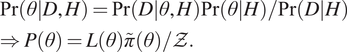 $$ {\displaystyle \begin{array}{l}\Pr \left(\left.\theta \right|D,H\right)=\Pr \left(\left.D\right|\theta, H\right)\Pr \left(\left.\theta \right|H\right)/\Pr \left(\left.D\right|H\right)\\ {}\Rightarrow P\left(\theta \right)=L\left(\theta \right)\tilde{\pi}\left(\theta \right)/\mathcal{Z}.\end{array}} $$
 The denominator of (1) is known as the marginal likelihood or Bayesian evidence ( $ \mathcal{Z} $):
 $$ \mathcal{Z}=\Pr \left(\left.D\right|H\right)=\int L\left(\theta \right)\tilde{\pi}\left(\theta \right) d\theta, $$
and not only normalizes the posterior distribution of model parameters (conditional to the data) but also plays a key role in model selection using the Bayes factor or posterior odds-ratio.
Calculating the evidence using standard Markov Chain Monte Carlo (MCMC) methods and simultaneously navigating a multimodal posterior distribution is a challenging task (Skilling, Reference Skilling2006; Shaw et al., Reference Shaw, Bridges and Hobson2007; Feroz and Hobson, Reference Feroz and Hobson2008). Improved algorithms like multimodal nested sampling have emerged to generate samples from posterior distribution with multiple modes and/or with wide curving degeneracies. This has been shown to outperform most MCMC variants for simultaneous detection of multiple objects in (Feroz and Hobson, Reference Feroz and Hobson2008; Feroz et al., Reference Feroz, Hobson and Bridges2009). We here employ the MultiNest algorithm for 5D spatio-temporal-amplitude inference of multiple microseismic events, since the posterior shows both multi-modal nature and thin curving degeneracies in different combinations of the parameters of interest which is described in the following sections.
3. Microseismic Event Detection Workflow
Figure 1 shows the schematic diagram for the multiple microseismic event detection workflow using Bayesian inference with multimodal nested sampling. Starting from the 3D heterogeneous marine velocity model, we generate the seismograms at the receivers placed at the sea-bed, using an elastic wave propagation solver on Tesla K20 GPUs (Das et al., Reference Das, Chen and Hobson2017). Next, the time domain compressed seismic signals are fed to a machine learning algorithm, that is, an ensemble of GP surrogate models for each compressed component using the ARD Matérn 3/2 kernel with linear basis. The learnt surrogate meta-model then undergoes testing on independent held out datasets as detailed in Das et al. (Reference Das, Chen, Hobson, Phadke, van Beest, Goudswaard and Hohl2018), to verify the high accuracy of the proxy generated seismograms to be used in the inference process. We fuse all the 23 receivers’ data in a Gaussian likelihood function (3) as:
 $$ L\left(\theta \right)=\Pr \left(\left.D\right|\theta, H\right)=\frac{1}{\sqrt{{\left(2\pi \right)}^N\left|C\right|}}\exp \left[-\frac{1}{2}{\left(Y-\hat{Y}\right)}^T{C}^{-1}\left(Y-\hat{Y}\right)\right], $$
Figure 1. Schematic diagram of the basic steps of Bayesian microseismic event detection workflow.
since this yields a better detection accuracy as compared to selecting only a subset of them, albeit at the cost of increased computational burden.
Here  $ \left\{Y,\hat{Y}\right\} $ represent the measured noisy and noiseless proxy generated template seismograms, N is the dimension of the multi-receiver data reshaped as a 1D array and C is the covariance matrix of the noise on the data and can be calculated as (4), which is assumed to be diagonal for simplicity and given as:
 $$ C=\unicode{x1D53C}\left[{\left(Y-\overline{Y}\right)}^T\left(Y-\overline{Y}\right)\right]={\sigma}^2I, $$
 where  $ \unicode{x1D53C}\left[\cdot \right] $ represents the expectation operator and the additive noise $ \sigma $ is in Pascal.
We create synthetic seismograms (Y) using (5), by superimposing, for demonstration, Ne = 3 events at random locations with different amplitudes (Ao) and having equally spaced origin times (To = 250)
 $$ {\displaystyle \begin{array}{l}{Y}_{template}=f\left({x}_o,\hskip.3em {y}_o,\hskip.3em {z}_o\right),\\ {}Y=\sum \limits_{n=1}^{Ne}{A}_o^n{Y}_{template}\left({x}_o^n,,,\hskip.3em ,{y}_o^n,,,\hskip.3em ,{z}_o^n,,,\hskip.3em ,t-{T}_o^n\right)+\mathcal{N}\left(0,{\sigma}^2\right).\end{array}} $$
 For the microseismic events with different amplitudes, the explosive source strengths are randomly chosen between  $ {A}_o\in \left[0,80\right] $ MPa, that is,
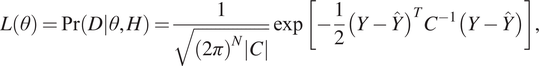
  $ {A}_1=68,{A}_2=32,{A}_3=52 $, where the second event has relatively low amplitude as compared to the other two. Representative simulated seismograms on the 23 receivers are shown in Figure 2. Due to having different depth (z), the arrival times (Ta) are not equally spaced on the superimposed seismograms in Figure 2, although the origin times are equally spaced, since responses of deeper events take more time to reach the surface receivers. The synthetic seismic data have been corrupted with additive white Gaussian noise of standard deviation (std) σ = 3 × 10⁴ Pa. The corresponding signal to noise ratios (SNRs) are also calculated as the ratio of the root mean squared energy of the signal to the noise and take a negative value here in decibel (dB) scale, indicating a highly noisy background. This creates synthetic noisy seismic traces on 23 receivers each of which is 6 s long and having three events where the temporal resolution is 4 ms, thus having total 1,500-time samples in the episode to be scanned. Regarding these synthetic noisy seismic traces as the “observed data,” and then assuming the noise standard deviation to be known beforehand (which can also be estimated using a previously collected field-data), we then use the proxy-generated seismograms to compare with the observed data and construct the likelihood function. The presence of multiple events in the seismic traces leads to a multimodal likelihood function to identify the modes separately for the event detection as described in Hobson and McLachlan (Reference Hobson and McLachlan2003), Hobson et al. (Reference Hobson, Rocha and Savage2009), Feroz and Hobson (Reference Feroz and Hobson2008).
Figure 2. Noiseless and noisy seismograms generated with three superimposed microseismic events with different origin times and different amplitudes. Noise is considered to be Gaussian with strength σ = 3 × 10⁴ Pa, giving the negative SNR (in dB) indicated in the title.
A uniform prior search range of  $ \tilde{\pi}\left(\theta \right)=x\in \mathcal{U}\left[1,81\right],\hskip.5em y\in \mathcal{U}\left[1,81\right],\hskip.5em z\in \mathcal{U}\left[1,243\right], $ $ {A}_o\in \mathcal{U}\left[0,80\right],\hskip.5em {T}_o\in \mathcal{U}\left[1,1500\right] $ has been considered in the nested sampling. Here the spatial parameters represent the voxel number of the velocity model, the source amplitude is in MPa and the origin times are discrete sample numbers in the time series data. The nested sampling algorithm will generate samples from the multimodal posterior distribution which are then marginalized for visualization. The posterior samples also allow one to obtain the maximum a-posteriori (MAP) estimate of the event parameters and the calculated Bayesian evidence enables to carry out hypothesis testing or Bayesian model selection for discriminating true vs. false events. However, using the generated samples from the MultiNest sampler, the calculated posterior distribution may have complicated shape and does not necessarily always appear as distinct peaks in the likelihood surface as functions of the event parameter pairs. As a result, the X-means or k-means clustering algorithms (which is the default option) for mode separation in MultiNest algorithm (Feroz et al., Reference Feroz, Hobson and Bridges2009) might split long thin clusters into many smaller ellipsoidal clusters, indicating many possible events. Therefore, we instead use the density-based spatial clustering of applications with noise (DBSCAN) algorithm to recluster the MultiNest generated samples to identify dense cluster of points indicating possible events. In the MultiNest algorithm, there was a built in X-means or improved k-means algorithm for mode separation which looks for ellipsoidal clusters during the sampling process and shrinking the prior volume. The main idea here is to generate samples from the multimodal likelihood function and then apply a suitable clustering method based on the patterns of the sampled data points.
We here apply the DBSCAN clustering on the two parameters—depth vs. origin time (Z-To) only because these two parameter pairs clearly show separated long dense regions of sampled points for each event. We set the two controlling parameters of DBSCAN namely maximum distance in the same neighborhood ε = 20 and the minimum number of points per cluster minPts = 35, to allow clustering on long curving degeneracies as a continuous and dense cluster of sampled points. Unlike the other clustering methods, the DBSCAN does not need to specify the number of clusters and can automatically find dense cluster of points with arbitrary shape while labeling points far away from the dense clusters as noise. More details on DBSCAN clustering can be found in Kriegel et al. (Reference Kriegel, Krӧger, Sander and Zimek2011) and Schubert et al. (Reference Schubert, Sander, Ester, Kriegel and Xu2017).
4. 5D Spatio-Temporal-Amplitude Inference for Detecting Multiple Microseismic Events
The details of multiple event detection using Bayesian nested sampling have been previously discussed in Hobson and McLachlan (Reference Hobson and McLachlan2003) and Hobson et al. (Reference Hobson, Rocha and Savage2009). The main idea here is to start from a few randomly sampled live points (N live) within the prior volume. New samples are then generated in subsequent iterations as the prior volume shrinks toward the high-likelihood regions. This locates prominent peaks at different places in the posterior distribution corresponding to multiple objects (here microseismic events). Previously, it has been shown that if the contribution of different objects to the superimposed data is reasonably well separated, this approach of using multimodal nested sampling can allow multiple event detection as well as posterior inference around each detected mode (Feroz et al., Reference Feroz, Balan and Hobson2011). This also helps in avoiding searching a high dimensional and often trans-dimensional parameter space for varying (or unknown) number of objects and their associated parameters. Here, the fast Bayesian sampler MultiNest algorithm implemented in Fortran is called through a Python wrapper so as to facilitate communication with the Matlab based trained proxy meta-model in each iteration via the Matlab engine API for Python (MATLAB API for Python).
In the context of accurate profile likelihood exploration with many small hidden structures, usually a scan with high N live is required as also suggested in Feroz et al. (Reference Feroz, Cranmer, Hobson, de Austri and Trotta2011). Here we report the scanning results using N live = {300, 500}, where the latter case massively increases the total number of likelihood calls (N like) which gets almost doubled as reported in Table 1, along with the calculated evidence and the associated errors. The null hypothesis H 0 in Table 1 yields deterministic result due to not having any event parameter to search on. Therefore, it does not give error bounds on the log-evidence. The sampling efficiency in the MultiNest sampler is set to 0.3 which is reasonable for both parameter estimation and evidence calculation. After the samples are generated from MultiNest sampler, they are fed to the DBSCAN clustering algorithm to find dense regions in the depth vs. origin time (Z vs. To) scatterplots. This is shown in the 2D scatterplots of the event parameter pairs in Figure 3 where the points are colored for different events otherwise labeled as noise. In Figure 3, the ground truth parameters of the three events are shown as blue-stars to indicate that the sampled points are likely to get clustered near the high-likelihood regions or the ground truth. It is interesting to note that the likelihood draws are not equal for all microseismic events depending on the depth and the strength of the sources which is especially prominent in the depth vs. origin time (Z vs. To) scatterplots where the thin degenerated likelihood surfaces are prominent for each microseismic source. Similar low-resolution scanning results with N live = 300 are shown in the supplementary material for brevity. We note that the two stronger events on the seismic data are accurately identified by the multimodal sampling process followed by the clustering algorithm, even in a highly noisy background, whereas for the low amplitude event, the uncertainty is larger. For the 2D sampled points in Figure 3, we observe three almost parallel thin curving degeneracies in the origin time vs. depth scatterplots, indicating the fact that an earlier deep event may often be confused with a recent shallow source. As evident from the sampled points, the original time and depth detection results are correlated and as such the high-density region forms a thin line rather than a narrow region in the 5D space. Here, the microseismic sources are characterized in the joint spatio-temporal-amplitude domain with mode separation and can be better isolated as compared to the existing methods of microseismic event detection based on seismic migration or travel-time inversion techniques. However, with high-resolution scan or large N live, although the sampled likelihood points easily latch on to the peaks at the true event parameters, this can become computationally demanding and sometimes may find many spurious clusters in the low-likelihood regions. These can be filtered out using a local evidence-based criterion which may be explored in future by merging the DBSCAN inside MultiNest sampling during the cluster formation and for local evidence calculation. By using the DBSCAN clustering method, we do not need to specify the number of clusters as it automatically finds the high-density regions and the samples from the low-density regions are identified as noise which can be seen in Figure 3. Therefore, we do not need to explicitly teach the unsupervised learning algorithm how many clusters or events are present in the data, although the number of events is apparent from the visual inspection of the number of thin parallel lines in the Z vs. To plots in Figure 3. Another fourth event at the same location and origin time, that is, occurrence of multiple events with same parameters would be merged with one of the previously detected events with a higher amplitude, so will not be modeled as a separate event.
Table 1. Bayesian inference results for event detection with different amplitudes, variations in the number of likelihood calls with N live, and the calculated evidence with error.
Abbreviation: SNR, signal to noise ratio.

Figure 3. Points sampled by the MultiNest algorithm for three microseismic events with different amplitudes which are then clustered using the DBSCAN algorithm. Pairwise scatter plots are shown for the five parameters of microseismic events while scanning with different resolution parameter (a) N live = 500 (high), (b) N live = 300 (low). The three events are identified as distinct clusters (indicated as red, green, and magenta dots) along with noise (black dots). The low amplitude source is less prominent as compared to the higher amplitude events. The blue-stars represent the true parameters of the microseismic events.
For the same noisy seismic data shown in Figure 2, we first aim to test the null hypothesis (H 0) that there is no event in the seismogram (by setting the amplitude parameter as zero in the model) against the alternative hypothesis (H 1) that it has at least one event (with a template for single microseismic event) in the episode. It is seen from the difference in the Bayesian evidences for the two cases in Table 1 that for this synthetic noisy seismic data, the alternative hypothesis is strongly favored as per the Jeffrey’s scale and can be represented by the posterior odd ratio (Feroz et al., Reference Feroz, Balan and Hobson2011) as:
 $$ {\displaystyle \begin{array}{l}\mathcal{P}=\log (R)=\log \left[\frac{P\left(\left.{H}_1\right|D\right)}{P\left(\left.{H}_0\right|D\right)}\right]=\log \left[\frac{P\left(\left.D\right|{H}_1\right)}{P\left(\left.D\right|{H}_0\right)}\cdot \frac{P\left({H}_1\right)}{P\left({H}_0\right)}\right]=\log \left[\frac{{\mathcal{Z}}_{H_1}^D}{{\mathcal{Z}}_{H_0}^D}\cdot \frac{P\left({H}_1\right)}{P\left({H}_0\right)}\right]=\log \left[\frac{{\mathcal{Z}}_{H_1}^D}{{\mathcal{Z}}_{H_0}^D}\right]\\ {}\hskip1em =\log \left[{\mathcal{Z}}_{H_1}^D\right]-\log \left[{\mathcal{Z}}_{H_0}^D\right]=4168.5.\end{array}} $$
It is evident from Figure 3 that there are three detected events in the Z vs. To scatterplot, given by the DBSCAN clustering of the MultiNest generated samples. However, due to higher contribution of Event 1 and Event 3 on the seismic trace, the sampler spends less time on the weak low amplitude Event 2 rather than the stronger ones. This has been discussed in the context of unequal and overlapping modes in Feroz et al. (Reference Feroz, Balan and Hobson2011). To extend the methodology, one should ensure the seismic traces do not have too many events by running the algorithm on a smaller sliding time-window fashion instead, since the large influence of strong events are likely to supersede simultaneous detection of weak events. However, from the results in Figure 3, the three clusters of points are clearly identified for three microseismic events, although the uncertainties around them might be different if the event amplitudes vary widely.
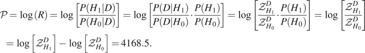
Next, we show the marginalized posterior distributions using the DBSCAN clustering and then resampling the mode separated samples, which are shown in Figure 4 as corner plots for the three different amplitude events, respectively. The diagonals of the corner plots represent the 1D marginalized posterior distributions which easily give the peaks as the MAP estimates of the parameters of interest. The lower triangular parts, below the diagonals show the pairwise 2D kernel density estimate (KDE) of the posterior contours which are mostly sparse in Figure 4a,c, due to large concentration of points in a narrow region. The upper triangular parts show the pairwise scatterplots which are colored using the log-likelihood values at each point. As discussed before for Event 1 and Event 3 in Figure 4a,c, the spatial locations and origin time can be accurately detected, although the event amplitude parameters have larger uncertainty. For Event 2 in Figure 4b, a thin chain of points can be observed in the depth vs. origin time (Z vs. To) domain and this detection has higher uncertainty due to low amplitude of this event, as compared to the rest cases, which may be often confused with background noise by the traditional methods of microseismic event detection. Due to having a large tail of the mode separated posterior plots for all the three events, we have concentrated the scatter, 2D KDE and 1D marginal plots in Figure 4 near the mode of the posterior distributions by narrowing the plotting ranges around 0.1–0.9 quantile of the clustered data for each event. Although the mode separated posterior plots yield more uncertainty for the weak event as shown in Figure 4b, it generates parallel lines for each event in the Z vs. To plot in Figure 3. Our mode separation clustering results are found to be robust as shown in Figure 3 on the Z vs. To domain where it shows three parallel curving degeneracies indicating the presence of three microseismic events in spite of having high-background noise. Since the amplitude of the green cluster for Event 2 is relatively low, this gets manifested as higher uncertainty for Event 2. But the clustering algorithm still indicates the presence of three microseismic events which has been explored next to test the robustness of the DBSCAN clustering algorithm. We have shown the scan with two different live point or resolution parameter settings (N live = 300, 500) which show similar patterns with different resolution of the inference. Mode separated posterior plots for the low-resolution scan with N live = 300 are provided in the supplementary material for brevity.
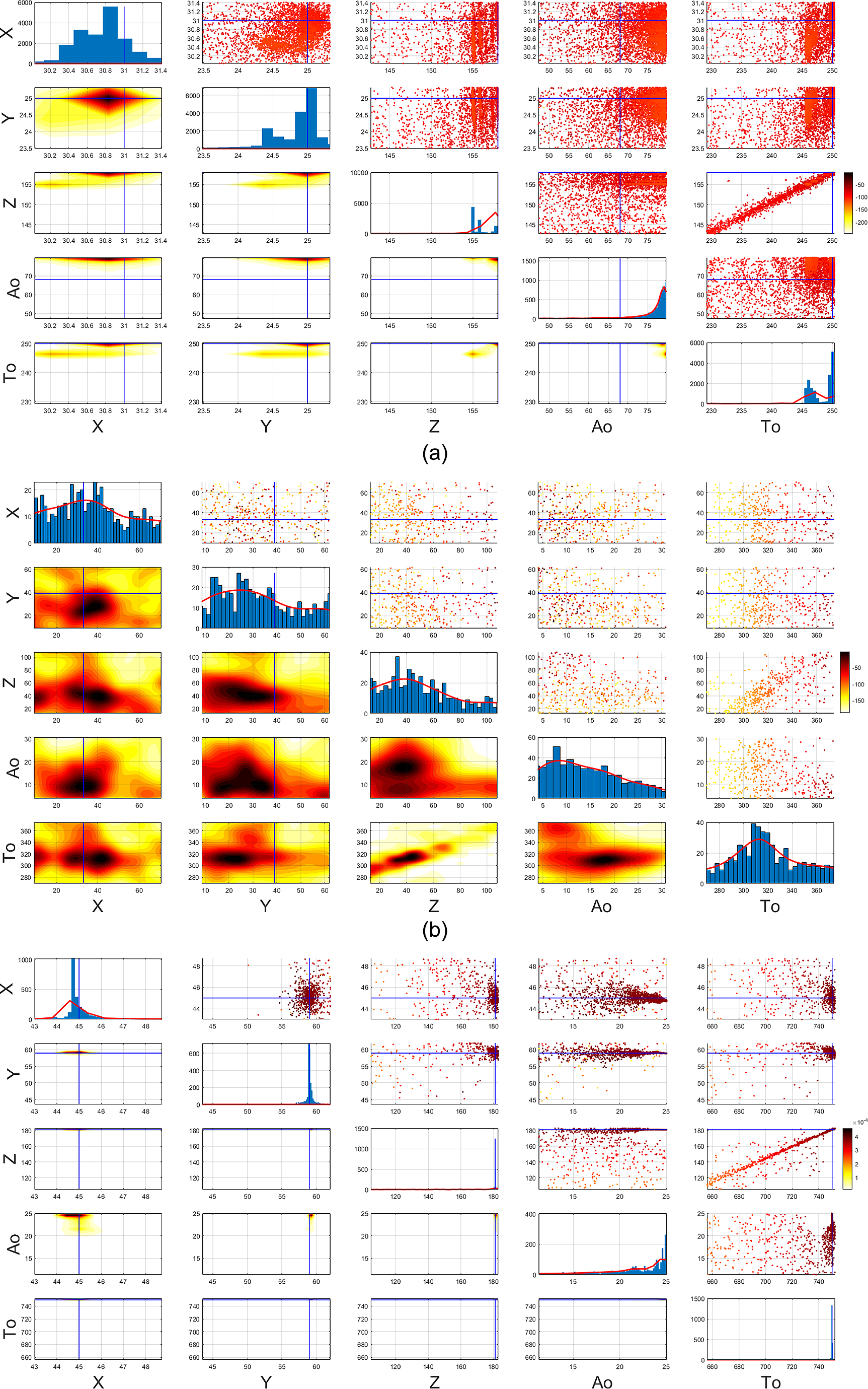
Figure 4. Mode separated posterior distribution with N live = 500 for microseismic events with (a) Event 1, (b) Event 2, and (c) Event 3. The blue lines show the true parameters of the events. Event 1 and Event 3 are strongly detected because of their high amplitude, while Event 2 is weakly detected with more uncertainty due to its relatively low amplitude. Color bar represents the likelihood of each sampled point.
Also, depending on the number of samples present in each cluster, the local evidence can be calculated which shows the cluster with more samples indicating a strong detection. Whereas other weak events where the height of the likelihood function is shorter, does gather samples proportional to its contribution toward the likelihood function. Therefore, it is important to separate out the strong and weak detections and then generate posterior density plots for each of these modes representing separate microseismic events. Since the MultiNest’s default mode separation would expect ellipsoidal shaped clusters due to the built-in X-means clustering, it would separate the thin curving degeneracies into multiple smaller clusters, calculating many local evidence values, per spurious cluster. Therefore, we adopt a post-hoc approach to recluster all the sampled datapoints visited by the MultiNest sampler, using the DBSCAN algorithm and rely on the global evidence for confirmatory hypothesis testing.
In Figure 4 the number of samples vary widely for each detected event since the contribution of all the modes toward the combined likelihood is not equal due to the difference in their amplitudes. The MultiNest sampler quickly latches on to the strongest mode and draws more samples from there, while it also samples other weaker modes of the likelihood surface. The SNR has been calculated on the whole superimposed signal comprising of the three events shown in the seismogram in Figure 2 and not the individual microseismic events. For detection of weaker sources/events, it may be difficult for a high-noise level. However, while fusing the seismic data from 23 receivers, we observe a reliable detection performance, which may not be possible to detect using fewer receivers’ data, since the likelihood will be fatter in the latter case. This shows the superiority of the proposed Bayesian microseismic event detection method over the existing non-Bayesian approaches, as discussed before.
Next in Figure 5 we show the effect of perturbing the used hyperparameters of the DBSCAN clustering algorithm for both the high- and low-resolution scan with different N live. We consider the first three strongest detections with highest number of points as true microseismic event detection and then consider rest of the samples as noise. Figure 5a for the high-resolution scan shows that within the range of DBSCAN hyperparameters  $ \varepsilon \in \left[16,20\right],\hskip0.5em \mathrm{minPts}\in \left[34,38\right] $, we reliably get three clusters as the three parallel lines are efficiently identified as thin continuous clusters. However, the uncertainty or the tail of Event 3 in Figure 5a is larger with $ \varepsilon =20 $. It is important to mention that the choice of the mode separation using the DBSCAN clustering instead of default X-means algorithm embedded in the MultiNest sampler is not guided by any prior knowledge of the number of microseismic events. The three parallel curves in the Z-To plot show there may be three possible events which do not come from the prior knowledge but emerges from the data analysis itself. This guides us to choose the DBSCAN parameters, within a range that yields three clusters and effectively separates the modes/clusters. Also, the choice of the DBSCAN hyperparameter is not informed from the prior knowledge of the number of events or true parameters of the events but it appears from the inspection of the Z-To scatter plots in Figure 3 which shows three thin parallel curves. The range of DBSCAN parameters are mentioned in the caption of Figure 5 that yields three clusters for all the sampled points for high-resolution scanning. Since the DBSCAN clustering may be sensitive to the selection of its hyperparameters, we have shown their variations which may guide us to select them for identifying the right number of clusters and also to investigate how much noise we allow to go into the clusters.
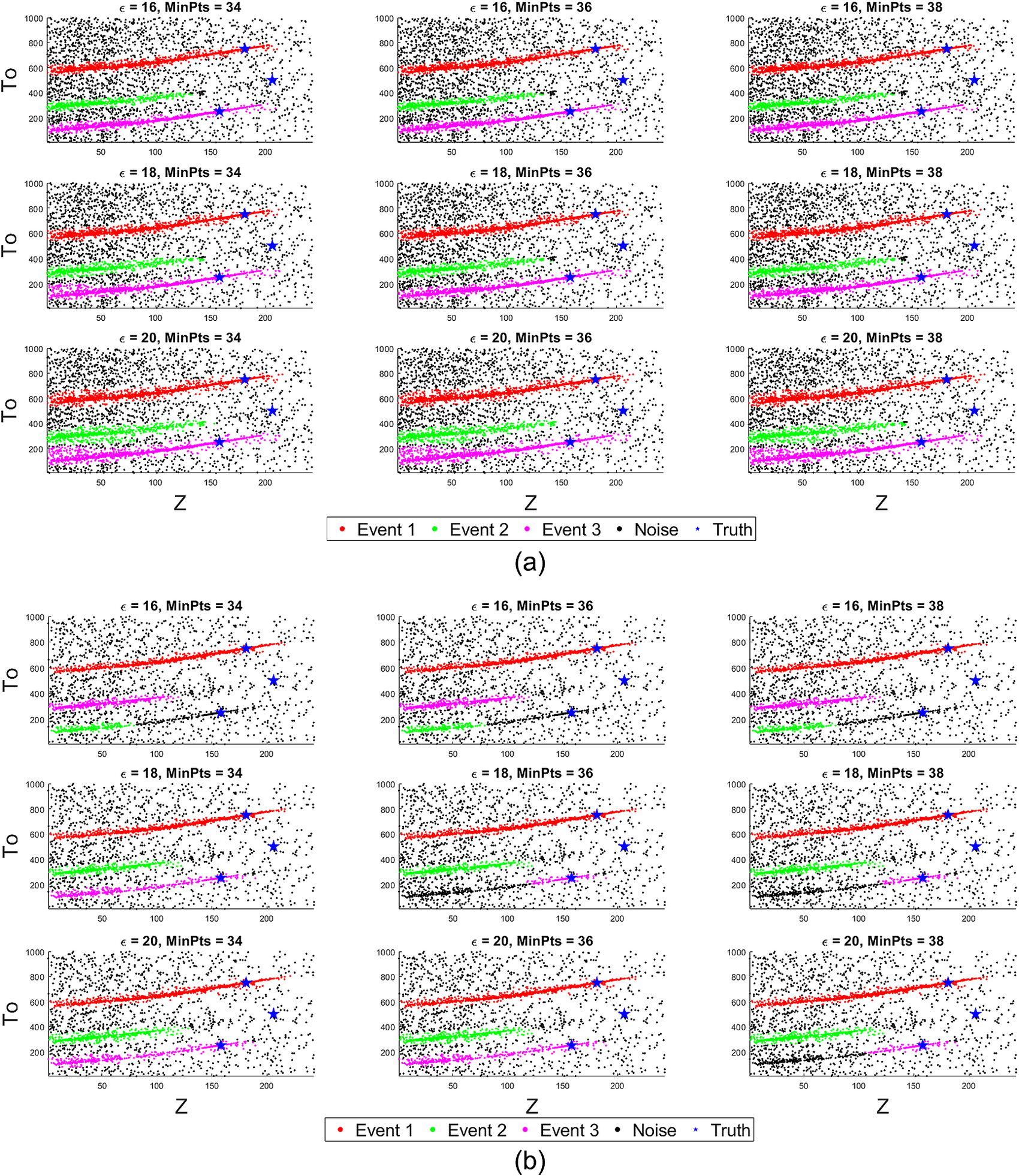
Figure 5. Robustness of the DBSCAN clustering algorithm for identifying the number of events, while discriminating against noisy samples. DBSCAN hyperparameter range  $ \varepsilon \in \left[16,20\right],\mathrm{minPts}\in \left[34,38\right] $ is found to be the most robust interval which consistently yields three clusters for the high-resolution scanning with N live = 500 (in subplot a). Outside these range of hyperparameters many small clusters are generated. The low-resolution scanning with N live = 300 (in subplot b) shows even narrower range $ \left(\varepsilon =18,\mathrm{minPts}=34\right),\hskip0.5em \left(\varepsilon =20,\mathrm{minPts}=34\right),\hskip0.5em \left(\varepsilon =20,\mathrm{minPts}=36\right) $ where the three clusters are found.
However, the DBSCAN clustering result is not very robust for scanning with a low-resolution parameter N live = 300 since it yields a smaller number of sampled points and there is lack of continuity in the thin degenerated clusters, especially for Event 3. It is evident from Figure 5b that with the three cases  $ \left(\varepsilon =18,\mathrm{minPts}=34\right),\hskip0.5em \left(\varepsilon =20,\mathrm{minPts}=34\right),\hskip0.5em \left(\varepsilon =20,\mathrm{minPts}=36\right) $, we reliably get three clusters. However, in other cases, the Cluster 3 is broken into two separate clusters due to the broken region of the gathered samples for Event 3 which shows the importance of high-resolution scanning (N live) in MultiNest, although it increases the overall computational budget. For wider variation for the low-resolution scan with N live = 300, the DBSCAN algorithm detects a larger number of clusters where the strongest three are colored and considered to be true while the rest of the weak clusters are merged with the background noise in Figure 5b. Previous works mentioned that the choice of the DBSCAN hyperparameters depends largely on the data-specific domain knowledge and it has been shown to work reliably well for 1–30% added noise (Schubert et al., Reference Schubert, Sander, Ester, Kriegel and Xu2017) but in the present scenario the added noise is much higher. A too high value for minPts would merge multiple clusters into one and add too much noise into the mode separated clusters. Also a relatively low value of ε is preferred that will allow to explore thin curving degeneracies as found in this study. Although there have been few studies on automatic selection of DBSCAN hyperparameters based on meta-heuristic optimization (Karami and Johansson, Reference Karami and Johansson2014) and several of its modified versions (Khan et al., Reference Khan, Rehman, Aziz, Fong and Sarasvady2014), a detailed parametric study of the hyperparameters as a function of MultiNest resolution parameter (N live) and noise in the seismic data (σ) are beyond the scope of the current work and may be investigated in the future.
5. Discussions
In order to ensure the identifiability of the events, we have used the sorted uniform prior distribution to draw samples which helps us in identifying the events in the correct order. However, ordering of the events is not a major concern here since the idea is to visualize each detected event separately as a posterior distribution in the 5D event parameter space rather than focussing on what order they occur in origin time, amplitude, and spatial co-ordinates. Although the Bayesian sampling is carried out in the 5D multimodal likelihood surface, but the generated samples are then clustered in the origin time vs. depth domain since the separation of the events best appears in this reduced 2D domain although the inference is done in the original 5D space. Moreover, we observe that there is more uncertainty on the amplitude parameter as compared to the spatial location and origin time parameters. In Figure 4, the 2D KDE plots of the mode separated posteriors use a Gaussian kernel. However, due to high concentration of samples at a single location, the distribution tends toward a super-Gaussian which appears as a tiny region in the 2D KDE surface plots. However, in the scatter plots on the upper triangular part one can clearly identify the concentration of samples near the ground truth as compared to the 2D KDE plots.
Regarding the main achievements of this paper, the seismological model and the likelihood function are developed in our earlier work (Das et al., Reference Das, Chen, Hobson, Phadke, van Beest, Goudswaard and Hohl2018) using a frequentist or maximum likelihood treatment for the unimodal event detection problem and also the MultiNest sampler has been previously described in Feroz and Hobson (Reference Feroz and Hobson2008) and Feroz et al. (Reference Feroz, Hobson and Bridges2009). On contrary, this paper uses a full Bayesian approach for sampling using a multimodal likelihood function as well as shows the mode separation of the samples drawn from multimodal likelihood function with high multicollinearity or multiple thin curving degeneracies. Therefore, the current work significantly advances this challenging seismological and geotechnical engineering problem over the state-of-the-art methods of microseismic event detection, with parameter estimation, uncertainty quantification, evidence-based hypothesis testing of finding at least one event, and mode separated posterior visualization.
We also found that the DBSCAN clustering on the 5D sampled points does not always yield a robust number of clusters on this data outside the recommended range of hyperparameters  $ \varepsilon \in \left[16,20\right],\mathrm{minPts}\in \left[34,38\right] $. There could be a separate study on choosing optimal parameters of DBSCAN for different microseismic datasets which is beyond the scope of the current work. However, as a simpler approach, the 2D DBSCAN clustering within the recommended hyperparameter range yields reliable result on the Z vs. To domain. Extending the clustering on 5D space and in the presence of even more events or higher noise may need investigation of other advanced clustering algorithms which may be investigated in a future work. Also, the high concentration of points as thin clusters is evident in the scatter plots in Figure 3 on the Z vs. To domain which could easily be modeled with Euclidean distance. But, more complex posterior shapes may arise for complex source mechanisms of the microseismic events which may need an investigation of spectral clustering or similar methods which are harder to model using standard notion of distance measures.
Moreover, regarding the interpretation of the posterior plots in Figure 4, we acknowledge that separating each mode and visualizing them separately are not actually represent the true posterior in a theoretical sense but are still valuable to show high- and low-density regions for each detected event separately. This is an important aspect since a superimposed posterior plot will only show the strongest and most prominent event and will suppress the information of the weak events due to highly skewed number of samples present in each cluster. The main value of our investigation is that the current algorithmic setting can detect the number of clusters from the visual inspection of the Z vs. To scatterplot and provide the uncertainty information as well as the true parameters on the 5D space which are mostly accurate in most domains for stronger events. The current algorithm gives much faster results in comparison to full microseismic simulation-based likelihood calculation which is infeasible for such computationally expensive Bayesian inference. We here use a GP-based surrogate model for faster calculation of the seismic data in the likelihood function which speeds up the inference process. The whole algorithmic workflow is still computationally expensive, especially if the search is carried out with a high-resolution parameter (N live) since it drastically increases the total number of likelihood function evaluations as evident from Table 1.
6. Conclusion
In this paper, we report microseismic event detections using Bayesian inference, in particular the multimodal nested sampling algorithm. The aim of this paper is to simultaneously detect multiple microseismic events in 5D domain of space, amplitude, and origin time from pressure measurements by hydrophones. We combine the modeling of a single microseismic event response at random locations with unit amplitude and zero origin time with MultiNest sampling to achieve multiple event detection in the 5D space. Here, the search is performed in a low-dimensional parameter space using multimodal Bayesian inference, instead of searching for parameters of each event separately in a much higher (Ndim = Nparameter × Nevent) dimensional space at very large computational expense as per the discussions reported in Hobson and McLachlan (Reference Hobson and McLachlan2003) and Hobson et al. (Reference Hobson, Rocha and Savage2009). The nature of the sampled likelihood surface in the 5D space for multiple events with different amplitudes have been explored. We report the mode separated posterior plots for each event and also provide the Bayesian evidence of two models with or without an event given the seismic data that are useful for the discrimination of weak, low amplitude, and deep events in a highly noisy background.
Future research can be directed toward showing the effects of receiver subset selection, different features in the likelihood function (Pugh et al., Reference Pugh, White and Christie2016a, Reference Pugh, White and Christie2016b), ease of navigation by the sampler in 3D vs. 5D parameter space for microseismic event detection, and the effect of increasing background noise level. Also, hypothesis testing using the nested sampling-based fast calculation of the Bayesian evidence to discriminate true vs. false events may be investigated which is still an open challenge for inverting noisy seismic traces via traditional geophysical inversion methods. Source mechanism inversion might need more types of measurements like 3D particle velocity components and a greater number of receivers as compared to just 23, which may be explored in future within the proposed generalized Bayesian inference framework.
Supplementary Materials
To view supplementary material for this article, please visit http://dx.doi.org/10.1017/dce.2021.1.
Acknowledgments
This work has been supported by the Royal Dutch Shell plc. Computing support from Greg Willatt at Cavendish Astrophysics, University of Cambridge is gratefully acknowledged.
Competing Interests
The authors have no competing interests.
Data Availability Statement
The MultiNest sampler is available at https://github.com/farhanferoz/MultiNest. Rest of the visualization codes and data are available on reasonable request from the corresponding author.
Author Contributions
S.D. developed the simulation pipeline, carried out data analysis, and wrote the paper. M.P.H. conceptualized the Bayesian inference problem and edited the draft. F.F. developed the sampling and inference codes. X.C. helped in the interpretation of the nested sampling outputs and visualization. S.P. conceptualized the microseismic event detection problem. J.G. supervised on the geophysical interpretation aspects. D.H. supervised the data science aspects and contributed in preparing the draft with S.D.


 Open access
Comments
No Comments have been published for this article.