


Introduction
Detailed studies of the relationships between isotopic species in ice and water have established that δD = 8δ18O + 10 in fresh precipitation of all types and in most surface waters. In this equation, as in those presented in this paper, δD and δ18O are expressed in parts per thousand of the standard mean ocean water (S.M.O.W.) with D/H and 18O/16O equal to 155.76 × 10⁻⁶ and 2005.2 × 10−6 respectively. This trend, also valid for glacier ice, is recognized in the literature as being an important feature of the isotopic fractionation of water occurring during condensation or sublimation in simple equilibrium processes (Reference Craig, Craig, Gordon and HoribeCraig and others, 1963; Reference DansgaardDansgaard, 1964); it is called the precipitation effect.
We have shown (Reference Jouzel and SouchezJouzel and Souchez, 1982) from practical studies of regelation ice and from theoretical studies, that, after melting and refreezing, ice samples lie on a straight lie on a straight line in a δD–δ 18O diagram, with a slope different from that of the precipitation effect. This freezing effect has been developed theoretically for a closed system and applied to practical case. The aim of this paper is to test this model experimentally.
Experimental Approach
The changes during the course of freezing in δD and δ18O of water samples and ice layers were determined by experiments on progressive unidirectional freezing.
In each experiment, 500 ml of water was progressively frozen downwards in a “Plexiglass” cylinder of approximate dimensions 10 cm h and 8 cm internal diameter (Fig. 1). Excess water produced during freezing was diverted through an adjacent tube and allowed to escape. The residual water was continuously stirred during freezing with a small magnetic stirrer; reasons for this stirring will be explained later. The freezing front moved downwards as a well-defined macroscopic plane. During each experiment, one millilitre of water was collected five times using a capillary tube inserted through the adjacent tube into the remaining water present in the cylinder. Residual water was sampled at the beginning of the experiment, after 40%, 80%, 85%, 90% and 95% of the material had frozen. When the freezing process was complete, the ice core was recovered and sectioned. The samples covered the freezing ranges from 0 to 10%, 10 to 20%, 20 to 50%, 50 to 60%, 60 to 70%, 70 to 80%, 80 to 90%, and above 90% for the last slice. The ices were allowed to melt completely before being transferred, in the same way as the water samples, into glass bottles. The samples were analysed for δD and δ18O on the same aliquot by twin mass spectrometers designed for simultaneous analysis (Reference Hagemann and LohezHagemann and Lohez, 1978). Precision of the measurements was ± 0.5 ‰ for δD and ± 0.1 ‰ for δ18O.

Fig. 1. The experimental vessel.
Three experiments were conducted with waters having very different initial isotopic composition: meltwater from an Antarctic ice core with an initial δ value for deuterium δi = −408.8 ‰ and an initial δ value for 18O∆i = −51.70 ‰ (A), water from a small pond of Victoria Island in the Canadian Arctic with δi = −153.2 ‰ and ∆i = −19.10 ‰ (B), and water from a small Swiss pond near Grubengletscher with δi = −109.1 ‰ and ∆i = −15.25 ‰ (C).
Results of the experiments are indicated in Figure 2. The numbers quoted increase from the beginning of the experiment to the end: from 1 to 6 for the water samples and from 7 to 14 for the ice layers.
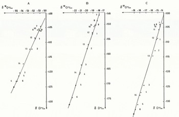
Fig. 2. The isotopic composition of water (1 to 6) and ice (7 to 14) during freezing experiments A, B, and C. The straight lines are the calculated slopes from the model. The black dots on the lines are the calculated ice values at 95% freezing. Water samples are denoted by circles, ice samples by crosses.
Three main points arise from Figure 2:
-
(1) A progressive impoverishment of the heavy isotopes in both the residual water and the ice layers is clearly visible during the course of freezing.
-
(2) Water and ice samples lie on a straight line. Using a least-square method, the slopes are respectively S = 4.37 ± 0.11 for the Antarctic melt-water, S = 5.99 ± 0.10 for the Arctic water, and S = 6.63 ± 0.17 for the alpine water. The correlation coefficients are always greater than 0.996.
-
(3) The slope for the Antarctic melt water is lower than that for the Arctic water which is lower than that for the alpine water, in relation to the initial isotopic composition.
The closed-system model developed by Reference Jouzel and SouchezJouzel and Souchez (1982) gives a slope S

where α is the equilibrium fracionation coefficient for deuterium, β the same coefficient for 18O, δi the δ value of the initial liquid for deuterium and ∆i the δ value of the initial liquid for 18O.
If we use α = 1.0208 (Reference ArnasonArnason, 1969) and β = 1.003 (Reference O’NeilO’Neil, 1968), the calculated slopes are respectively 4.32 for the Antarctic meltwater, 5.99 for the Arctic water and 6.27 for the alpine water. Experimental slopes are thus well in accordance with predicted slopes from the model.
During the experiments, excess water due to the phase change was allowed to escape and this can be considered as an output. Moreover, the water constituting the reservoir can be schematically divided into two parts: a region, close to the interface, of constant volume which is isotopically modified by the freezing process, and a region, away from the interface, which is isotopically unchanged and which can be considered as input; additional ideas are needed to take this division into account. It is worthwhile considering a natural reservoir with input and output and to develop a theory to examine whether the predicted slopes in an open-system model are the same as those in the closed-system model which we have presented previously (Reference Jouzel and SouchezJouzel and Souchez, 1982).
Theoretical Approach
At time t, NL is the number of moles in the liquid phase, NS the number of moles in the solid phase, NA the number of moles which have entered the system since t = 0 as input, NF the number of moles which have left the system since t = 0 as output, RS = (1 + δS) the isotopic ratio for D or 18O of the solid phase near the liquid-solid interface, RL = (1 + δL) the isotopic ratio of the liquid, RA = (1 + δA) the isotopic ratio of the input, and α SL the equilibrium fractionation coefficient between solid and liquid phases. Once formed, the solid has an isotopic composition which does not change in the course of time. At each step, the only isotope quantity (for D or 18)) brought to the solid phase is thus
Now for an open system
and for the isotopes
or

giving (on substituting dNL for its value in (1)

If we consider a constant input, a constant freezing rate, and an output proportional to the volume of remaining liquid, then

where A, S, and F are the respective coefficients for input, freezing, and output and N0 is the number of moles in the reservoir at time t = 0. Now, if k = NL/N0

This equation, applied to deuterium and 18O with the appropriate fractionation coefficient, gives the possibility by a step-by-step computation to calculate the δD and the δ18O of the remaining liquid phase and of the solid formed during the freezing process. Results indicate that, whatever the values of F/S and A/S may be, the two phases evolve almost linearly on a δD–δ18O diagram. The correlation coefficient is always more than 0.9999. Once this linearity between δD and δ18O is shown, the slope can be calculated in the following way: Let δL = δD and ∆L = δ18O for the liquid phase at time t. The slope for the solid phase is

From Equation (5), at time t = 0 (δL = δi and ∆L = ∆i), we obtain

This equation shows that the slope depends on (δA – δi) and (∆A – ∆i), the difference between the δ value of the input and that of the reservoir at time t = 0. In a natural reservoir, generally there is no reason for a change of input during the formation of this reservoir and during its subsequent freezing. Therefore, usually we shall have δA = δi and ∆A = ∆i. In this case, the expression of the slope reduces to

Equation (7) is independent of A, F, and S and almost identical to the equation obtained for the closed system. The slope will thus be the same for an open system as for the closed system when the input is not significantly different in its isotopic composition from that of the natural reservoir being considered.
Discussion
The open-system model developed above assumes a constant freezing rate but this is not the case in the experiments. However, the experimental results do not show a change of slope in the course of freezing in spite of the freezing-rate reduction. Moreover, the introduction of a time-dependent freezing rate in the model will make the computation more complicated but will have no effect on the slope.
If we now focus attention on the range between the ice (or residual water) value at 95% freezing and the initial value, the range in the experiments is less than that predicted by the closed-system model. The observed enrichment of the ice compared with the bulk of the liquid water depends on several parameters, particularly on the freezing rate and on the possible trapping of liquid during crystal growth. This dependency between the freezing rate and the obseved fractionations is discussed in Reference Posey and SmithPosey and Smith (1957), Reference O’NeilO’Neil (1968), and Reference ArnasonArnason (1969). As noted by Reference Posey and SmithPosey and Smith (1957), the observed separation will be less than the true value and the effect can be reduced by strong agitation and very slow freezing rates. Previous experiments without stirring led to correct slope values but to an even smaller range.
The following equation, equivalent to that which describes a Rayleigh process, was derived in the closed-system model:
where δi is the initial δ value of the reservoir and f is the liquid fraction with δL and δi expressed in per mil. From this equation, we can compute the apparent α and β values in the course of the three experiments. Apparent α and β values depend on the freezing rate which is about 1.9 cm h−1 at the beginning of each experiment and close to 0.8 cm h−1 at the end. In Figure 3, the apparent (α−1) values are plotted versus the apparent (β−1) values in the three experiments for different liquid fractions. A straight line joins the zero point where there is no fractionation to the point where (α − 1) and (β − 1) have their equilibrium values. From this Figure it is clear that the points are close to the straight line indicating that the slopes (αapp−1) and (βapp−1) in the experiments are not different from the equilibrium slope (α−1)/(β−1). It is quite probable that, for freezing rates encountered in Nature, the slope S is always a characteristic of the freezing process, even if apparent fractionation coefficients have values lower than their respective equilibrium values.
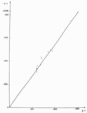
Fig. 3. Relationship between apparent fractionation coefficients in the freezing experiments. Equilibrium values are respectively: αeq −1 = 0.0208 and βeq −1 = 0.003.
The trapping of liquid water which subsequently freezes during crystal growth will lower the range but will have no effect on the slope since residual water samples and ice samples lie on the same straight line on a δ D−δ18O diagram.
Conclusion
The amount of fractionation which takes place during natural processes cannot be known. Even in the simplest of conditions, during, for example, the freezing of water in a closed system with isotopic equilibrium (allowing the application of the Rayleigh model), ice layers can be either isotopically enriched at the beginning of the process or isotopically impoverished at the end, compared with the initial reservoir. Under natural conditions the problem is complicated by non-equilibrium processes, the trapping of liquid water, and also input and output of water to and from the reservoir. Thus, it is not possible to show whether a refreezing process has taken place in a reservoir from the measurement of only one isotope (δD or δ18O). It is the δD−δ18O slope which is characteristic of the freezing process, on the other hand. This has been shown to be the case, both experimentally and theoretically, in the present paper.
Such a study may have implications for research concerning ice—bedrock interface problems and may shed some light on the origin of ice masses either at the earth surface or in the ground.
Acknowledgements
We are very grateful to R. Chiron for stable-isotope measurements.


