


1. Introduction
Satellite passive microwave sensors have provided information on areal sea-ice coverage, i.e. sea-ice concentration, for over 30 years. While these data can be sufficiently validated with higher-resolution visible, infrared and active microwave data, direct validation of satellite-derived sea-ice thicknesses (e.g. Reference Laxon, Peacock and SmithLaxon and others, 2003; Reference Giles, Laxon and RidoutGiles and others, 2008; Reference Zwally, Yi, Kwok and ZhaoZwally and others, 2008; Reference Kwok, Cunningham, Wensnahan, Zwally and YiKwok and others, 2009) or snow depth (Reference Markus, Cavalieri and JeffriesMarkus and Cavalieri, 1998) is more difficult. Nevertheless, the agreement between Envisat (Reference Giles, Laxon and RidoutGiles and others, 2008) and Ice, Cloud and land Elevation Satellite (ICESat; Reference Kwok, Cunningham, Wensnahan, Zwally and YiKwok and others, 2009) ice thickness retrievals in the Arctic is encouraging. For those reasons, a primary objective of a cruise to East Antarctica by the Australian icebreaker Aurora Australis in October 2003 (the Antarctic Remote Ice Sensing Experiment; ARISE) was to obtain large-scale information on the sea-ice conditions suitable for satellite validation (Reference MassomMassom and others, 2006). the strategy was a Lagrangian approach, and a drifting buoy array was set up, initially rectangular, 50 km ×100 km, in which we acquired extensive sea-ice information over a period of 3 weeks. the buoy array was deployed on 26 September 2003 and followed through to 12 October 2003. For comparison with AMSR-E-scale measurements it was divided into eight boxes of 25 km ×25 km. the philosophy of this approach was to be able to collect data in sufficient quantity for 25 km scales.
Snow depth on sea ice is operationally retrieved from the EOS (Earth Observing System) Aqua Advanced Microwave Scanning Radiometer (AMSR-E) sensor (Reference Comiso, Cavalieri and MarkusComiso and others, 2003). Regional and monthly snow depth distributions agree well with published in situ snow depth distributions (Reference Markus, Cavalieri and JeffriesMarkus and Cavalieri, 1998). A comparison with ASPeCt (Antarctic Sea Ice Processes and Climate) data (Reference Worby and AllisonWorby and Allison, 1999) shows that overall the agreement is quite good, although with a relatively wide scatter (Fig. 1) with the notable exception of East Antarctica. Similar results were found by Reference Worby, Markus, Steel, Lytle and MassomWorby and others (2008), who showed that in East Antarctica the passive microwave data underestimate snow depth by a factor of ∼2. This discrepancy is believed to be a result of ice roughness (Reference MarkusMarkus and others, 2006; Powell and others, 2006; Reference StroeveStroeve and others, 2006). the extent of the sea ice in the East Antarctic region is only ∼300 km, even in winter, so storms can cause significant disruption (e.g. deformation and ridging) all the way from the marginal sea-ice zone to the Antarctic coast, making the average roughness greater than in areas like the Weddell Sea.
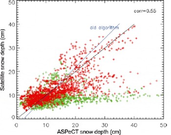
Fig. 1. Comparison of snow depth on sea ice derived from the SSM/I (Special Sensor Microwave/Imager) with in situ observations from the ASPeCt dataset. Data from the East Antarctic are shown in green. Data from elsewhere (Weddell Sea, Ross Sea, Amundsen/Bellingshausen Seas) are shown in red. the two lines represent the lines used for the current snow depth algorithm and from an updated regression using the ASPeCt data.
The utilization of ICESat data for the retrieval of sea-ice freeboard and thickness has been demonstrated for the Arctic (Reference Kwok, Cunningham, Wensnahan, Zwally and YiKwok and others, 2007; Reference Kwok and CunninghamKwok and Cunningham, 2008) and the Weddell Sea in the Antarctic (Reference Zwally, Yi, Kwok and ZhaoZwally and others, 2008). For the Arctic, the retrieval of freeboard from ICESat data compares well with data from ice mass-balance buoys (Reference Kwok, Cunningham, Zwally and YiKwok and others, 2007) and airborne laser data (Reference Kurtz, Markus, Cavalieri, Krabill, Sonntag and MillerKurtz and others, 2008). However, a comparison of ICESat-retrieved freeboards in the Antarctic with observations has not yet been undertaken.
In this paper, we develop a methodology to compare in situ measurements of snow and ice properties with satellite data from ICESat, AMSR-E and QuikSCAT. While daily, continuous information is available from AMSR-E and QuikSCAT, ICESat and in situ data are much more limited in space and time. To increase the number of coincident data points, we utilize information on sea-ice drift and sea-ice convergence to extrapolate the ICESat and in situ measurements in time.
2. Datasets
2.1. In situ data
During ARISE the snow and ice measurements were collected in three different ways:
Hourly ice and snow thickness measurements from the ship (ice observations). Ice and snow thickness are estimated from ice floes tipping on edge as the broken floes move along the icebreaker’s side as measured against a gauge (e.g. a buoy of known diameter near the water level). Additionally, the sea-ice conditions (concentration and thickness of various ice types) are estimated visually for a radius of ∼500m following the ASPeCt protocol (Reference Worby and AllisonWorby and Allison, 1999).
On 12 ice stations at different locations, detailed snow and ice properties along transects of 50–500m length were collected. Snow and ice thickness, as well as ice freeboard measurements, were taken every meter. Additionally, every 50m snow pits yielded information on snow stratigraphy and snow physical properties.
Random sampling, referred to as mini stations, using helicopters on floes within the buoy array were used to create representative large-scale statistics of snow depth and temperature. Each of these mini stations consisted of 20 snow depth and ice temperature measurements over level ice and 20 measurements over rough sea ice or at random locations. the distinction between smooth and rough ice was made by visual assessment. A total of 97 mini stations were utilized. the positions of the buoys also provide information on sea-ice drift and, through the calculation of areas for each of the eight boxes, information on sea-ice convergence/divergence.
The locations of all these measurements are shown in Figure 2. Note that these in situ measurements were single snapshots in time taken over the period of the ARISE campaign.

Fig. 2. Overview of measurements taken during the ARISE cruise. AMSR-E and QuikSCAT data are available daily in a 12.5 km and a 25 km grid, respectively. All other data are available for a specific day only.
2.2. Satellite data
Operational AMSR-E snow depth data are 5 day averages on a 12.5 km polar stereographic grid (Reference Comiso, Cavalieri and MarkusComiso and others, 2003). For better temporal coincidence we calculated daily snow depth using the AMSR-E Level 3 gridded brightness temperatures following the algorithm of Reference Markus, Cavalieri and JeffriesMarkus and Cavalieri (1998). the algorithm uses modified coefficients developed for AMSR-E data to ensure consistency. the functional form of the algorithm is
where h s is snow depth and GRice is the spectral gradient ratio of the AMSR-E 19 and 37 GHz vertical-polarization channels corrected for variations in sea-ice concentration. the locations are indicated as black crosses in Figure 2.
Daily QuikSCAT backscatter data at both vertical and horizontal polarization gridded to a 25 km grid were obtained from Brigham Young University (http://www.scp.byu.edu/;Long, 2000). These data are used below as a proxy for large-scale surface roughness. the locations are indicated as purple plus signs in Figure 2.
At the mini stations, snow depths were recorded separately for smooth and for rough sea ice. We did not, however, record an estimate of the areal fraction of those two ice conditions. Gridcell fractions of rough and smooth ice are therefore calculated using QuikSCAT data. Similar to the calculation of the thin-ice fraction, two tie points are used to obtain the fractions of rough ice and smooth ice. A vertical polarization backscatter of −20 dB is chosen to be representative of smooth ice, and a backscatter of −13 dB representative of rough ice (Reference Long and DrinkwaterLong and Drinkwater, 1999).
ICESat sea-ice products are elevation and sea-ice roughness. the sea-ice roughness is determined from the width of the return waveform. the ICESat dataset used is release 428 with elevation corrections for moderately saturated waveforms applied. It is necessary to first filter out elevation data that are significantly affected by atmospheric scattering, such as from clouds or blowing snow. Scattering increases the path length traveled by the photons, which biases the retrieved elevation. These biased elevation data are identified from instrument- and waveform-derived parameters and removed using filtering parameters similar to those described by Reference Zwally, Yi, Kwok and ZhaoZwally and others (2008). Additionally, the effects of tides, atmospheric pressure loading and geoid variations have been removed from the ICESat elevation data following the method described by Reference Zwally, Yi, Kwok and ZhaoZwally and others (2008). the subtraction of these parameters from the elevation data provides a relative elevation, h r. Freeboard, h f , is then found from the relative elevation data through subtraction of the local sea surface elevation termed the sea surface tie point, h tp:
Details of the retrieval of freeboard are given in section 4.2 below.
Sea-ice roughness can also be determined from the standard deviation in elevation over 25 km intervals (Reference Kwok, Cunningham, Zwally and YiKwok and others, 2007). In the following the latter is referred to as σ 25. the ICESat tracks with valid elevation data are indicated by gray asterisks in Figure 2.
3. Methodology
Figure 2 shows poor overlap between the ICESat and the in situ data. We use ice-drift information obtained from the drifting buoys to extrapolate ICESat and in situ observations to other days. Analysis of the drifting buoy locations has shown that the ice in the area drifted about 0.1 ˚ d − 1 to the west, with negligible meridional drift. the assumption is that snow and freeboard conditions for those ice floes measured did not change significantly over the campaign period. the only change is in the fraction of thin ice for each gridcell, caused by ice divergence. Since this extrapolation in time is imprecise, we averaged the extrapolated data as well as the daily AMSR-E and QuikSCAT data to a latitude/longitude grid spaced at 0.5 ˚ in latitude and 1 ˚ in longitude. For the latitude range of this campaign this corresponds to a grid size of roughly 55.5 km ×47 km. All further analysis is done in this grid.
Consideration is required to take account of the fact that ice stations as well as mini stations occurred on thicker ice only. Obviously no in situ observations can be taken over thin sea ice. For thin ice the snow depth is generally minimal and the ice is relatively smooth. It is therefore necessary to account for the thin-ice fraction within the gridcells to avoid a bias towards the conditions on thicker ice. For some days aerial photography from helicopters could be utilized (Reference Worby, Markus, Steel, Lytle and MassomWorby and others, 2008), but these data are too limited for the scope of this paper. Therefore, we use AMSR-E data to obtain an estimate of the fraction of thin ice compared to thick ice within the gridcell. Reference Martin, Drucker, Kwok and HoltMartin and others (2004) and Reference Tamura, Ohshima, Markus, Cavalieri, Nihashi and HirasawaTamura and others (2007) have shown that differences in the polarization of microwave radiances can be used to derive the thickness of thin sea ice. Here, we follow Reference Martin, Drucker, Kwok and HoltMartin and others (2004), who calculate the thin-ice thickness using R = T B(37V)/T B(37H), where T B(37V) and T B(37H) are the AMSR-E brightness temperatures at 37 GHz vertical (V) and horizontal (H) polarization, respectively. Instead of calculating a thin-ice thickness, the fraction of thin ice is calculated using two tie points. A value of R = 1.05 represents 100% thick ice, and a value of R = 1.3 represents 100% thin ice. A value of 1.05 corresponds to the maximum ice thickness retrievable by Reference Martin, Drucker, Kwok and HoltMartin and others (2004); R asymptotically reaches its minimum at a value of 1.05. A value of 1.3 corresponds to an ice thickness estimate of ∼2 cm and an areal fraction of 100% thin ice. For the time and area of this campaign the thin-ice fraction was ∼10% with a range from 0% to 20%.
Using these sources of additional information, snow depth for each gridcell using mini stations is calculated using
where F thick and F rough are the fractions of thick and rough ice, respectively, and h s(thin) is the snow depth of thin ice, which was set to zero. Gridded snow depth for the ice stations is calculated the same way, although for the ice stations no distinction between rough and smooth ice is made, assuming that the transects are a valid representation of the average ice and snow conditions over thick ice.
A good check to assess the methodology and the validity of these steps is the agreement between ice-station and mini-station data after extrapolation and gridding shown in Figure 3. the dotted lines indicate the 5 cm differences. While some data show good agreement, others differ widely. Large differences are an indication that either the mini-station or ice-station data were not representative of the gridcell or that our assumptions do not hold for those cases. To be conservative, in the following we use only those values where the difference between ice stations and mini stations is <5cm. This number is somewhat arbitrary, but 5 cm corresponds to the noise level in AMSR-E snow depth retrieval.

Fig. 3. Mini-station snow depth versus ice-station snow depth. Dotted lines indicate 5 cm differences.
4. Analyses
4.1. Surface roughness
The large number of individual snow and ice measurements at the ice stations enables us to estimate the standard deviation for snow depth, ice thickness and freeboard for each station. Since surface elevation is the sum of snow depth and freeboard, the corresponding standard deviations are added to calculate an ice-station-elevation standard deviation. These data are compared with the roughness and standard deviation estimates, σ 25, from ICESat and with backscatter values from QuikSCAT in Figure 4. Ice-station data and σ 25 data show similar trends and show good agreement in actual values, except for ice-station values >22cm where ICESat σ 25 shows almost constant values of ∼17 cm (Fig. 4a). No correlation can be seen between ice-station standard deviation and ICESat roughness derived from the waveform (Fig. 4b). ICESat σ 25 also shows good correlation with QuikSCAT backscatter (Fig. 4c), although the plot suggests ICESat σ 25 saturates at ∼35 cm. Similar to Figure 4b, ICESat roughness shows no correlation with the QuikSCAT data (Fig. 4d).

Fig. 4. Scatter plots of (a) ICESat elevation standard deviation, σ 25, vs ice-station standard deviation, (b) ICESat roughness vs ice-station standard deviation, (c) ICESat σ 25 vs QuikSCAT vertical-polarization backscatter, and (d) ICESat roughness vs QuikSCAT vertical-polarization backscatter.
4.2. Sea-ice freeboard
The main limiting factor in freeboard retrievals from ICESat data is the identification of suitable sea surface height tie points. We needed to develop a method that identifies sea surface height tie points using ICESat data alone in order to be able to retrieve freeboard for the entire Antarctic basin. Using near-coincident (<3 hour temporal separation) Moderate Resolution Imaging Spectroradiometer (MODIS) and ICESat data for the entire Southern Ocean, we first identified areas of open water and thin ice within the ice pack using thresholds in the MODIS data. These provide a reference set of a total of 905 ICESat sea surface height tie points. By comparing this reference h tp dataset with the 25 km standard deviation of h r, σ 25, we found a linear relationship between the two (shown in Fig. 5). A similar linear relationship between σ 25 and sea surface elevation was also found for the Arctic and forms the starting point for a freeboard retrieval algorithm described by Reference Kwok, Cunningham, Zwally and YiKwok and others (2007). There is, however, some scatter in the data which is most likely due to atmospherically contaminated shots and also thick ice points erroneously identified as sea surface tie points. the fitted lines are derived using a robust fit procedure (iteratively reweighted least squares with a bisquare weighting function) to reduce the impact of these outliers, with ∼90% of the points falling within 7 cm of the fitted lines. the properties of the fitted lines change only slightly with season. the y-intercept of the May–June 2005 fitted line is near zero; however, we may expect the y-intercept should be closer to the ∼2 cm noise level of ICESat (Reference Kwok, Zwally and YiKwok and others, 2004). Potential errors in the fitted line such as this may cause errors in the retrieved freeboards; but the effect should not be significant because the fitted lines are only a starting point for the freeboard retrieval method described below.

Fig. 5. Relationship between the ICESat 25 km standard deviation in elevation, σ 25, and the ICESat elevation of sea surface height tie points identified using MODIS data, h tp, for (a) September to October 2003 and (b) May to June 2005. the dashed lines represent the ±7 cm area where sea surface tie points are taken to be located in the retrieval algorithm.
The linear relationship between h tp and σ 25 forms the starting point for the identification of sea surface tie points by providing a narrow range of data with which to search for suitable tie points. We expect the sea surface tie points to satisfy the following criteria:
h r should be within 7 cm of the estimated sea surface tie point value, h est, found using the local value of σ 25 and the parameters of the fitted line from Figure 5. the value of 7 cm is ∼1.5 times the standard deviation of the difference of the points from the fitted line.
h r should be within 5 cm of other nearby sea surface tie points. the value of 5 cm is the estimate of the uncertainty in the sea surface height from the tie points found using ICESat.
h r should be the lowest value within a profile of unbiased (i.e. not contaminated by atmospheric scattering) elevation measurements.
Our method for finding the local value of h tp for all Antarctic ICESat sea-ice data which satisfy the above criteria is as follows: For each ICESat point find σ 25 and calculate h est; take h tp to be the average of the lowest three values of h r within 12.5 km and ±7cm of h est. If no points satisfy the criteria then h tp is not found and freeboard is not retrieved. the advantage of this method is that the sea surface tie points are selectively identified from within the surrounding sea-ice cover. This method also further reduces the effect of unreliable atmospherically scattered elevation measurements.
To determine the validity of the ICESat retrieved freeboards using this method, we compared the results to in situ freeboards from the ARISE dataset. the ICESat data consist of the averaged freeboard values for each individual ICESat overpass (taken between 25 September and 17 October 2003) within each of the ARISE gridcells. the in situ freeboards for each gridcell are taken as the mean snow depth plus ice freeboard from the ice stations. the results are shown in Figure 6. the data have a correlation of 0.6, with some of the scatter likely due to the extrapolation of the data in space and in time, and due to the spatial variability of the ice freeboard and snow depth within the gridcell. the mean difference between the datasets is small, with ICESat having an average freeboard 1.8 cm higher than the ARISE dataset. the small mean difference is particularly important as it suggests that the method used to retrieve the sea surface tie points is not significantly biased and that the overall large-scale retrieved ICESat freeboard values are comparable to the observed in situ data.

Fig. 6. Comparison between the ICESat-derived freeboard and ice-station freeboard from the ARISE dataset. Freeboard is taken to be the height of the ice plus the snow layer above the water level.
4.3. Snow depth
Previous studies have suggested that AMSR-E underestimates snow depth in areas with a high fraction of rough sea ice (Reference MarkusMarkus and others, 2006; Reference MaslanikMaslanik and others, 2006;Reference Worby, Markus, Steel, Lytle and MassomWorby and others, 2008). the following comparison attempts to utilize ICESat data to account for sea-ice roughness in the AMSR-E snow depth algorithm. ICESat σ 25 is used for this comparison rather than QuikSCAT because the QuikSCAT backscatter may be influenced by changes in snow and ice physical properties in addition to the roughness. Further study is required to better interpret the QuikSCAT signal, especially when applied automatically. A comparison of AMSR-E snow depth with station snow depth (Fig. 7) shows two clusters: one with data points close to the diagonal and one with data points where the station snow depths are considerably greater. Coincident ICESat σ 25 data show correspondingly low values for the data close to the diagonal (σ 25 < 15 cm; blue and green dots) and high values where the station data are significantly greater than the AMSR-E snow depth (σ 25 > 15 cm; brown and purple dots). the differences between AMSR-E snow depth and ARISE snow depth for small σ 25 values are within the uncertainties of the data: ∼5 cm for both datasets. For large σ 25 values the differences in snow depth are outside the 5 cm error. This suggests that ICESat σ 25 may be used to adjust passive microwave snow depth retrievals to account for sea-ice roughness.

Fig. 7. AMSR-E snow depth vs ice-station and mini-station snow depth. ICESat elevation standard deviation, σ 25, is indicated by the color scale.
Using multiple linear regression we obtain a relationship
for snow depth, h s:
where GRice is the AMSR-E spectral gradient ratio corrected for sea-ice concentration variations, as used in the current AMSR-E snow depth routine. Comparison with ARISE in situ snow depth gives a correlation coefficient of 0.84 with a mean difference of 2.3 cm and a negligible bias (Fig. 8). While the results look encouraging, it is important to note that the data are from a limited region and a limited period so the results cannot necessarily be directly transferred to other areas or other seasons.

Fig. 8. Combined ICESat/AMSR-E snow depth vs ice-station and mini-station snow depth.
5. Summary and Conclusions
A focus of the ARISE campaign was to establish an in situ dataset optimized for the validation of satellite data. We developed a methodology to compare in situ measurements of sea-ice and snow properties with satellite data. Utilizing information on sea-ice drift and sea-ice divergence from buoys, and sea-ice types from AMSR-E and QuikSCAT we are able to extrapolate in situ measurements as well as ICESat data in space and in time and thus significantly increase the number of data points available for comparison. In the datasets before extrapolation there were virtually no coincident ICESat and in situ data. the validity of the extrapolation procedure was assessed by comparison of two types of in situ measurements (ice stations and mini stations) that were initially not coincident. Only data that agreed to within 5 cm were used for comparison with the satellite data.
The dataset was used to validate a method for deriving freeboard from ICESat data over Antarctic sea ice. the results show that ICESat freeboard estimates have a mean difference of 1.8 cm when compared with the in situ data and a correlation coefficient of 0.6. While the results are only compared with ship data in East Antarctica, the method should also be applicable to the entire Southern Ocean. This will be studied in the future. We furthermore saw good agreement between in situ roughness and ICESat elevation standard deviation, σ 25.
The comparisons also confirmed the underestimation of AMSR-E snow depth for rough sea-ice areas. the addition of a roughness term, using ICESat, into the AMSR-E snow depth retrieval can enhance the snow depth retrievals significantly. Snow depth retrievals using a combination of AMSR-E and ICESat data agree with in situ data with a mean difference of 2.3 cm and a correlation coefficient of 0.84 with a negligible bias. More work is needed to expand the correction scheme to hemispheric snow depth retrievals. the better spatial and temporal coverage of QuikSCAT compared to ICESatmake it an ideal candidate for roughness correction, but the distinction between backscatter variations caused by different levels of roughness and variations caused by changes in snow and sea-ice properties needs further study.
Acknowledgements
We gratefully acknowledge the professional support of Captain Pearson, the officers and crew of the RSV Aurora Australis, and the helicopter pilots and crew. This work was supported by the Australian Government’s Cooperative Research Centres Programme through the Antarctic Climate and Ecosystems Cooperative Research Centre (ACE CRC). It was carried out as part of AAS project 2298 and NASA’s AMSR-E Validation Program (http://eospso.gsfc.nasa.gov/validation/index/php) through NRA-OES-03, and contributes to AAS project 3024. Thanks are also extended to the expeditioners traveling to Casey for their help in collecting the snow data.


