


1. INTRODUCTION
The Greenland ice sheet is losing mass at an increasing rate (Kjeldsen and others, Reference Kjeldsen2015), almost equally distributed between an increase in the surface melt during summer and an acceleration of flux to the ocean through marine-terminating outlets (Van den Broeke and others, Reference Van den Broeke, Enderlin, Howat and Noël2016; van den Broeke and others, Reference van den Broeke2017). This latter contribution has been shown to be mostly controlled by processes acting at the front of glaciers, where the ice meets the ocean (e.g. Rignot and others, Reference Rignot, Koppes and Velicogna2010). For land-terminating glaciers in Greenland, the only process that can modulate their ice dynamics over short-term periods of a few decades is changes in their basal conditions caused by changes in surface run-off. Faster velocities for these land-terminating glaciers could bring more ice into the ablation area and in turn increase the loss by surface melt.
Even though the ability of surface meltwater to modulate the flow of alpine glaciers at diurnal and seasonal timescale has been known for a long time (e.g. Lliboutry, Reference Lliboutry1958; Iken and Bindschadler, Reference Iken and Bindschadler1987; Mair and others, Reference Mair2003), it is only relatively recently that this process was shown to operate also for larger ice masses such as Greenland outlet glaciers (Zwally and others, Reference Zwally2002). These observations on Greenland outlet glaciers show that changes in ice flow are strongly linked to changes in surface run-off. However, studies found that increased melt can cause both speed-ups in ice flow (e.g. Zwally and others, Reference Zwally2002; Shepherd and others, Reference Shepherd2009; Bartholomew and others, Reference Bartholomew2010), as well as slow-downs (e.g. Tedstone and others, Reference Tedstone2015). This shows that the relation between the amount of run-off and ice flow speed is complex and variable in time and space, reflecting the evolution of the basal drainage system during the melt season (e.g. Bartholomew and others, Reference Bartholomew2010; Schoof, Reference Schoof2010).
Since the mid-1990s, surface melt in Greenland has increased both in amplitude and extent (Hanna and others, Reference Hanna2005; Fettweis and others, Reference Fettweis2013; Poinar and others, Reference Poinar2015; Van den Broeke and others, Reference Van den Broeke, Enderlin, Howat and Noël2016), producing more water with the potential to reach the bed at higher elevation. Based on observations of current surface strain rates, Poinar and others (Reference Poinar2015) conclude that this surplus of water produced above a critical elevation of ~1600 m will likely flow in surface streams until it reaches existing moulins much further downstream and will, therefore, not influence upstream basal conditions. Similar conclusions are drawn by Stevens and others (Reference Stevens2015) regarding the capacity of high elevation supraglacial lakes to drain, as the creation of new surface-to-bed connections, may be limited. On the contrary, recent results by Hoffman and others (Reference Hoffman2018) and Christoffersen and others (Reference Christoffersen2018) suggest that supraglacial lake drainage could allow an upstream propagation of moulins and allow water to reach bed at higher elevations. For the same study area as that of Poinar and others (Reference Poinar2015), Yang and Smith (Reference Yang and Smith2016) have observed that almost all the run-off produced above 1600 m enters moulins at the same elevation interval, suggesting that moulins are more common above this elevation than previously reported.
Here, motivated by these present-day observations of the crevasse and moulin distributions (Poinar and others, Reference Poinar2015; Stevens and others, Reference Stevens2015; Yang and Smith, Reference Yang and Smith2016), we develop a modelling framework which couples a hydrology and an ice flow component to simulate the evolution of the extent of the crevassed area of outlet glaciers in Greenland in a warming climate. We first explain the various components of the coupled model, then describe the numerical experimental setups of our synthetic experiments and finally, we present our predictions of how far inland ice flow speed up will reach using multi-decadal simulations.
2. COMPONENTS OF THE COUPLED MODEL
The numerical experiments presented in this work aim at coupling a number of processes acting at the glacier surface, in the glacier itself and at its base. This section presents in detail all the models or parameterizations for surface mass balance, ice flow, basal friction, glacier geometry evolution, supra-, intra- and sub-glacial hydrology and crevasse and moulin opening. The processes accounted for in the model as well as their coupling are schematized in Figure 1 and on the flow chart in Figure 2. All values for the parameters of the different components of the model are given in Table 1.
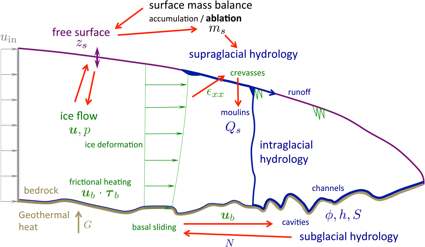
Fig. 1. Processes accounted for in the model and their coupling indicated by red arrows. In black the surface mass balance, in blue the supra-, intra- and sub-glacial hydrology, in green the deformational and sliding components of ice flow and in purple the evolution of the upper free surface. A constant inflow velocity u in = 18 m a−1 is imposed on the left boundary of the model domain.
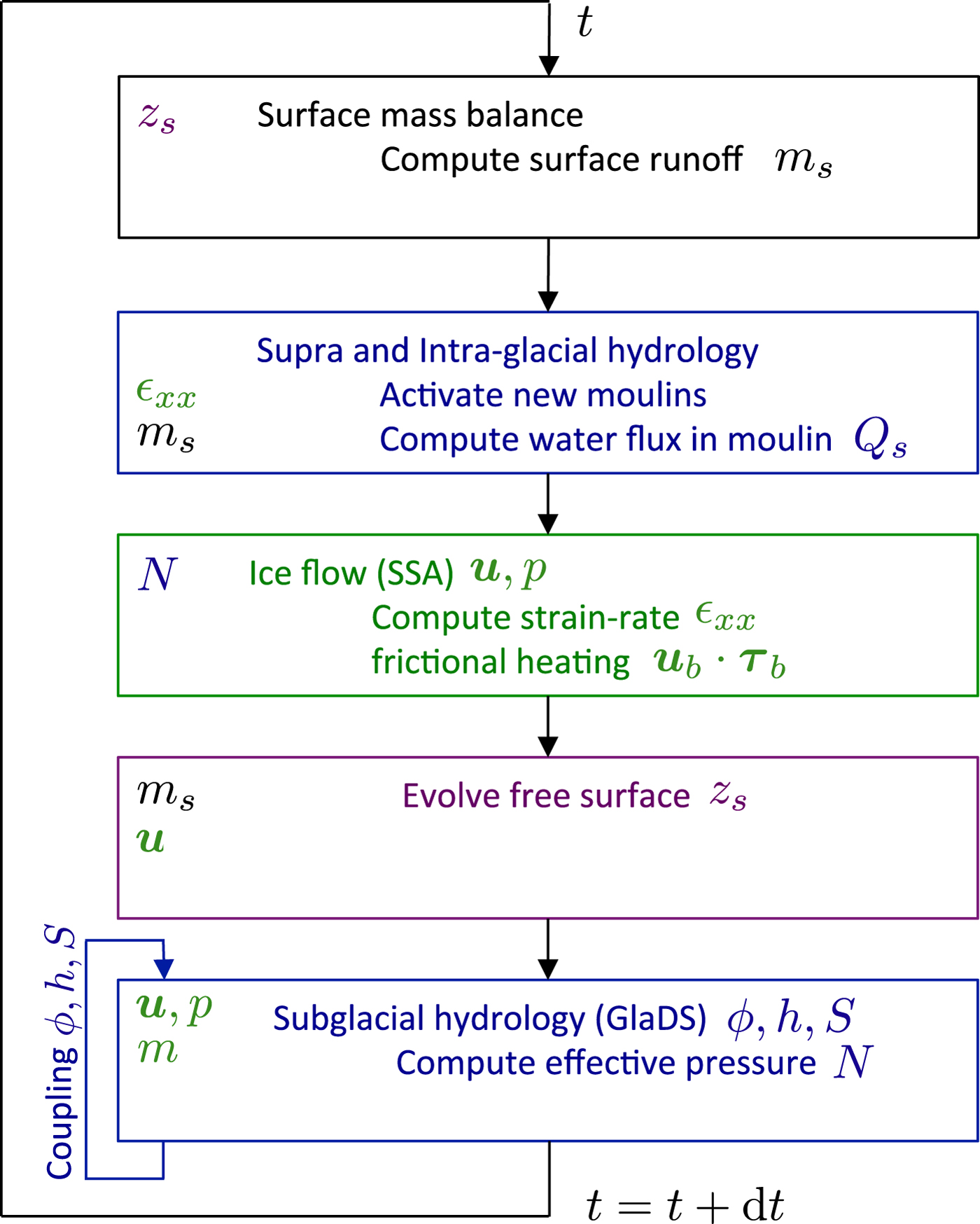
Fig. 2. Flow chart for one time step of the coupled model indicating input (on the left) and output (on the right) variables. The same colour code as in Figure 1 is used. The coupling between the hydrology variables (last step) is described in detail in the Appendix.
Table 1. Values of the parameters used in this study

All these equations have been implemented in the open-source finite element code Elmer/Ice (Gagliardini and others, Reference Gagliardini2013).
2.1 Glacier geometry
The geometry of the glacier considered in this paper, despite being synthetic, is representative of a land-terminating glacier in Greenland. The bed is assumed to be flat at an elevation b = 500 m a.s.l. The glacier domain is 150 km long and 10 km wide, with periodic boundary condition on the sides. An initial geometry is obtained by spinning-up the coupled model until a seasonally periodic solution is obtained (see Fig. 3). All perturbation experiments start from this initial seasonally-steady geometry.
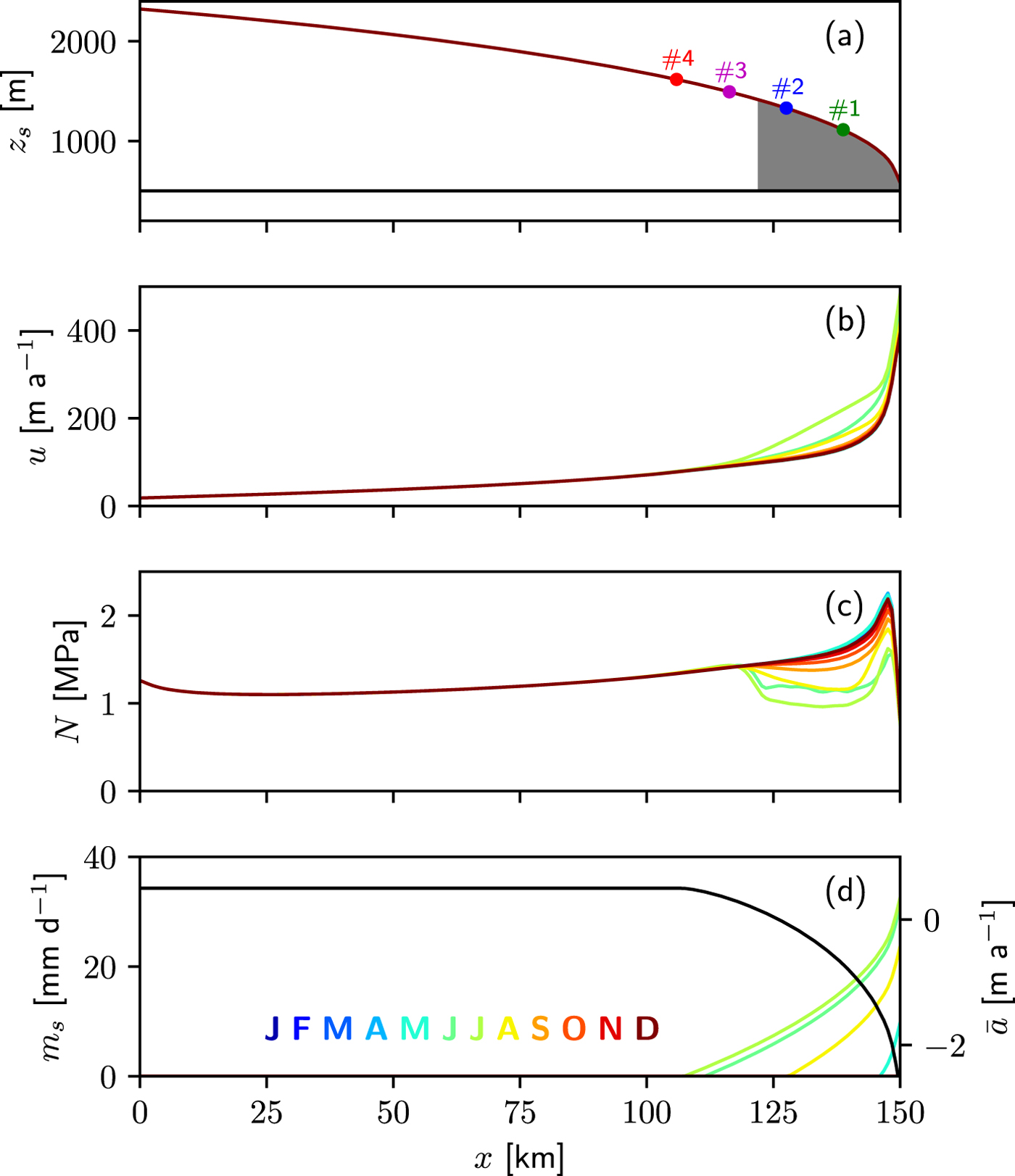
Fig. 3. Initial state: laterally-averaged (a) surface elevation z s, (b) velocity u, (c) effective pressure N and (d) surface runoff m s (m w.e.) for the 12 months of the year (colour). In (d), the black line represents the annual surface mass balance  $\bar {a}$ (m ice eq., right axis). The grey area in (a) corresponds to the initial crevassed area in which moulins are activated. Seasonal variations of the surface elevation are invisible at this scale. The colored dots in (a) give the position of four sites used to present subsequent results at respectively 11, 22, 33 and 44 km from the glacier margin.
2.2 Surface mass balance
Following Hewitt (Reference Hewitt2013), the dependency of run-off m s (m w.e.) on surface elevation z s and time t is described using the following parameterization:
 $$\eqalign{m_{\rm s}(z_{\rm s},t) & = \max \left[ {0,\displaystyle{{r_{\rm m} + r_{\rm s}s_{\rm m}(t)} \over 2}} \right.\left( {\tanh \left( {\displaystyle{{d(t) - d_{{\rm spr}}} \over {\Delta d}}} \right)} \right. \cr & \quad \quad \quad \left. {\left. { - \tanh \left( {\displaystyle{{d(t) - d_{{\rm aut}}} \over {\Delta d}}} \right)} \right) - r_{\rm s}z_{\rm s}} \right]}, $$
where d(t) is the day of the year at time t and z s is the surface elevation. The only parameter which is varied for different model scenarios is s m(t), which gives the altitude at which melt reaches the value r m. The parameter s m(t) will, therefore, encompass all climate changes for the perturbation experiments. The values of all other parameters, r m, r s, Δd, d spr and d aut, are constant and given in Table 1.
For the upper surface evolution (see below equation (8)), the surface mass balance is given as the difference between accumulation (c), assumed constant and uniform and the ablation, i.e. the surface run-off in m ice eq., reads:
 $$a(z_{\rm s},t) = c - \displaystyle{{\rho _{\rm w}} \over {\rho _{\rm i}}}m_{\rm s}(z_{\rm s},t),$$
where ρ i and ρ w are ice and water density, respectively.
Accumulation and parameters in the surface melt function (1) have been calibrated to reproduce the surface mass-balance dependence on elevation for Greenland given by the regional climate model MAR using ERA-Interim reanalysis from 1979 to 2014 (Fettweis and others, Reference Fettweis2017). The yearly-averaged surface mass balance used to construct the initial state is depicted in Figure 3d as a function of distance to the front (black curve).
Note that a larger amount of surface melt than the runoff m s(z s, t) might be produced at the surface of the glacier but this surplus of water is assumed to percolate and refreeze or form a water reservoir in the firn so that it is assumed not to contribute to change in surface elevation and not to reach the base of the glacier over the study period.
2.3 Ice flow
Ice flow will be modulated primarily by the effective pressure at the base of the glacier N = p − p w, with p and p w the ice and water pressures, respectively, whereas changes in the glacier surface elevation z s will only have a significant effect on a timescale longer than considered here.
The ice flow is solved using the Stokes asymptotical equations for ice streams under the Shallow Stream Assumption (SSA). Using membrane stresses (Greve and Blatter, Reference Greve and Blatter2009), the vertically integrated stress equilibrium reads:
 $$\left\{ \matrix{2\displaystyle{{\partial T_{xx}} \over {\partial x}} + \displaystyle{{\partial T_{yy}} \over {\partial x}} + \displaystyle{{\partial T_{xy}} \over {\partial y}} - \tau _{bx} = \rho _igH\displaystyle{{\partial z_{\rm s}} \over {\partial x}} \hfill \cr 2\displaystyle{{\partial T_{yy}} \over {\partial y}} + \displaystyle{{\partial T_{xx}} \over {\partial y}} + \displaystyle{{\partial T_{xy}} \over {\partial x}} - \tau _{by} = \rho _igH\displaystyle{{\partial z_{\rm s}} \over {\partial y}} \hfill} \right.$$
where  $T_{xx} = 2 \bar {\eta } \partial u / \partial x$, $T_{yy} = 2 \bar {\eta } \partial v / \partial y$, $T_{xy} \!=\! \bar {\eta } (\partial u / \partial y \!+\! \partial v / \partial x$), H = z s − b is the ice thickness and
  $${\bi u} = (u,{\mkern 1mu} v)$$ the horizontal velocity vector.
The vertically averaged effective viscosity  $\bar {\eta }$ reads:
 $$\bar \eta = \displaystyle{1 \over 2}d_{\rm e}^{ - (1 - 1/n)} H\bar A^{ - 1/n},$$
with  $\bar {A}$ the vertically averaged fluidity, n the Glen's flow law exponent and the reduced effective strain rate
 $$d_{\rm e}^2 = \left( {\displaystyle{{\partial u} \over {\partial x}}} \right)^2 + \left( {\displaystyle{{\partial v} \over {\partial y}}} \right)^2 + \displaystyle{{\partial u} \over {\partial x}}\displaystyle{{\partial v} \over {\partial y}} + \displaystyle{1 \over 4}\left( {\displaystyle{{\partial u} \over {\partial y}} + \displaystyle{{\partial v} \over {\partial x}}} \right)^2.$$
The ice pressure p simplifies to the overburden pressure and reads:
 $$ p = \rho_{{\rm i}} g H .$$
 In (3), the basal shear stress  $${\bi \tau }_{\rm b} = (\tau _{{\rm b}x},{\mkern 1mu} \tau _{{\rm b}y})$$ is linked to the sliding velocity ub = u using the pressure-dependent friction law proposed by Schoof (Reference Schoof2005) and Gagliardini and others (Reference Gagliardini, Cohen, Råback and Zwinger2007):
 $${\bi \tau }_{\rm b} + \displaystyle{{CN_ + \vert {\rm }{\bi u}_{\rm b} \vert ^{(1/n - 1)}} \over {{\left( { \vert {\rm }{\bi u}_{\rm b} \vert + C^nA_{\rm s}N_ + ^n } \right)}^{1/n}}}{\mkern 1mu} {\rm }{\bi u}_{\rm b} = 0.$$
The friction law depends on the without-cavity sliding parameter A s, the Iken's bound parameter C and the Glen's flow law exponent n. For large effective pressure N and/or small sliding velocity u b, this friction law is equivalent to a Weertman-type friction law, i.e. τ b ≈ (u b/A s)1/n. At the opposite extreme, for low effective pressure and/or high velocity, it reduces to a Coulomb-type friction law τ b ≈ CN. Following Hewitt (Reference Hewitt2013) and Koziol and Arnold (Reference Koziol and Arnold2018), the effective pressure is replaced by N + = max (0, N) to avoid negative effective pressure in the friction law that can be obtained from the sub-glacial hydrology model.
For the other glacier boundaries, periodic conditions for velocity and pressure are assumed on the sides of the domain, a constant velocity u in is imposed on the inflow boundary and a no-stress condition is applied at the ice front.
2.4 Geometry evolution
The evolution of the glacier geometry is governed by the ice flow velocity and the surface melt m s. Using the SSA, the glacier geometry evolution is given as the evolution of ice thickness:
 $$\displaystyle{{\partial H} \over {\partial t}} + \nabla \cdot (H{\rm }{\bi u}) = a,$$
where u = (u, v) is the mean horizontal velocity vector. Surface elevation is then simply derived as z s(x, t) = b(x) + H(x, t). The only boundary condition imposed for the ice thickness is its periodicity on the sides of the domain. Together with the stress boundary conditions, this means that the ice thickness at the inflow boundary and at the front is allowed to evolve freely. However, note that the frontal position is held fixed, i.e. an ice cliff occurs for a glacier advance and zero ice thickness for a glacier retreat. Due to the initial geometry and the relatively short studied period, this latter case was never reached.
2.5 Water flow
This section presents how the water produced by ice melt on the glacier surface is routed at the surface, in the glacier and at the base of the glacier until it reaches the margin. As explained below, subglacial hydrology is influenced by the ice flow through longitudinal strain rate via the creation of new crevasses and moulins and through sliding velocity via its impact on the opening of basal cavities. Moreover, the water production at the surface given by (1) is a function of the surface elevation z s.
Regarding the supra-glacial hydrology model, the produced surface meltwater is instantaneously routed to the closest activated moulin located downstream. As a consequence, the model does not account for any supraglacial storage (lakes or within the firn) and the water produced at an elevation lower than the elevation of the lowest moulin reaches the glacier front without entering any moulin. Also, when a new moulin is activated, moulins located just downstream of this new moulin will receive less water than before its activation. The surface water input in activated moulin k is given as:
 $$Q_{\rm s}^k (t) = \int_{{\rm {\cal A}}_k} {m_{\rm s}} (z_{\rm s},t){\rm }{\rm d}\,{\rm {\cal A}},$$
where  ${\cal A}_k$ is the surface area which drains into moulin k. Note that ${\cal A}_k = {\cal A}_k(t)$, such that the surface connected to a moulin can decrease if new moulins at higher elevations are activated.
Initially, 200 moulin positions are randomly distributed over the domain with higher density at lower elevation (Hewitt, Reference Hewitt2013; Yang and Smith, Reference Yang and Smith2016). A moulin is only activated if it belongs to the crevassed area, otherwise, it will not allow any water to drain. Following Poinar and others (Reference Poinar2015), it is assumed that crevasses open where the maximal tensile strain rate has reached the crevasse criterion ε th = 0.005 a−1. As the ice temperature is assumed constant and homogeneous, a more physically founded criterion relying on stress should give similar results. Moreover, due to the simple glacier geometry adopted here (limited cross-flow variation) and due to the SSA formulation, this criterion can be stated as ∂u/∂x ≥ ε th. No mechanisms allowing for crevasse closing are accounted for so that the crevassed area can only increase with time.
For the englacial hydrology model, it is assumed that the water reaches the bed at the horizontal location of the moulin, i.e. moulins are assumed to be perfectly vertical and with infinite conductivity, but with the potential to store water, such that the discharge out of moulin k is
 $$Q_{\rm m}^k = - \displaystyle{{A_{\rm m}^k } \over {\rho _{\rm w}g}}\displaystyle{{\partial \phi } \over {\partial t}} + Q_{\rm s}^k ,$$
with  $A^k_{{\rm m}}$ the moulin cross-sectional area and ϕ the hydraulic potential at the bed, defined as
 $$ \phi = \phi_{{\rm m}} + p_{{\rm w}} ,$$
with the elevation potential ϕ m = ρ wgb. All moulins are further assumed to have the same constant cross-sectional area so that  $A_{{\rm m}}^k = A_{{\rm m}} = 10\,{\rm m}^2$. Water input for the sub-glacial hydrology model is composed of the discharge out of all activated moulins $Q_{{\rm m}}^k$ plus the distributed melt from geothermal heat flux G and frictional heating, given as
 $$m_{\rm b} = \displaystyle{{G + \vert {\rm }{\bi \tau }_{\rm b} \cdot {\rm }{\bi u}_{\rm b} \vert } \over {\rho _{\rm i}L}}.$$
The sub-glacial hydrology follows the Glacier Drainage System model GlaDS (Werder and others, Reference Werder, Hewitt, Schoof and Flowers2013). Exactly the same set of equations as in Werder and others (Reference Werder, Hewitt, Schoof and Flowers2013) has been implemented in Elmer/Ice. These equations are summarized here and technical details regarding their implementation in Elmer/Ice is given in the Appendix. For a complete description of the GlaDS model, the reader should refer to Werder and others (Reference Werder, Hewitt, Schoof and Flowers2013).
The sub-glacial drainage system couples distributed (water sheet consisting of linked cavities) and channelized water flow. The whole drainage system is described by the hydraulic potential ϕ at the bed, the sheet thickness h and the channel cross-sectional area S. The evolution of these three variables are given by the following set of four equations
 $$\displaystyle{{e_{\rm v}} \over {\rho _{\rm w}g}}\displaystyle{{\partial \phi } \over {\partial t}} - \nabla \cdot {\rm }{\bi q} + w_{\rm s} - v_{\rm s} - m_{\rm b} = 0,$$
 $$\displaystyle{{\partial Q} \over {\partial s}} + \displaystyle{{\Xi - \Pi } \over L}\left( {\displaystyle{1 \over {\rho _i}} - \displaystyle{1 \over {\rho _w}}} \right) - v_{\rm c} - m_{\rm c} = 0,$$
 $$\displaystyle{{\partial h} \over {\partial t}} = w_{\rm s} - v_{\rm s},$$
 $$\displaystyle{{\partial S} \over {\partial t}} = \displaystyle{{\Xi - \Pi } \over {\rho _iL}} - v_{\rm c}.$$
Equations (13) and (14) give the evolution of the hydraulic potential ϕ in the distributed and channelized systems, respectively. Equations (15) and (16) give the local evolution of the sheet thickness h and of the cross-sectional area S of channels, respectively.
In (13), e v is the englacial void ratio allowing for water storage in the sheet layer, m b the prescribed source term given here by (12) and q the water discharge in the sheet defined as
 $${\bi q} = - kh^\alpha \vert \nabla \phi \vert ^{\beta - 2}\nabla \phi ,$$
with k the sheet conductivity and α and β two exponents. The opening and closing of the cavities is controlled by the cavity closing rate due to creep of ice (Schoof, Reference Schoof2010):
 $$v_{\rm s}(h,\phi ) = \displaystyle{2 \over {n^n}}Ah \vert N \vert ^{n - 1}N,$$
and the cavity opening rate due to sliding over bumps of typical length l r and height h r:
 $$w_{\rm s}(h) = \displaystyle{{ \vert {\bi u}_{\rm b} \vert } \over {l_{\rm r}}}(h_{\rm r} - h).$$
In the above equations, A is the ice fluidity at the base (temperate ice), n the Glen's flow law exponent and N the effective pressure. Note that the cavity opening rate (19) is directly proportional to the ice sliding velocity ub (with ub = u using SSA). It constitutes the first coupling of subglacial hydrology with ice flow.
In (14), m c is the channel source term and Q the discharge in a channel given as
 $$Q = - k_{\rm c}S^{\alpha _{\rm c}}\left \vert {\displaystyle{{\partial \phi } \over {\partial {\rm s}}}} \right \vert ^{\beta _c - 2}\displaystyle{{\partial \phi } \over {\partial {\rm s}}},$$
where k c is the channel conductivity, α c and β c two exponents and s the local coordinate along a channel, assumed to stand on the edges of the triangular elements of the mesh. The opening and closing of channels is controlled by the potential energy dissipated per unit length and time
 $$\Xi (S,\phi ) = \left \vert {Q\displaystyle{{\partial \phi } \over {\partial {\rm s}}}} \right \vert + \left \vert {l_{\rm c}q_{\rm c}\displaystyle{{\partial \phi } \over {\partial s}}} \right \vert ,$$
with q c = −k h α|∂ϕ/∂s|β−2∂ϕ/∂s, approximately the discharge in the sheet flowing in the direction of the channel over a width l c. Assuming that the water is always at the pressure melting point, changes in pressure are always accompanied by a corresponding amount of melting or refreezing at the rate − Π/ρ i L, with
 $$\Pi (S,\phi ) = - c_{\rm t}c_{\rm w}\rho _{\rm w}(Q + fl_{\rm c}q_{\rm c})\displaystyle{{\partial \phi - \partial \phi _{\rm m}} \over {\partial {\rm s}}}.$$
In (22), c t is the Clapeyron slope, c w the specific heat capacity of water and f = 1 if S > 0 or q c∂(ϕ − ϕ m)/∂s > 0, else f = 0. The switch parameter f, by turning off the sheet flow refreezing when S tends to 0, accounts for the fact that channel area must not become negative. The closure rate for the channels, as for the cavities, is given as (Nye, Reference Nye1953; Schoof, Reference Schoof2010):
 $$v_{\rm c}(S,\phi ) = \displaystyle{2 \over {n^n}}AS \vert N \vert ^{n - 1}N.$$
All the adopted values for the parameters entering the GlaDS model are given in Table 1. These values have been chosen based on the sensitivity experiments performed by Werder and others (Reference Werder, Hewitt, Schoof and Flowers2013) and to reproduce a realistic evolution of the subglacial drainage system during the melt season.
In terms of boundary conditions, periodicity is imposed for ϕ and h on the sides of the domain, no-flow conditions are applied to the upper boundary, no channels are allowed to open along the domain boundaries, and the hydraulic potential is set to ϕ = ϕ m at the front of the glacier (i.e. p w = 0).
The effective pressure N is then calculated as N = ϕ 0 − ϕ with ϕ 0 = ϕ m + p the overburden potential and p the ice pressure given by (6). The ice pressure represents the second coupling to ice flow and is directly linked to change in glacier geometry. Consequently, ice pressure will have a negligible effect on the hydrology system over short periods and the main coupling is realized through the sliding velocity.
2.6 Numerics
For all the simulations, a time step of 0.5 d is adopted. At each time step, the whole set of equations is solved following the flow chart described in Figure 2. The hydrology dictates such a small time step and due to the negative feedback between sliding velocity and cavity opening, ice flow has to be computed also at each time step to avoid having too-low effective pressure propagating very quickly over large areas of the domain. This is the reason we did not solve the full-Stokes system for ice flow, which would technically be possible but would induce too large numerical costs. Such coupling between GlaDS and Stokes equations is left for future work.
The mesh is constituted of ~ 6600 linear triangular elements of ~ 800 m edge length. All simulations have been performed using Elmer/Ice version 8.2 (ddb8140) in serial on our local computer. One physical year of simulation cost approximately 2 CPU hours.
2.7 Experiment design
The model is first spun-up over 500 years using a periodic seasonal surface melt forcing with s m = s m0 = 500 m in Eqn (1). The resulting periodic state is displayed in Figure 3 and constitutes the initial state of the different 40-year transient simulations in which only the surface runoff is perturbed using the parameter s m in (1). Two types of surface melt perturbations are tested. The first types, STEP2, STEP4, STEP6 and STEP8, assume a yearly step increase over the 40 years of, respectively, 2, 4, 6 and 8 m of s m. For the second ones, PEAK10, PEAK20, PEAK30 and PEAK40, s m = s m0 for the whole simulation, except that every fifth-year s m is increased by a factor corresponding to the number of simulation years multiplied by 2, 4, 6 and 8 m, respectively. In other words, for the PEAK forcings, the surface melt is constant except in every fifth year when it is equal to the corresponding STEP forcing. The aim of these eigth melt scenarios is to test the sensitivity of the results to the evolution of the future run-off in terms of intensity and interannual variability. Melt scenarios are illustrated at four elevations in Figure 5a for STEP6 and in Figure 6a for PEAK30. Note that, based on historical trends, all these scenarios, even if highly parameterized, represent plausible increases of surface melt from one year to another, both in terms of intensity and spatial extent (e.g. Poinar and others, Reference Poinar2015; Fettweis and others, Reference Fettweis2017).
3. RESULTS
3.1 Initial steady-state configuration
Figure 3 shows the laterally-averaged geometry, velocity u, effective pressure N and surface melt m s for the year-to-year steady state used as initial condition for all model runs and Figure 4a shows the map view of the drainage system at the largest channel extent. Four sites, denoted #1, #2, #3 and #4, located at respectively, 11, 22, 33 and 44 km from the glacier front at initial elevations of 1112, 1330, 1493 and 1617 m, are depicted in Figure 3a and will be used to illustrate changes at different altitudes.
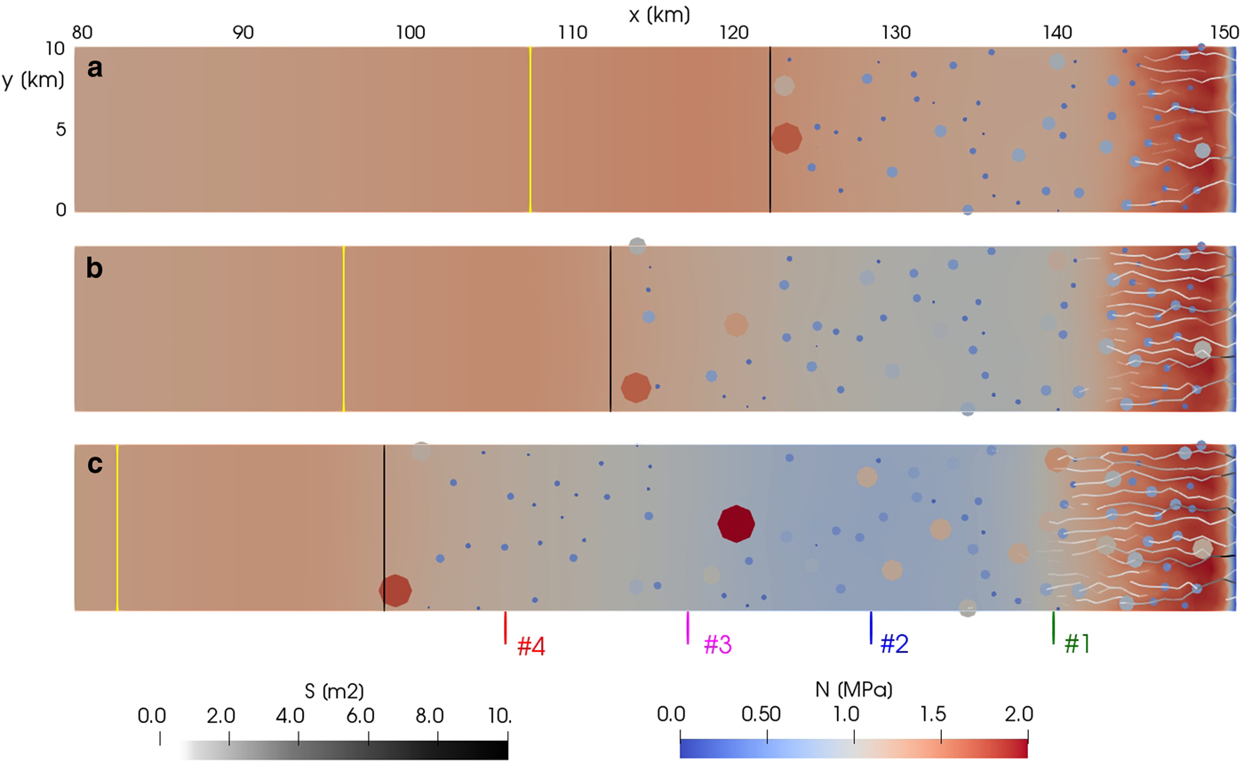
Fig. 4. Effective pressure N and channel cross-sectional area S at maximum channel extent during the melt season for (a) initial state, (b) year 20 and (c) year 40 of simulation STEP6. Circles indicate activated moulins with size proportional to the maximal input water for that year. The black line delimits the extent of the crevassed area and the yellow one the limit for surface melt. The positions of the four sites are indicated with the same colour code as in Figure 3. Note that only the last 70 km of the domain is represented.
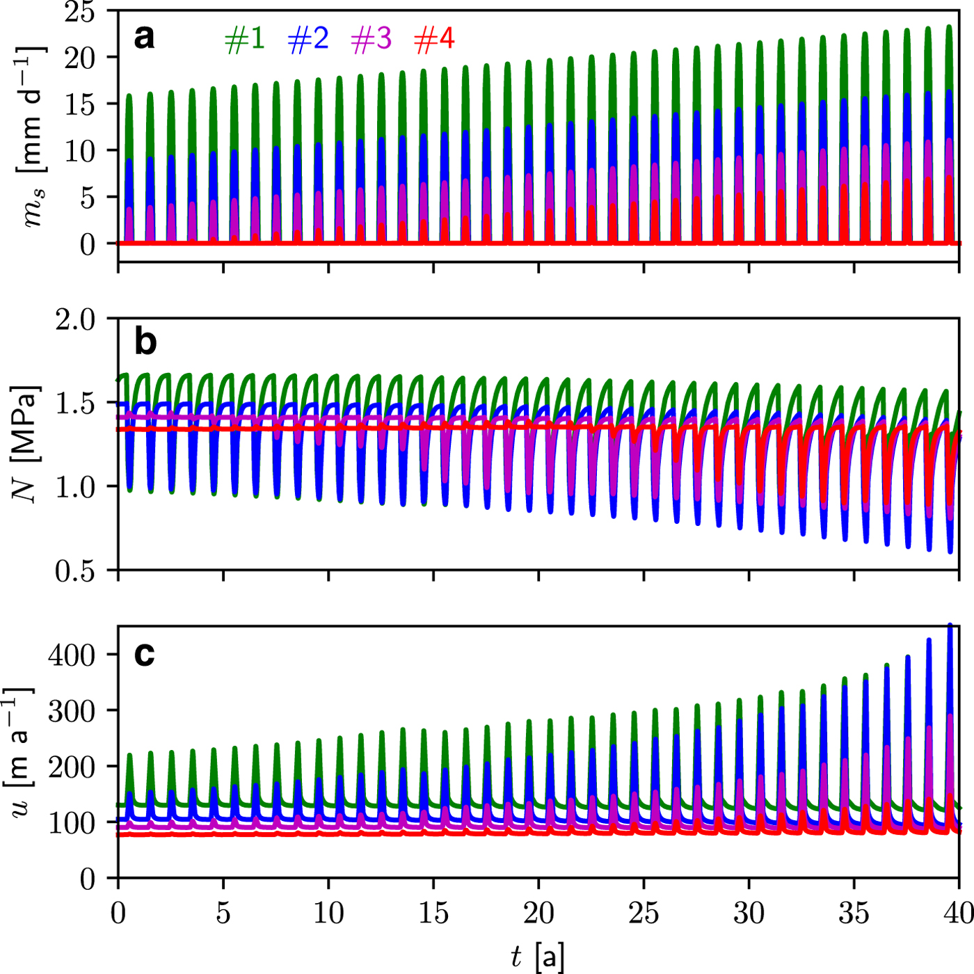
Fig. 5. STEP6: evolution over 40 years of laterally-averaged (a) surface melt m s, (b) effective pressure N and (c) surface velocity u at the four sites on the glacier. The location of the four sites is given in Figure 3 with the same colour convention.
Over the year, the spun-up solution indicates an increase of surface velocity that propagates upstream during the spring-summer months, in correlation with decreasing effective pressure. The crevassed area for the initial configuration extends over the first 28 km of the glacier up to an elevation of 1415 m (in between sites #2 and #3, see Figs 3a, 4a), inducing the activation of 60 moulins. Note that the seasonal variation of surface melt has an influence on ice flow over a larger area, up to at least site #3 (see the first year in Fig. 6c). This indicates that changes in basal conditions located in the crevassed area have an influence on the upstream ice velocity. As we will see below, this is the mechanism that can cause the upstream expansion of the crevassed area with increased surface run-off.
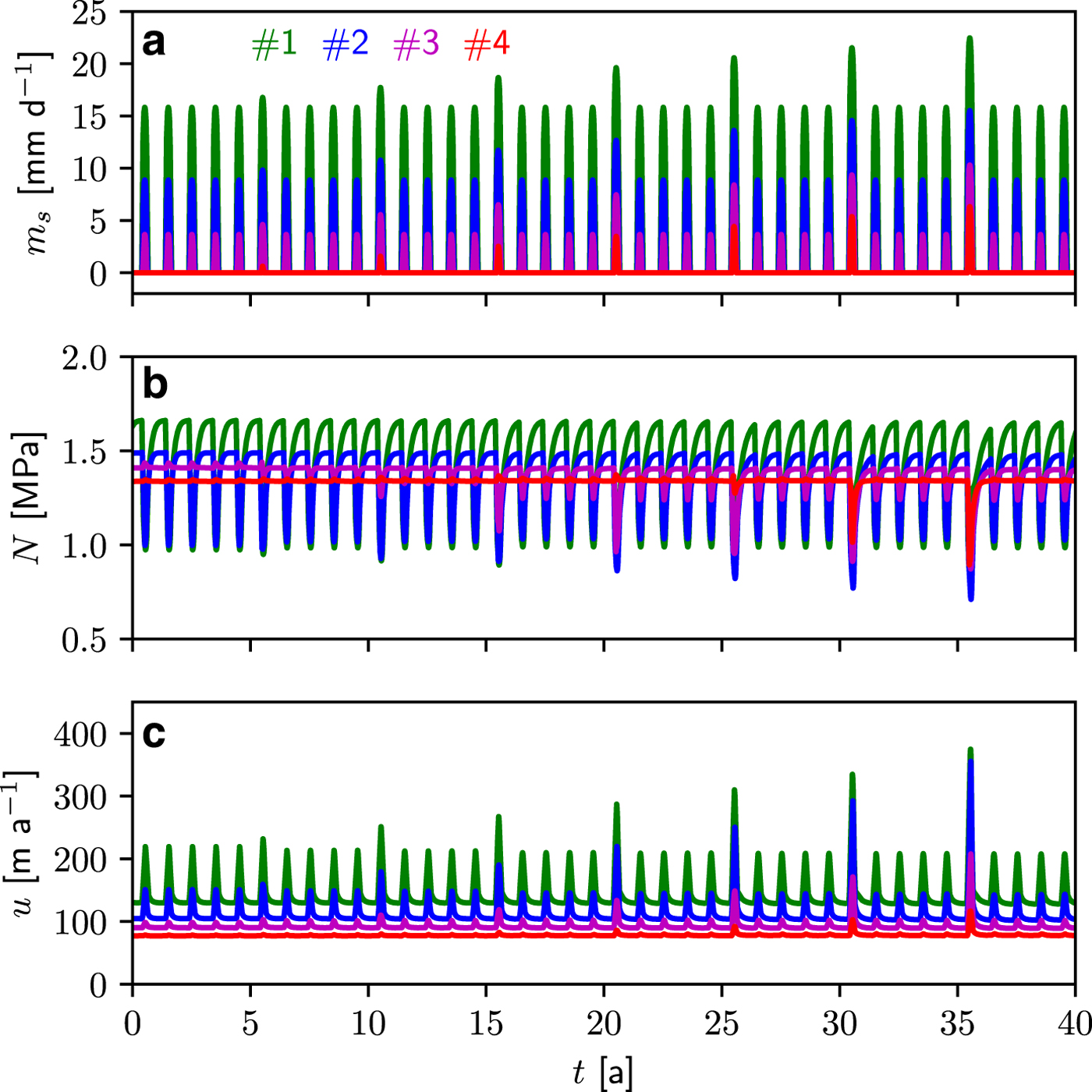
Fig. 6. Same as Figure 5 but for PEAK30.
As moulins are only activated in the crevassed area, no water from the surface reaches the bed upstream of the crevassed area. As a consequence, water input into a few moulins located just downstream of the limit of the crevassed area can be much larger than into the ones just below because they drain much larger area (see Fig. 4a).
3.2 Perturbation experiments
The surface melt m s(x, t) at the four sites is represented in Figure 5a for STEP6 and in Figure 6a for PEAK30. The corresponding annual surface mass balance at the same four sites is depicted in Figure 7c for STEP6 and in Figure 8c for PEAK30. For all other scenarios, the same information is provided in the corresponding figures in the supplementary material. The evolution over the 40 years of the laterally-averaged effective pressure and sliding velocity at the four sites is shown in panels b and c in Figure 5 for STEP6 and in Figure 6 for PEAK30. Figures 7, 8 show the evolution of the laterally and yearly-averaged (a) velocity relative to the initial state and (b) the rate of surface lowering for STEP6 and PEAK30 experiments, respectively.
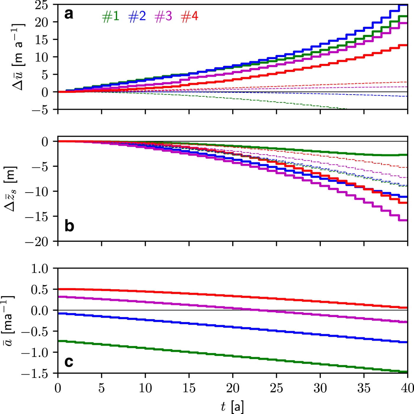
Fig. 7. STEP6 (thick, solid lines): evolution over 40 years at the four sites located in Figure 3 of the laterally-averaged mean annual change in (a) velocity  $\Delta \bar {u}$ and (b) surface elevation $\Delta \bar {z}_{{\rm s}}$ relative to the initial year-to-year steady-state configuration. The annual surface mass balance $\bar {a}$ in m ice eq. is depicted in (c). The thin, dashed lines represent the solution with a constant amount of input water Q s (equal to the first year of STEP6) into the moulins over the 40 years. This solution shows the effect of a decreasing surface mass balance alone without the coupling to sliding velocity. In panel (c), the changes in surface elevation are too small to distinguish the differences in surface mass balance.
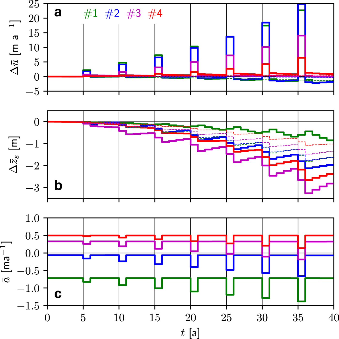

For the STEP6 experiment, the mean annual velocity is continuously increasing over the 40 years at the four sites but the increase is not directly related to the site location (Fig. 7a). Indeed, larger changes in velocity are obtained at site #2 than #1 after year 15, which presents similar changes than those at site #3. As a consequence, the velocity at site #2 becomes almost equal to the one at #1 at year 37. The smallest changes in velocity are observed at site #4. Over the 40 years, surface elevation changes least at site #1 (−3 m) and most at site #3 (−16 m), indicating two different type of balances depending on elevation (Fig. 7b). At low elevations, increased surface melt is partially offset by increased ice flux from upstream, resulting in relatively small changes in surface elevation. Indeed, at site #1, ice flux almost balances the doubling of the negative surface mass balance over the 40 years of simulation (from − 0.73 to − 1.47 m~a−1 ice eq.) and surface elevation even increases over the last few years. The same trend in surface changes is seen at site #2 which seems to also stabilize due to an increased flux from upstream (see also supplementary Figure S11 for STEP8 for which it is amplified). At higher elevations, surface changes are controlled by increasing surface melt which is not compensated by an increased ice flux. Indeed, basal velocities of these upper regions are not yet being affected by the increased surface melt. Surface elevation lowering is heterogeneously distributed which causes the lower parts of the glacier to flatten, consequently, the slope in an intermediate, upward-moving region steepens, but the upper parts, still unaffected by melt, remain unchanged. As will be discussed below, this region of increasing slopes is, however, not the primary source of control on crevasses opening and propagating upstream.
Figure 4 shows map views of the drainage system of three snapshots of the experiment STEP6 at the initial state, year 20 and year 40. The number of activated moulins progressively increases from 60 at the initial state to 93 after 40 years. The channelized system propagates upstream as melt increases over the years, but it does not reach further inland than approximately 15 km, certainly because the melt season is too short to allow the propagation of channels further inland. As a consequence water reaching the bed upstream of the channelized system will flow through an inefficient system, in which N decreases with discharge. Such results are in agreement with observations and previous modeling in Greenland (Meierbachtol and others, Reference Meierbachtol, Harper and Humphrey2013). This particular development of the sub-glacial hydrology system certainly explains the non-linear increase of ice velocity in response to an almost linear increase in the surface melt (Fig. 5a-c). Also in agreement with observations is that the limit of the crevassed area (black line, Fig 4) is always located at a much lower elevation than the limit of surface melt (yellow line).
For PEAK30, the year with the peak melt induces large increases in mean surface velocity (Fig. 8a), followed during the next 4 years by slightly lower velocities relative to initial state ( $\Delta \bar {u} < 0$) at sites #1 and #2 and slightly higher ones at the two higher elevation sites. As for STEP6, but occurring at year 25 instead of year 15, changes in velocity during the peak year at site #1 become larger than at site #2. In terms of surface lowering rate, two different responses are obtained depending on the site's elevation (Fig. 8b). For the three highest elevations, the peak melt year induces a high lowering rate. The surface elevation is still decreasing the year after the peak melt year but is then followed by 3 years of increasing surface elevation, that partially compensate the loss during the 2 previous years. Nevertheless, the general trend is a decrease of the surface elevation at these high altitudes. In terms of interannual variability, changes of surface elevation at site #1 are in opposite phase with the three other sites. At this low elevation site, which presents the highest melt rate, the general trend is closer to a steady surface elevation, indicating that ice flux from upstream more than compensates the increase in the surface melt. As for the STEP6 experiment, the smallest changes in surface elevation are observed at the lowest elevations (site #1).
Similar features in terms of velocity and surface elevation changes are obtained for the other STEP and PEAK experiments as shown in the Figs S2, S14 in the supplementary material.
To quantify the contribution to surface elevation changes by the decreasing surface mass balance alone, we set up a set of simulations in which the additional run-off due to increased melting is not routed through the subglacial drainage system, i.e. moulin input stays as in the first year and surface elevation changes are solely induced by the decreasing surface mass balance. Thus, ice dynamics can only evolve due to surface topography changes and not due to enhanced basal sliding. The results from these simulations (dashed lines in Figs 7, 8 and Figs S2, S14) show, as expected, changes in velocity that are much smaller than for the corresponding fully-coupled simulations and qualitatively different, with the lower two sites #1 and #2 displaying a slowdown instead of an acceleration. Contrary to the corresponding fully-coupled simulations, changes in surface elevation are roughly proportional to the increase in surface melt: the higher the elevation the lower the elevation decrease. Interestingly, the total volume change of the glacier after 40 years is increased in all cases by a few tens of percent when the coupling between basal hydrology and ice flow is accounted for. In other words, there is indeed a positive feedback such that the volume loss induced by increased surface melt is amplified by the influence of the increased run-off on ice dynamics (Zwally and others, Reference Zwally2002). Even if absolute elevation changes are much smaller in PEAK experiments than in STEP ones, the relative increase in volume loss due to the ice-dynamics feedback is almost identical for the same STEP and PEAK melt scenario, from 28% for STEP2 (23% for PEAK10) to 40% for STEP6 (41% for PEAK40).
Finally, Figure 9 depicts the temporal evolution of the maximum altitude of the crevassed area  $\tilde {z}_{{\rm s}}$ for each melt scenarios. For all the scenarios, $\tilde {z}_{{\rm s}}$ is increasing over the 40 years of the simulations with the consequence of activating new moulins at higher altitude with time. Depending on the scenarios, the initial elevation of 1415 m is increased by 75 m (PEAK10) to more than 400 m (STEP8) in 40 years. This corresponds to a horizontal displacement of the upper limit of the crevassed area of 5 km to more than 40 km in 40 years (See Figure S1 in supplementary material).
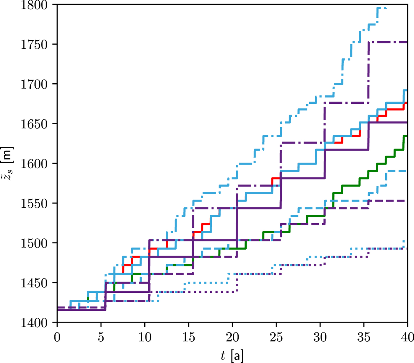
Fig. 9. Evolution with time of the maximum altitude of the crevassed area: in blue STEP2 (dotted), STEP4 (dashed), STEP6 (solid) and STEP8 (dash-dotted); and in purple PEAK10 (dotted), PEAK20 (dashed), PEAK30 (solid) and PEAK40 (dash-dotted). The solid red curve corresponds to the STEP6 forcing for a fixed upper free surface; the solid green line corresponds to the STEP6 forcing but without upstream activation of moulins (constant number of moulins over the 40 years).
Comparison of STEP and PEAK simulations shows that the crevassed area is mostly controlled by the amount of melt of a given year. Indeed, PEAK melt scenarios induce crevassed elevation changes every 5 years of the same magnitude as the cumulated STEP ones over 5 years. This indicates that extreme melt seasons, such as observed in 2012 for Greenland, could open crevasses at higher elevations. These crevasses are not necessarily large and might be difficult to detect from space, but could grow by hydrofracturing assuming they are not closed before enough meltwater reaches them. A crevasse-closure mechanism, not accounted for in our modelling, could thus reduce the impact of isolated warm years.
The comparison of experiments with and without evolving the free surface elevation for the STEP6 forcing (blue and red solid lines, respectively, in Fig. 9) shows almost no difference in  $\tilde {z}_{{\rm s}}$, thus the opening of crevasses is likely to be mostly controlled by increased gradients of horizontal velocity and not by the increased surface slope.
The last experiment assuming the STEP6 forcing is performed without evolving the number of moulins activated. In that case (green solid line in Fig. 9), the crevassed area extends much more slowly upstream, especially in the first two decades. However, even without the progressive activation of new moulins, differences in the basal condition in the upper part of the glacier, not influenced by hydrology and in the lower part, receiving more and more water each year, are such that tensile strain rates large enough to open new crevasses propagate far upstream of the highest activated moulins. This gives confidence that, even with a long multi-year or decade delay between the potential opening of new crevasses and the effective activation of moulins, an increase in the amount of water at the base of the lower part of a glacier could create an internal state of stress allowing the upstream propagation of new crevasses.
4. DISCUSSION
Our model results suggest that the crevassed areas of the land-terminating outlet glaciers of Greenland will move further inland as climate change increases the area affected by surface melt, with the consequence that surface meltwater can access the bed further inland. The effect on the effective pressure of increased subglacial discharge can either be positive or negative, depending on whether the system is in an efficient (channelized) or inefficient (distributed) configuration. Our results show that with increased surface melt the drainage system will remain inefficient for the most part and that the area occupied by channels increases much less than the area of the bed accessed by surface water (Fig. 4). Note that this discrepancy is likely to increase even more in the future as the channelized area will not grow much more (Meierbachtol and others, Reference Meierbachtol, Harper and Humphrey2013) but the area subjected to surface melt likely will. The increased discharge in the inefficient system lowers the effective pressures and the coupled ice flow model then indeed produces much-enhanced flow velocities (e.g. Fig. 7a).
As discussed in the Introduction, observations in Greenland show that an increased melt rate can either cause a mean annual ice flow speed-up (e.g. Zwally and others, Reference Zwally2002; Shepherd and others, Reference Shepherd2009; Bartholomew and others, Reference Bartholomew2010; Doyle and others, Reference Doyle2014) or a slow-down (Tedstone and others, Reference Tedstone2013, Reference Tedstone2015). The PEAK simulations proposed in this study indicate an opposite response in terms of mean annual velocity depending on the elevation (Fig. 8). Indeed, velocities at low elevations increase in the year after a peak melt year, but it is the opposite at higher elevations. In line with the conclusion of de Fleurian and others (Reference de Fleurian2016), our results using a synthetical geometry might explain why the various field observations found opposite effects after a year of enhanced surface melt.
Our findings contrast with the conclusions drawn by the observation-based study by Poinar and others (Reference Poinar2015), which states that crevassing will not extend further inland, but are in line with the recent observations of Yang and Smith (Reference Yang and Smith2016) that crevasses can open at higher elevation than previously thought. Hoffman and others (Reference Hoffman2018) and Christoffersen and others (Reference Christoffersen2018) suggest that the drainage of supraglacial lakes is responsible for inland migration of crevassing, however, our results suggest that the migration can also happen without those drainages.
The comparison of simulations accounting for the full coupling of hydrology and ice flow with the corresponding simulations accounting only for surface lowering indicates a positive feedback which increases the volume changes by a few tens of percent after 40 years. As the velocity between these two solutions are diverging (see e.g. Fig. 7a), it is likely that the differences in volume loss will be much larger over longer time periods. The excess in volume loss when accounting for the coupling is mostly explained by the increased ice flow occurring at high elevations which induces surface elevation decreases much higher than those obtained only by surface melt.
Finally, there are missing processes in our modeling approach that might affect conclusions drawn from our results. By assuming that moulins open instantaneously as long as they are located in the crevassed area, the run-off is certainly routed down to the bed at higher elevations more rapidly than in reality. Also, would a small crevasse survive one winter if hydrofracturing has not been at play? By not accounting for crevasse closing, we might overestimate the rate at which crevasses propagate upstream. On the other hand, our model does not account for supraglacial lakes and their drainage, which has been shown to be a primary control of moulin formation (Christoffersen and others, Reference Christoffersen2018; Hoffman and others, Reference Hoffman2018). Another missing mechanism is the retention of surface meltwater within the firn, which could delay the water availability at higher elevation by storing this water. Indeed, as shown by Steger and others (Reference Steger2017), as much as 45% of the meltwater produced at high elevation could be stored in the firn either by capillary forces or by refreezing. Also, changes in ice temperature are not accounted for in our model. Water might reach bed areas with a currently cold base, in which case it would probably refreeze. On the other hand, increased basal sliding will certainly progressively move the limit between temperate and cold base upstream, due to increased frictional heat. All the above-mentioned model limitations could only delay the propagation of crevasses upstream and, therefore, influence the vicinity at which water is able to reach the bed at higher elevations, but would not counteract totally this upstream propagation (green solid line in Fig. 9). Therefore, the fact that under increasing run-off the crevassed area is likely to reach higher elevations is a robust feature of our model results.
5. CONCLUSION
We have developed a model framework that accounts for a number of processes at play for land-terminating glaciers in Greenland. The model couples ice flow, surface evolution, crevasses opening and the different components of the hydrology system. All these equations have been implemented in the open-source finite-element ice flow model Elmer/Ice. Synthetical experiments for various surface melt increases have been conducted with the objective of simulating the upstream propagation of the crevassed area of the glacier.
In terms of ice volume loss, accounting for the coupling between ice flow and basal hydrology results in a net volume loss significantly larger (from 23% to 41% after 40 years depending on the melt scenario) than the one solely induced by the decrease in surface mass balance. As land-terminating glaciers represent up to 10% of the total ice volume above floatation of the Greenland ice sheet (Mouginot, personal communication), this dynamical component might contribute to the global mass loss more than previously thought. Dedicated coupled hydrology-ice flow studies on different Greenlandic land-terminating glaciers are needed in order to confirm the significance of this contribution to the global budget of the ice sheet.
As the main result of this work, we have shown that contrary to the conclusions drawn by Poinar and others (Reference Poinar2015) from observations of the current state of the Greenland ice sheet surface, the inland migration of melt is likely to extend the crevassed area up-glacier in the near future. This upstream migration of crevasses will allow new meltwater to reach the bed farther inland and hence ice flow to be influenced by basal hydrology over larger areas. As a consequence, the mean annual velocity at these higher elevations will increase and more ice will be transported to the frontal regions where the surface melt is highest, therefore, increasing the total mass loss of these land-terminating glaciers.
SUPPLEMENTARY MATERIAL
The supplementary material for this article can be found at https://doi.org/10.1017/jog.2018.59
ACKNOWLEDGMENTS
We thank G. Durand for discussions that initiated the setup design of these experiments and X. Fettweis for providing surface run-off from the MAR model using ERA-Interim reanalysis from 1979-2014. We thank the editor, D. Shugar, the chief editor, G. Cogley, as well as the two anonymous referees for their insightful and helpful comments.
APPENDIX
In this Appendix are described some technical points regarding the implementation of the GlaDS model in Elmer/Ice. Following Werder and others (Reference Werder, Hewitt, Schoof and Flowers2013), the evolution in space and time of the hydraulic potential ϕ is given by the following weak formulation of Eqns (13), (14) and (10):
 $$\eqalign{& \sum\limits_i {\int_{\Omega _i} {\left[ {\theta \displaystyle{{e_{\rm v}} \over {\rho _{\rm w}g}}\displaystyle{{\partial \phi } \over {\partial t}} - \nabla \theta \cdot {\bi q} + \theta \left( {w_{\rm s} - m_{\rm b} - v_{\rm s}} \right)} \right]} } \,{\rm d}\Omega \cr & + \sum\limits_j {\int_{\Gamma _j} {\left[ { - \displaystyle{{\partial \theta } \over {\partial {\rm s}}}Q + \theta \left( {\displaystyle{{\Xi - \Pi } \over L}\left( {\displaystyle{1 \over {\rho _i}} - \displaystyle{1 \over {\rho _{\rm w}}}} \right) - v_{\rm c}} \right)} \right]} } \,{\rm d}\Gamma \cr & + \int_{\partial \Omega _N} \theta q_N{\rm d}\Gamma - \sum\limits_k \theta \left( { - \displaystyle{{A_{\rm m}^k } \over {\rho _{\rm w}g}}\displaystyle{\partial \phi \over {\partial t}} + Q_{\rm s}^k } \right) = 0,}$$
where θ is a test function, Ωi the sheet subdomains, Γj the channel segments and ∂ΩN the boundary on which the discharge q N is imposed. Note that, as explained in Werder and others (Reference Werder, Hewitt, Schoof and Flowers2013), for each edge element the water exchange between sheet and channel term m c in (14) cancels with the boundary flux term from the two adjacent sheet elements. More details regarding the derivation of the weak formulation can be found in Werder and others (Reference Werder, Hewitt, Schoof and Flowers2013).
Equation (A1) using (17)–(23) is first solved to determine the hydraulic potential ϕ for given h and S. Non-linearity in this equation arises because of the water discharges q and Q and the closing rates v s(h, N) and v c(S, N). Defining γ = |ϕ 0 − ϕ|n−1(ϕ 0 − ϕ) = |N|n−1N and  $\tilde {A} = 2 A/n^n$, the term v s(h, N) at iteration p+1 of the non-linear loop is evaluated using a Newton linearization as
 $$\eqalign{\tilde Ah\gamma _{\,p + 1} & = \tilde Ah\left[ {\gamma _{\rm p} + (\phi _{\,p + 1} - \phi _{\rm p}) {\left. \displaystyle{{\partial \gamma } \over {\partial \phi }} \right \vert}_{\phi _{\rm p}}} \right] \cr & = \tilde Ah\left[ {\gamma _{\rm p} - n(\phi _{{\rm p} + 1} - \phi _{\rm p}) \vert \phi _0 - \phi _{\rm p} \vert ^{n - 1}} \right] \cr & = \tilde Ah \vert \phi _0 - \phi _{\rm p} \vert ^{n - 1}(\phi _0 + (n - 1)\phi _{\rm p} - n\phi _{{\rm p} + 1})}$$
The term  $- n \tilde {A} h \vert \phi _0 - \phi _{{\rm p}} \vert ^{n-1}$ is added to the diagonal terms of the stiffness matrix whereas the second part of v s(h, N), $\tilde {A} h \vert \phi _0 - \phi _{{\rm p}} \vert ^{n-1} (\phi _0 + (n-1)\phi _{{\rm p}})$ is put in the second member. Same is done for the channel closure rate v c.
As depicted in Figure 2, during a time step, Eqns (A1), (15) and (16) are solved iteratively until a convergence is obtained, which is assumed to be the case if the relative difference between two coupled iterations of the norm of the solution for the hydraulic potential ϕ is lower than 10−3.
Equations (15) and (16) are local equations which depend only on the time derivative of the variables h and S and can therefore, be solved directly at each node and edge, respectively, of the domain. Because of the flux Q entering (16), the equation is non linear and needs to be iterated. Equation (15) is integrated in time using a fully implicit method whereas for (16) a Crank--Nicolson scheme is adopted.


 Open access