


1. Introduction
Ice core studies with high sampling-resolution chemical and isotopic analyses are essential to ascertain information important in various aspects of glaciology. The annual layer thickness in ice cores collected at low accumulation sites from Antarctica, however, can be as small as ~1 cm or smaller at deeper depths. For example, at a depth of about 2100 m in the DF2 ice core (Motoyama, Reference Motoyama2007; Kawamura and others, Reference Kawamura2017; Motoyama and others, Reference Motoyama2021) drilled at Dome Fuji Station (77° 19′ 01″ S, 39°42′ 12″ E) in East Antarctica, the estimated age is about 200 000 years BP (before the present) and the annual layer thickness is estimated to be about 0.5 cm. When we try to extract various types of information from past environments in such deep ice cores to elucidate continuous, long-term, annually resolved profiles, we are facing a boundary of sampling technique and apparently need a new sampling method.
So far, to sample and analyze ice cores continuously with relatively high resolution, the heater-melting continuous flow analysis (CFA) method has been widely used (Röthlisberger and others, Reference Röthlisberger2000; McConnell and others, Reference McConnell, Lamorey, Lambert and Taylor2002; Traversi and others, Reference Traversi2002; Kaufmann PR and others, Reference Kaufmann2008; Bigler and others, Reference Bigler2011; Emanuelsson and others, Reference Emanuelsson, Baisden, Bertler, Keller and Gkinis2015; Severi and others, Reference Severi, Becagli, Traversi and Udisti2015; Dallmayr and others, Reference Dallmayr2016; Jones and others, Reference Jones2017; Grieman and others, Reference Grieman2022). The depth resolution of the CFA systems overall is usually ~10 mm or more, although a resolution of a few millimeters has been achieved for measurements of Na+, NH4+, and dust particles (Bigler and others, Reference Bigler2011).
Laser ablation inductively coupled with plasma mass spectrometry (LA-ICP-MS) is another widely used method to sample and analyze ice cores (Reinhardt and others, Reference Reinhardt2001; Müller and others, Reference Müller, Shelley and Rasmussenc2011; Sneed and others, Reference Sneed2015; Della Lunga and others, Reference Della Lunga, Müller, Rasmussen, Svensson and Vallelonga2017; Bohleber and others, Reference Bohleber, Roman, Šala and Barbante2020). Sneed and others (Reference Sneed2015) reported achievement of a sub-millimeter depth resolution. The LA-ICP-MS method, however, is probably not well suited for isotopic analysis of water because laser ablation is a violent process and complex secondary processes can occur due to the very high temperature rise in the laser-irradiated part. We, therefore, developed a new device, a novel laser melting sampler (LMS) for ice cores, specially designed for measuring the stable water isotope ratios, δ18O and δD, to enable us to attain the necessary high-depth resolution without significant isotopic fractionation.
The LMS system is outlined as follows: in a low-temperature room, a sectional portion of an ice core segment is laid on a horizontally sliding stage. A 2 mm diameter movable evacuation nozzle, that holds an optical fiber inside, intrudes into the ice, melting it cylindrically by laser irradiation and transferring the meltwater simultaneously into a collection buffer by means of a peristaltic tube pump. To avoid isotopic fractionation through vaporization, the laser power is adjusted to keep the temperature of the meltwater well below its boiling point. The meltwater is collected repeatedly until the amount necessary for the planned analysis has been accumulated, and the collected water is then pumped into a vial for the offline analyzer. By a combination of vertical and horizontal movements, the ice core segment is sampled discretely. The depth resolution normally attained is as small as 3 mm, which has been difficult to achieve with conventional systems.
In this paper, we will describe the details of the LMS. It will be shown through the performance tests that a 3 mm depth resolution sampling was achieved with the LMS, and the subsequent measurement of the water isotope ratios, δ18O and δD, will then be demonstrated on a portion of a Dome Fuji shallow ice core recovered from Antarctica.
2. The LMS for ice cores
2.1 Overview of the LMS system
The LMS (Fig. 1) consists of four major components: (1) sampling unit, (2) sliding stage, (3) stainless steel vials in two sets of vial trays, and (4) conveyor system. The LMS is placed in a low-temperature room kept at −20°C. The computer control system of the LMS and a continuous-wave operated Er-doped fiber laser (CEFL-TERA, Keopsys Inc.) for melting ice are placed in an ambient temperature room outside the low-temperature room.

Figure 1. (a) Schematic drawing of the LMS. (b) Photograph inside the low-temperature room. A CMOS (complementary metal oxide semiconductor) camera is mounted on the sampling unit to monitor the melted state of the ice core under laser irradiation.
The sampling unit of the LMS, the details of which are described in Section 2.2, is equipped with a specially designed nozzle made of silver, into which the optical fiber is inserted, and the meltwater produced by laser irradiation is removed by a peristaltic tube pump. Once collected in a sampling buffer tube inside the sampling unit, the meltwater is finally pumped to a stainless steel vial waiting outside. The position of the sampling unit is fixed in the z-direction in Figure 1 (the depth direction of the ice core), and the sampling unit is moved in the x- and y-directions (Fig. 1) by a cross-ladder elevation mechanism and a ball-screw linear actuator driven by a stepping motor, respectively. The positioning reproducibility is better than ±0.05 mm with rotary encoders. We can add another identical sampling unit for high throughput sampling, e.g. as illustrated in Figure 1a.
A 50 cm-long portion of an ice core segment is laid horizontally, an orientation favorable for sampling even fragile firn cores, on the sliding stage. The position of the ice core is shifted horizontally (in the z-direction) by a ball-screw linear actuator equipped with a rotary encoder. By combining the movements of the sampling unit and sliding stage we can sample the ice core selectively at whatever positions may be required.
The vial tray stores 54 (6 × 9) vials and the conveyor system transports the vials one by one to the meltwater drain position underneath the outlet of the sampling unit, returning them to the tray after the vial has been filled with meltwater. The target volume of the meltwater stored in a vial is adjustable, as mentioned in Section 2.2, and is typically 1.5 mL. At present, the vial trays are collected and set in position for the analyzers by hand.
2.2 Sampling unit and operation
The components of the sampling unit (10 cm wide × 25 cm long × 13 cm high) are shown schematically in Figure 2 and in the photograph of the interior viewed from above in Figure 3. The interior of the sampling unit is kept warm, at above 0°C, by resistive sheet heaters.

Figure 2. Schematic development diagram detailing the components of the sampling unit.

Figure 3. A photograph of the top view of the interior of the sampling unit.
The laser beam is transferred through a silica core multimode optical fiber (core/clad diameter = 200/220 μm) to the sampling unit. The laser wavelength is 1.55 μm (near infrared), which does not cause photolysis in the samples, and the maximum output power is 10 W. The 1.55 μm wavelength takes advantage of the strong absorption bands of ice and water from 1.4 to 1.6 μm (Warren and Brandt, Reference Warren and Brandt2008; Kedenburg and others, Reference Kedenburg, Vieweg, Gissibl and Giessen2012). A further merit of employing this wavelength is that suitable optical fibers are available commercially.
The 60 mm-long nozzle (Figs. 2 and 3) is made of commercially available pure Ag999 tubing (2 mm outer diameter and 1 mm inner diameter) and is kept warm, at well over 0°C, in the −20°C environment by the conduction of heat generated by the resistive heater block at the rear end of the nozzle (Figs. 2 and 3). The tip of the nozzle (Fig. 4) is plugged by a cylinder of polyether ether ketone (PEEK) resin, 4 mm long, at the center of which a 0.5–0.35 mm diameter stainless steel capillary is inserted to hold the optical fiber in place with an acrylate coating (Coating diameter = 0.32 mm). The meltwater is siphoned through a small opening at the bottom of the PEEK plug (~0.2 mm2).

Figure 4. Schematic diagram of the Ag999 nozzle tip for laser melting/sampling.
At the beginning of sample collection, the tip of the nozzle is located at a point a few mm away from the side of the ice core. As the nozzle advances in the y-direction (see Fig. 1), the laser beam delivered through the optical fiber irradiates the ice core to melt it; the meltwater is simultaneously vacuumed through the nozzle and transferred through a perfluoroalkoxy alkane (PFA) polymer tube into a PFA sampling buffer (Figs. 2 and 3) which is depressurized by a peristaltic tube pump. Conventionally, this pump is utilized to move liquid forward or backward in a tube. On the other hand, in the LMS, this pump is utilized to evacuate air in the buffer to induce airflow in the transfer tube. As a result, the meltwater drops are intermittently transferred with this airflow at an air pressure in the tube that is close to 1 atm.
When the nozzle reaches the pre-specified intrusion depth, the nozzle is withdrawn to the start position. If more meltwater is needed, e.g. in a high-resolution sampling mode, the nozzle is shifted vertically and the sample collection is repeated. A non-contact water level sensor attached to the sampling buffer interrupts sampling when the target volume of sample water (adjustable: ~0.65 to ~2.5 mL) has been collected in the sampling buffer. Then, the sampling unit is pulled back from the ice and both the laser beam and the tube pump are deactivated. Immediately, the three-way solenoid valve connected to the sampling buffer is switched and, by reversing the tube pump, the meltwater stored in the sampling buffer is pumped into a vial waiting underneath the drain outlet of the sampling unit.
3. Performance tests of LMS
3.1 Sampling parameters and discreteness
First, the switch-on timing of the laser beam had to be determined and set to prevent the nozzle tip from colliding with the frozen ice-core surface. Then, to achieve smooth and efficient sampling, we needed to optimize (1) the laser power, (2) the intrusion speed of the nozzle into the melting ice core, and (3) the rate at which the meltwater is vacuumed up.
The higher the laser power, the faster the melting rate, but the meltwater must not boil. We determined an adequate laser power to be ~2.0 W in a −20°C environment, under which conditions the meltwater never boils near the optical fiber tip. The meltwater had to be vacuumed up as quickly as possible to avoid overheating by the laser but, on the other hand, the meltwater would not have been vacuumed up efficiently had the pumping speed been too fast. As a result of trials using blocks (density ~0.93 g cm−3) of frozen ultrapure water (Milli-Q water) at −20°C and a laser power of ~2.0 W, we determined that a tube pump speed of ~5.5 mL min−1 was appropriate. Finally, the optimal nozzle intrusion speed to maintain a cylindrical melting region of ~3 mm in diameter was determined to be ~0.52 mm s−1.
Considering the amount of meltwater collected, the time required for collection, and the pumping speed, we found that the meltwater was vacuumed up intermittently although the tube pump was operated continuously: for ~97% of the pumping time, only air was vacuumed up.
Under the above conditions, by observing the irradiation point with the CMOS (complementary metal oxide semiconductor) camera (Fig. 1b), we ascertained that there were no signs of boiling during sampling. This result was consistent with the following rough estimation of the meltwater temperature ΔT on the assumption that the laser power of 2 W was balanced with the heat ΔH needed to melt the ice and warm up the meltwater. ΔH is estimated as:

where C i (2.1 J g−1K−1) and C w (4.2 J g−1K−1) are the specific heats of ice and water, respectively, and H m (336 J g−1) is the fusion heat of ice. The quantity M w in Eqn (1), the meltwater weight per unit time is estimated to be 0.0034 g s−1 using our values of melting diameter and intrusion speed. From the balance of input power with the heat used to warm and melt the ice, the meltwater temperature ΔT is estimated to be 49°C. Given that we are neglecting heat dissipation from the melting region, the actual value of ΔT should be less.
Figure 5a shows a series of sampling holes in a block of Milli-Q ice, illustrating the discreteness of sampling that is possible with the LMS. The holes represent 10 meltwater samples of ~0.7 mL each, separated horizontally by 3 mm. In this demonstration, the laser power was set at ~1.8 W, the intrusion speed was 0.52 mm s−1, and the pumping speed was 5.5 mL min−1. In Figure 5a, each track of the sampling holes is seen to be well separated. This shows that samplings can be very close together without any intermixing with neighboring samples, thus successfully attaining a depth resolution of ~3 mm. In Figure 5b, we show a photograph taken at the beginning of the sampling when the nozzle had intruded 7 mm into the side of another block of Milli-Q ice. In this demonstration, the laser power was set at ~1.3 W, the intrusion speed was 0.20 mm s−1, and the pumping speed was 10 mL min−1. It is clearly shown in Figure 5b that the ice is melted by laser irradiation.
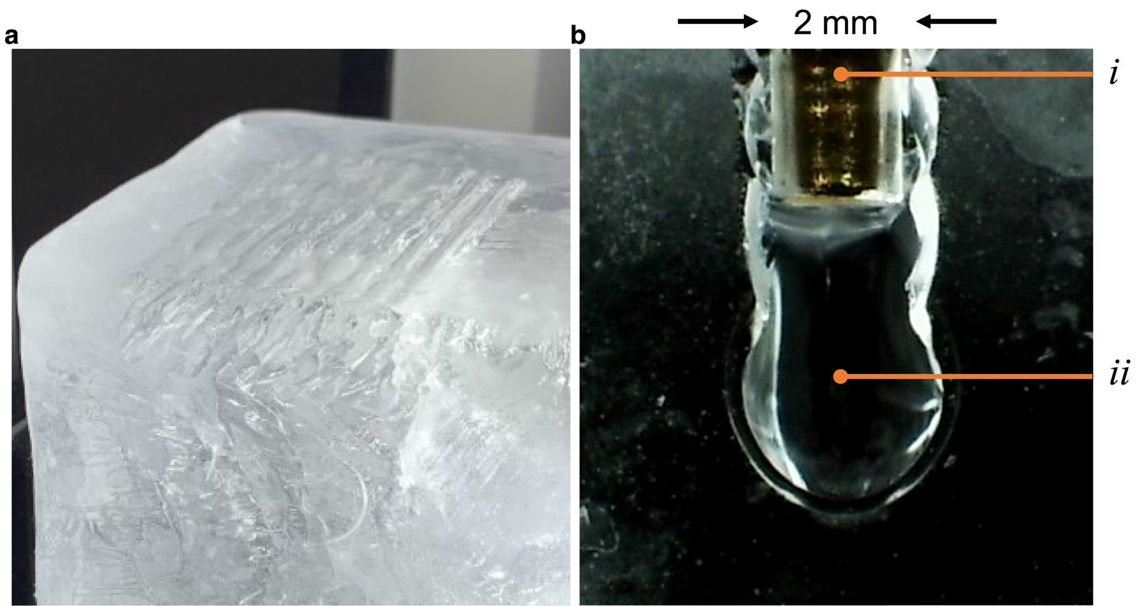
Figure 5. (a) A photograph showing multiple cylindrical holes 3 mm apart made by the LMS in a Milli-Q ice block. (b) A photograph of the first intrusion of the sampling nozzle into another Milli-Q ice block, taken by the CMOS camera mounted on the sampling unit: (i) 2 mm ϕ Ag nozzle, (ii) a meltwater zone.
3.2 Stability test for long series of samplings
To check the operational stability of the LMS in the −20°C environment, we performed a long series of sampling tests in which 100 vials were filled with a minimal volume (~0.65 mL) of meltwater. In this test, the laser power was set at ~1.9 W, the nozzle intrusion speed was 0.52 mm s−1, the pumping speed 5.5 mL min−1, and the horizontal and vertical pitch 2.5 mm. This test took 8 h 47 min to complete in the −20°C environment, and yielded, without issues, an average sampling time per vial of 5.3 min: 4.0 min to collect the water sample and 1.3 min to cycle the laser power, evacuate the meltwater sample, and move the sampling unit from and to the starting position for sampling.
In this stability test with a series of 100 vials, the amount of meltwater collected was 0.65 ± 0.02 mL per vial. Thus, the time required to sample the preferred volume of 1.5 mL would be ~11 min. This time is considerably shorter than the time required to analyze the oxygen and hydrogen isotopic composition of a sample in our operating protocol using a Los Gatos liquid water isotope analyzer (LWIA, model 912-0008-000, Los Gatos Research, Inc.). It is, therefore, concluded that the sampling rate will not be a bottleneck during offline isotopic analyses.
4. Application of LMS to a Dome Fuji shallow ice core
We applied the LMS to sampling a 50 cm-long segment of a Dome Fuji shallow ice core (DFS10) drilled in East Antarctica by the 51st Japanese Antarctic Research Expedition in 2010. The segment corresponds to ~91.6 m in depth and is thin and rectangular with a length and a height of 24 mm and 58 mm, respectively (Fig. 6). The segment density was ~0.76 g cm−3. In this first automatic sampling by the LMS of an Antarctic ice core, the sampling was undertaken over a depth span of 15 cm with a sampling pitch of 3 mm: 51 samples of meltwater at 3 mm depth resolution, as shown in Figure 6, were successfully collected in 51 vials. In this experiment, the laser power was set at ~1.9 W, the nozzle intrusion speed was 0.52 mm s−1, and the pumping speed was 5.5 mL min−1. The intrusion length of the sampling nozzle was set at 19.5 mm and, on average, 1.84 mL of meltwater per vial was collected. This implies that almost 100% of the meltwater was collected for the subsequent water isotope analyses.

Figure 6. A photograph showing discrete cylindrical holes after sampling (51 vials) a 15 cm-long section of a Dome Fuji shallow ice core (DFS10) drilled in East Antarctica. The sampling pitch in the depth direction of the ice core (the z-direction in Fig. 1) was set at 3 mm; the sampling pitch in the sectional direction (vertical direction in the photograph) was set at 2.5 mm. This photograph was taken from the direction of the sampling unit (see Fig. 1b).
The measurements on δ18O and δD were undertaken using the LWIA instrument mentioned in Section 3.2. The typical instrumental precision of the model used in this study is given as ±0.16‰ for δ18O and ±0.88‰ for δD for one-run measurement. Using these values, the instrumental precision for the deuterium excess (denoted by d being defined as d = δD – 8 × δ18O [Dansgaard, Reference Dansgaard1964]) is derived as ±1.55‰. The d value is a second-order isotopic parameter and reflects kinetic fractionation effects during evaporation and condensation on a water surface (Merlivat and Jouzel, Reference Merlivat and Jouzel1979). In our case, the d value can be used as a marker for the fractionation caused by evaporation or sublimation processes that may occur in the LMS system. We further investigate the standard deviation values (1σ) for the primary standard solution (SLAP2) to be tested as a sample from ten-runs measurements performed on different days using the same calibration standards. The results were about ±0.31‰ for δ18O and ±1.55‰ for δD. Using these values, the corresponding uncertainty of the d value is derived as ±2.94‰. These 1σ uncertainties can be regarded as typical analytical uncertainties concerning measurement accuracy and so are suitable for analyzing the data obtained from experiments performed on different days.
The water isotope compositions of δ18O, δD, and the d values with sampling at 3 mm pitch are shown in Figures 7a–c for the deeper half of the 7.5 cm span from the depth of 91.575 m of the DFS10 core. As the reference of the 3 mm pitch data, we also show in Figures 7a–c our results for the δ18O, δD, and d values for segments divided by hand with 2.5 cm depth resolution. Overall, we see that the 3 mm pitch LMS isotopic values are reasonably consistent with the 2.5 cm reference values obtained with hand segmentation. As shown in Figure 7c, the d data, the direct marker for isotopic fractionation that may occur in the LMS system, stay rather constant, and close to the 2.5 cm depth resolution results obtained by hand segmentation. We found in Figure 7c that the d values did not always show discrepancies in the same orientations relative to the 2.5 cm hand-cut reference values as were observed in δ18O and δD. These discrepancies indicate that no significant isotopic fractionation occurred when using the LMS system since it is natural to expect that the orientations of deviations caused by isotopic fractionation in the LMS would always exhibit the same orientations as the larger (heavier) isotopic values.

Figure 7. (a) The depth profiles of δ18O in the DFS10 shallow ice core obtained by the LMS at 3 mm pitch depth resolution (filled circles) and by hand segmentation at a 2.5 cm depth resolution (solid line) for comparison. (b) The same as (a) but for δD. (c) The same as (a) but for the deuterium excess (denoted by d). The selected depth range, from 91.575 to 91.650 m, corresponds to the deeper half of the sampling span of the DFS10 ice core shown in Figure 6.
The numerical data in Figure 7 are presented in Table 1 to show the values for 2.5 cm segments with hand segmentation (abbreviated as ‘Hand’ hereafter), the average values of the 3 mm pitch analytical results using the LMS within the depth span of each 2.5 cm segment (‘LMS’), the LMS − Hand differences for each 2.5 cm segment, and the standard deviations of the LMS measurements for each 2.5 cm segment.
Table 1. The δ18O, δD, and d values for 2.5 cm segments with hand segmentation (‘Hand’), the averages of the 3 mm pitch LMS data for δ18O, δD, and d within the depth span of each 2.5 cm segment (‘LMS’), the LMS − Hand differences, and the standard deviations of the 3 mm LMS sampling. Note that, in averaging, the 3 mm pitch data at 91.635 m are included in the segments of both 215-11 and 215-12

In Table 1, the LMS − Hand differences could have reflected the influence of laser irradiation and so warranted investigation. Considering that both the LMS sampled data and the hand-cut data were subject to the above-mentioned typical analytical uncertainties concerning measurement accuracy, the error propagation gives the 1σ analytical uncertainties for the LMS − Hand differences as being looser by a factor of √2: the uncertainties are then given as ±0.44‰ for δ18O, ±2.20‰ for δD, and ±4.16‰ for the d value. We thus confirm that the LMS − Hand differences given in Table 1 are almost within the 1σ analytical uncertainties. Only the difference of δD for Segment 215-12 is outside the 1σ boundary but here, just one of four data points is outside the 1σ boundary. This is statistically reasonable because the probability of a data point being within the 1σ boundary is about 0.68. We note that all four differences for the d value in Table 1 are within the 1σ boundary. It is thus concluded that the LMS − Hand differences are consistent with the analytical uncertainties for water isotope analyses of δ18O, δD, and d.
We also performed confirmatory tests to check the equivalence of the LMS data and hand-cut data. Since the pairs of hand segmentation data and the average values of the 3 mm pitch LMS data for each corresponding 2.5 cm segment, presented in Table 1, are directly comparable quantities that are suitable for investigation of the influence of laser irradiation, we performed t tests on these pairs. The results were p = 0.92 (t = 0.11) for δ18O, p = 0.36 (t = 1.09) for δD, and p = 0.62 (t = 0.55) for d, when the significance level was set to the usually used 0.05. Consequently, we can expect that there are no significant differences between the two data sets.
Unfortunately, the samples of the shallower half of the 7.5 cm sampling span were lost due to experimental contamination. We would emphasize, however, that this does not diminish the importance of the success of the first 3 mm pitch sampling by the LMS as applied to the section of the Antarctic ice core shown in Figure 6: this has opened up new possibilities for undertaking analyses of stable water isotopes at sub-centimeter depth resolution which we were hitherto incapable of doing.
We conclude from the examinations addressed above that our LMS does not cause significant isotopic fractionation: even if slight fractionation occurs during LMS sampling, it is at a low level compared with the fluctuations due to the measurement uncertainties in stable water isotope analyses of δ18O, δD, and d.
5. Conclusion and perspective
We have successfully developed a novel LMS to analyze the stable water isotope ratios in ice cores at sub-centimeter depth resolutions without significant isotopic fractionation. We have applied the LMS to ice blocks of frozen ultrapure water with a density of 0.93 g cm−3 and the segment of a Dome Fuji shallow ice core with a density of 0.76 g cm−3. Since the LMS worked for these densities, it can be applied to ice cores within a density range about 0.7–0.9 g cm−3. We expect that our LMS would work for cores of a wider range of density. The LMS has the following advantages: (1) It can discretely sample ice cores, attaining a depth resolution as small as 3 mm; (2) No significant isotopic fractionation was identified in the LMS, indicating that the compositions of stable water isotopes in the meltwater are observed in agreement with those of the ice core within typical analytical uncertainties; (3) Even a fragile low-density firn core could be sampled because it would be mounted on the sliding stage in a horizontal orientation; (4) The sampling speed of the LMS is higher than the measurement speed of a water isotope analyzer, so the sampling can proceed in parallel with the analysis, which is important when analyzing a large number of samples within a limited period of time.
The sampling depth resolution of the LMS can be set at even longer lengths or longer temporal resolutions simply by inputting corresponding parameters to the control computer. Using this flexibility, the LMS can be adapted to specific purposes of analyses. For example, it is possible in principle to perform a combined analysis of a long-term survey of an annually resolved profile and, when an intriguing transient event is observed with annual resolution, fine-structure inspections within those single annual layers. The LMS will thus enable us to measure stable water isotope ratios at sub-centimeter depth resolutions and reconstruct continuous, annually resolved temperature variations at deeper depths in ice cores recovered from low accumulation sites. Seasonal variation studies of ice cores collected at high accumulation rates may also become possible using the LMS.
We are hopeful that this LMS system may have applications in high-resolution glaciochemical sampling.
Acknowledgements
The authors are grateful to the 51st Japanese Antarctic Research Expedition and Dome Fuji drilling team for obtaining the DFS10 ice core and are thankful to Shuji Fujita (National Institute of Polar Research) for support in providing us with the segment used in this study. The authors thank Ikumi Oyabu (National Institute of Polar Research) and Yoshinori Iizuka (Institute of Low Temperature Science, Hokkaido University) for helpful comments. The authors are grateful to the anonymous referees who contributed valuable and constructive comments that improved the quality of our paper. This work was supported by JSPS KAKENHI Grant No. JP17H01119.


 Open access