


1. Introduction
As Himalayan glaciers represent the largest ice volume in the world outside the Arctic and Antarctic, and are an important freshwater resource for approximately 750 million people (Reference Barnett, Adam and LettenmaierBarnett and others, 2005; Reference Immerzeel, Van Beeke and BierkensImmerzeel and others, 2010), understanding how glaciers will change in the Himalayan region is a pressing question. Anticipating future changes in the valuable freshwater resources of the Himalayan region requires a validated numerical ice flow model. Nevertheless, due to the very limited availability of glaciological in situ measurements (e.g. glacier geometry, surface mass balance, ice temperature, ice velocity), very little numerical modelling work has been done on Himalayan glaciers, and most of those studies are on the southern slope of the Himalaya (e.g. Reference Naito, Nakawo, Kadota and RaymondNaito and others, 2000; Reference Adhikari and HuybrechtsAdhikari and Huybrechts, 2009). The glaciers on the northern slope of the Himalayan range are different from those on the southern slope, as they experience a continental climate characterized by relatively low air temperature and humidity (LIGG, 1988). Thus, to understand the consequences of climate change for the magnitude and temporal distribution of meltwater runoff across the entire Himalayan range, practical dynamical modelling of glaciers on the northern slope of the Himalayan range is of great importance.
Qomolangma (Mount Everest), located in the middle Himalaya at 27.98° N, 86.92° E, is the highest peak on Earth, reaching an elevation of 8844 m (Fig. 1). East Rongbuk Glacier (ERG) is a compound valley glacier located on the northern slope of Qomolangma with a length of 12.1 km in 2011 (Reference Zhang, Xiao, Qin, Hou and DingZhang and others, 2012) and an area of 27.3 km2 in 2008 (Reference Ye, Zhong, Kang, Stein, Wei and LiuYe and others, 2009). Since the first scientific expedition to Qomolangma in 1959–60, many surveys have been undertaken in fields such as meteorology, glaciology, hydrology and geology (e.g. Reference GaoGao, 1980; Reference Kang, Qin, Mayewski, Wake and RenKang and others, 2001; Reference HouHou and others, 2007; Reference LiuLiu, 2010). However, very little research on ice temperature and velocity, the most important state variables required for a glacier model, has been undertaken in the Qomolangma region.
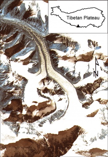
Fig. 1. Advanced Land Observing Satellite (ALOS) 2007 image of ERG. The location of ERG is shown as a triangle in the inset.
In May 1960, a shallow borehole was drilled at 5400 m a.s.l. on Rongbuk Glacier, ∼1 km west of ERG, and the ice temperature at 10 m depth was measured as −2.1°C (TSECAS, 1975). Ice temperature was also measured in a deep crevasse at 6325 m a.s.l. on ERG in April 1968, which suggested a value of −12.2°C at 25.5 m depth (TSECAS, 1975). Ice temperature measurements were also obtained at discrete depths in a 108.8 m borehole drilled to bedrock at 6518 m a.s.l. on ERG in September/October 2002. These borehole ice temperatures were −9.6°C at 20 m depth and −8.9°C at 108.8 m depth (Reference HouHou and others, 2007; Reference XuXu and others, 2009). Despite these few in situ measurements indicating ice temperatures well below the pressure-melting point, which is approximately −0.09°C at 100 m ice depth, Reference HuangHuang (1999) speculated that large valley glaciers in the Qomolangma region likely sustained temperate ice zones (TIZ) in the basal ice of their ablation zones.
Prior to 2005, ice velocity measurements on ERG had only been made on two cross sections at 5600 and 5900 m a.s.l. over a 4 month period in summer during the 1959–60 expedition. These observations suggested that ice velocity varied from several metres to tens of metres per year (TSECAS, 1975). Most existing in situ measurements of ERG surface velocity were obtained during 2005–11.
Due to logistic difficulties, it is hard to drill and instrument boreholes for the measurement of ice temperature and velocity profiles at as many locations as we would have wanted. Numerical modelling, validated against the sparse observational data, thus offers an alternate approach to derive complete distributions of englacial temperature and velocity. In order to develop a fully transient glacier dynamic model for projecting future changes of glacier meltwater runoff, a validated diagnostic ice flow model must first be developed. This is the primary aim of this paper.
In this paper, we use a two-dimensional (2-D) higher-order thermomechanical flowband model to study the diagnostic behaviour of ERG. We first describe the model input data (i.e. ice surface velocity, glacier geometry, surface air temperature and geothermal heat flux), and then briefly describe the numerical model that we employ. We adopt a phenomenological friction law to simulate the basal sliding in the ice flow model and use a numerical iteration scheme to determine the locations of cold–temperate transition surface (CTS) in the temperature model. Finally, we present and discuss the major findings of this research, which include the model sensitivity experiments, the simulated present-day ice temperature and velocity distribution along the main flowline (MFL) of ERG, and their comparison with available in situ observations.
2. Model Input
2.1. Ice surface velocity
Due to the difficulties of conducting fieldwork in heavily crevassed areas, in situ ice velocity data are sparse for ERG. We provide some in situ ice surface velocities for ERG, inferred from stake displacements measured between repeat stake surveys using the GPS. These in situ velocity observations include annual velocities observed between May 2007 and May 2008, summer velocities observed between April and October in 2009 and 2010, and the winter velocities observed between October 2010 and June 2011. The locations of the surveyed stakes (2007–11) along the MFL are shown in Figure 2. Over a large portion of the glacier (km 2.4–6.5 from the glacier head), only summer velocity data exist (Fig. 3). Based on the observation that the summer velocity at 5775 m a.s.l. (km 9.1) is approximately twice the winter velocity, we estimate mean annual velocities by multiplying summer velocities by a factor of 0.75 (Fig. 3).

Fig. 2. Map of ERG. The contours are produced from a 1 : 50 000 topographic map made in 1974. The black thick line and thin dotted lines denote the main flowline (MFL) and the boundaries of tributaries, respectively. Black dots denote stake sites for ice surface velocity measurements along the MFL. BH1 (6518 m a.s.l.), BH2 (6350 m a.s.l.) and BH3 (5710 m a.s.l.) denote ice boreholes (red squares). The blue lines, L1, L2, L3 and L4, are ground-penetrating radar survey lines.

Fig. 3. In situ ice surface velocity observations along the MFL of ERG. The mean annual velocities are estimated by mutiplying the summer season velocities by 0.75.
2.2. Glacier geometry
In May 2009, a ground-penetrating radar (GPR) survey was conducted on ERG using a pulseEKKO PRO radar system with a centre frequency of 100MHz (Reference Zhang, Xiao, Qin, Hou and DingZhang and others, 2012). Both the antenna separation and step size were set to 4 m. Since the terminus of ERG is covered by up to several metres of debris, a common-midpoint (CMP) survey was performed to calibrate radar velocity below 5600 m a.s.l. (km 11–12). The average radar velocity inferred for the thick debris-covered region was 0.13–0.15 m ns−1 (Reference Zhang, Xiao, Qin, Hou and DingZhang and others, 2012), and a radar velocity of 0.168 m ns−1 was assumed in the clean ice zone (e.g. Reference Bradford, Nichols, Mikesell and HarperBradford and others, 2009). The maximum ice thickness along the MFL of ERG is ∼320 m, and the average is ∼190 m.
The cross-sectional glacier shape may be described by a power law function, z(y) = pyq , where y and z are the horizontal across-flow and vertical distances from the lowest point of the cross section, and p and q are constants. q is commonly used as an index of the steepness of the valley side, while p is a measure of the width of the valley floor (Reference SvenssonSvensson, 1959; Reference GrafGraf, 1970). For ERG, we find that q varies within the range 0.7–1.3 and p has an exponential relation with q, –ln (p) = 7.1 × q − 6.5 (Reference Zhang, Xiao, Qin, Hou and DingZhang and others, 2012). This indicates that the cross-sectional profile of ERG may be regarded as ‘V’-type.
Few GPR survey lines overlapped with the MFL above 6300 m a.s.l. (km 0–2.4). The MFL bed profile above 6300 m a.s.l. was therefore inferred by transposing data from nearby GPR survey lines based on the cross-sectional shape of the glacial valley perpendicular to ice flow (Reference Zhang, Xiao, Qin, Hou and DingZhang and others, 2012). In the elevation band between 6000 and 6300 m a.s.l. (km 2.4–6.5), where the glacier surface is composed of large ice seracs, ice thickness was inferred by cubic interpolation of upstream and downstream observations. A central moraine ridge divides the glacier into two deeply incised adjacent channels between 5800 and 6000 m a.s.l. (km 6.5–8.8; Fig. 1; Reference Zhang, Xiao, Qin, Hou and DingZhang and others, 2012). When calculating the ice thickness and glacier width along the MFL we ignore all tributaries (Figs 2 and 4).

Fig. 4. (a) The glacier geometry along the MFL of ERG. The thin and thick lines denote glacier surface and base, respectively. (b) The glacier width along the MFL of ERG.
2.3. Surface air temperature
During the 2008 Olympic torch relay, several automatic weather stations, ranging in elevation from 5207 to 7028 m a.s.l., were installed by the Chinese Academy of Sciences at Qomolangma. A HOBO automatic weather station deployed at 5708 m a.s.l. (km 9.8) recorded a mean annual air temperature of −5°C during the 2009–11 period. We use the average environmental lapse rate at ERG recorded by these stations, −0.72°C per 100 m rise in elevation (Reference Yang, Zhang, Qin, Kang and QinYang and others, 2011), to calculate the mean annual air temperature at different elevations on ERG.
2.4. Geothermal heat flux
The ice temperatures in a borehole drilled to bedrock near the flow divide in 2002 (BH1; Fig. 2) were −9.6°C and −8.9°C at depths of 20 and 108.8 m, respectively (Reference HouHou and others, 2007; Reference XuXu and others, 2009). According to snow-pit measurements, the mean annual surface mass balance at BH1 in 2002 was ∼400 mm a−1 (Reference HouHou and others, 2007). The drilling site was selected where there was negligible horizontal ice velocity (Reference HouHou and others, 2007; Reference XuXu and others, 2009). Similar to the 2-D energy-balance equation described in Section 3.2 below, a one-dimensional (1-D) heat conduction model (Reference Cuffey and PatersonCuffey and Paterson, 2010) was used to infer the geothermal heat flux required to satisfy BH1 ice temperature observations with known ice geometry and surface mass balance. The 1-D heat conduction model suggests a geothermal heat flux of ∼18.5 mW m−2. This geothermal heat flux was applied to the entire ERG model domain.
3. Model Description
3.1. Ice flow model
Here we briefly describe the 2-D higher-order flowband model that we use in this study. A complete model description can be found in Reference Pimentel, Flowers and SchoofPimentel and others (2010) and Reference Flowers, Roux, Pimentel and SchoofFlowers and others (2011). In a Cartesian coordinate system (where x is the horizontal axis oriented down-glacier and z is the vertical axis oriented upward), the 2-D force balance equations are
where σij (for i, j = x, z) are the components of the stress tensor, ρ is ice density, g is gravitational acceleration and F is the lateral shear stress gradient that is missing in the standard 2-D (plane-strain) force balance equations. Constants used in the numerical model are listed in Table 1. Based on the hydrostatic approximation and a stress-free condition at the glacier surface (Reference BlatterBlatter, 1995), we express the force balance equation as
where ![]() (for i, j = x, z) denotes the components of the deviatoric stress tensor and s is the ice surface elevation. Following Reference Flowers, Roux, Pimentel and SchoofFlowers and others (2011), we assume no lateral slip or slide along valley walls, and parameterize F as
(for i, j = x, z) denotes the components of the deviatoric stress tensor and s is the ice surface elevation. Following Reference Flowers, Roux, Pimentel and SchoofFlowers and others (2011), we assume no lateral slip or slide along valley walls, and parameterize F as
where η is temperature and strain-rate-dependent effective viscosity of ice, u is the horizontal velocity along the x direction and W(x, z) is the flowband half-width. We take the y-axis orthogonal to the MFL with y = 0 at the MFL. The effective viscosity of ice is given by
where ![]() , is effective strain rate,
, is effective strain rate, ![]() is a small value used to avoid numerical singularity, n is the flow law exponent, and A is a temperature-dependent flow law parameter, described by the Arrhenius-type relation
is a small value used to avoid numerical singularity, n is the flow law exponent, and A is a temperature-dependent flow law parameter, described by the Arrhenius-type relation

with A 0 a reference flow law parameter, Q the creep activation energy of ice, R the universal gas constant and T the ice temperature (K). The effective strain rate can be calculated as (Reference Greve and BlatterGreve and Blatter, 2009)

where v is the horizontal velocity along the y direction. Taking ∂v/∂y = u/W · ∂W/∂x (Reference NyeNye, 1959; Reference Flowers, Roux, Pimentel and SchoofFlowers and others, 2011), we rewrite Eqn (3) as follows:

where the effective viscosity of ice can be expressed as

Table 1. List of parameters and values prescribed for the experiments, and some other symbols

3.2. Ice temperature model
In order to assess the present-day ice temperature distribution along the MFL of ERG, we assume a thermal steady-state condition, whereby the 2-D energy-balance equation including the horizontal diffusion becomes (Reference PattynPattyn, 2002)

where K is the conductivity of ice, c is the heat capacity of ice and E is the strain heat produced by internal deformation (Reference Greve and BlatterGreve and Blatter, 2009)
The vertical ice velocity, w, is solved directly from the incompressibility condition (e.g. Reference PattynPattyn, 2002)

where b is the elevation of the glacier bed.
The pressure-melting-point of glacier ice, T pmp, is described by the Clausius–Clapeyron relation
where T 0 is the triple point of water and β is the Clausius–Clapeyron constant. A CTS is located at the depth where ice colder than T pmp is in contact with temperate ice at T pmp. The ice flowing across the CTS can be assumed to have a negligible water content where cold ice flows into the temperate ice zone (TIZ) (Reference Blatter and HutterBlatter and Hutter, 1991; Reference Greve and BlatterGreve and Blatter, 2009). Thus, in this case, the ice temperature gradient at the CTS is equal to the Clausius–Clapeyron gradient (Reference Funk, Echelmeyer and IkenFunk and others, 1994). The temperate ice flowing across the CTS from the TIZ into cold ice, however, cannot be assumed to have a negligible water content. The trace water contained in the temperate ice will refreeze and release latent heat Q r as it crosses the CTS:
where θ is the fractional water content of the temperate ice, ρ w is the density of water and L is the latent heat of freezing of water (Reference Greve and BlatterGreve and Blatter, 2009). Thus, in this case, the ice temperature gradient at the CTS may be described by (Reference Funk, Echelmeyer and IkenFunk and others, 1994)
Due to the presence of Q r, the vertical location of the CTS must be determined by numerical iteration (Reference Funk, Echelmeyer and IkenFunk and others, 1994; see Section 3.4 below).
3.3. Boundary conditions
In the ice flow model, the upstream and downstream boundary conditions are both zero ice velocities. The upper boundary condition is a stress-free surface (Reference BlatterBlatter, 1995; Reference Flowers, Roux, Pimentel and SchoofFlowers and others, 2011) while the lower boundary condition is a phenomenological friction law (Reference Gagliardini, Cohen, Råback and ZwingerGagliardini and others, 2007; Reference Flowers, Roux, Pimentel and SchoofFlowers and others, 2011)

where τ b is the basal drag, Γ is a constant, u b is the sliding velocity, N is the basal effective pressure, λ max is the dominant wavelength of bed bumps and m max is their maximum slope. We take λ = 0:84 m max, assuming a sinusoidal bedrock geometry (e.g. Reference Gagliardini, Cohen, Råback and ZwingerGagliardini and others, 2007). The basal effective pressure N is defined as
where H is ice thickness and P w is the basal water pressure. We use a factor ϕ to represent the effective basal pressure as a fraction of total ice overburden pressure. The basal drag is defined as the sum of all resistance stress at the glacier bed (Reference Van der Veen and WhillansVan der Veen and Whillans, 1989; Reference PattynPattyn, 2002). Neglecting the basal melt rate, the vertical velocity at the glacier bed can be calculated according to the basal kinematic boundary condition (Reference Greve and BlatterGreve and Blatter, 2009)
The upper boundary condition of the ice temperature model is mean annual air temperature, while the lower boundary condition is a prescribed geothermal heat flux, G:
At the glacier head (km 0), the vertical ice temperature profile is derived from a 1-D solution of the energy-balance equation assuming negligible horizontal advection.
3.4. Numerical method
The numerical calculation of u may produce a singularity at the glacier bed (Eqn (8)), where W = 0, if we parameterize the shape of a glacier valley using a power law function, z(y) = pyq . To avoid a numerical singularity, we prescribe W at the glacier bed, W(x, b), as a small fraction, χ, of the nonzero W of the gridpoint above, W(x, b + Δz):
Neglecting the contribution of ![]() and
and ![]() to the basal drag (Reference Adhikari and MarshallAdhikari and Marshall, 2011), we can express the basal sliding boundary condition as follows (Reference Pimentel, Flowers and SchoofPimentel and others, 2010):
to the basal drag (Reference Adhikari and MarshallAdhikari and Marshall, 2011), we can express the basal sliding boundary condition as follows (Reference Pimentel, Flowers and SchoofPimentel and others, 2010):

where l is the iteration number.
For the temperature model, the CTS depth is determined differently where vertical ice velocities at the CTS are downward and upward. Under the condition in which cold ice flows downwards across the CTS into the TIZ, if the calculated ice temperature exceeds the pressure-melting point (i.e. T > T pmp), the ice temperature is set to the pressure-melting point. This assumes that any excess heat is absorbed by the latent heat associated with melting. Under the condition in which temperate ice flows upwards across the CTS into the cold ice zone, however, the latent heat released by refreezing, Q r, at the CTS must be taken into consideration. If Q r is sufficient to raise the ice temperature of the gridpoint above the CTS to the pressure-melting point,
the CTS is raised by one gridpoint. The vertical ice temperature profile is iteratively recalculated with the modified CTS grid position until the CTS node position no longer changes between iterations (Reference Funk, Echelmeyer and IkenFunk and others, 1994).
For numerical convenience, we adopt a terrain-following coordinate system (e.g. Reference PattynPattyn, 2003)
with ζ = 0 at the glacier bed and ζ = 1 at the glacier surface. We apply a 51 (horizontal) × 21 (vertical) grid to the longitudinal cross-section profile of ERG. A second-order, gridpoint-centred, finite-difference scheme is applied to discretize Eqn (8). The energy-balance equation (Eqn (10)) is discretized using first-order upstream differences in the horizontal, and node-centred differences in the vertical. The ice temperature field is sequentially solved, in column-bycolumn fashion, from the glacier head to the terminus. Ice viscosity and temperature are initialized as η = 1013 Pa s (Reference Zwinger and MooreZwinger and Moore, 2009) and −5°C (based on in situ ice temperatures at boreholes BH1, BH2 and BH3), respectively. Both the ice temperature and velocity fields of the entire longitudinal cross-section profile are then determined by a relaxed Picard subspace iteration scheme following Reference De Smedt, Pattyn and De GroenDe Smedt and others (2010). Denoting
![]() and u
l
as the lth velocity field from true Picard iteration and the relaxed Picard subspace iteration, respectively, we have good numerical convergence when the velocity field satisfies the condition (Reference De Smedt, Pattyn and De GroenDe Smedt and others, 2010)
and u
l
as the lth velocity field from true Picard iteration and the relaxed Picard subspace iteration, respectively, we have good numerical convergence when the velocity field satisfies the condition (Reference De Smedt, Pattyn and De GroenDe Smedt and others, 2010)

4. Results and Discussion
4.1. Model sensitivity
We perform diagnostic modelling experiments to simulate the present-day ice velocity and temperature distribution along the MFL of ERG. Our model has six free parameters: (1) friction law parameter m max, (2) friction law parameter λ max, (3) effective basal pressure fraction ϕ, (4) basal width fraction χ, (5) glacial valley shape index q and (6) fractional water content in temperate ice θ. In a series of numerical experiments (Figs 5 and 6), we explore the independent impact of each of these parameters on the model sensitivity by varying only one at a time while holding the other five fixed at the values we use in our model (m max = 0.2, λ max =5 m, ϕ = 1, χ = 1/2, q = 1, and θ = 1%).
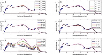
Fig. 5. Sensitivity experiments of ice velocity along the MFL. We vary only one parameter at a time, while holding the other five fixed at the values we use in our model (m max = 0.2, λ max = 5 m, ϕ = 1, χ = 1/2, q = 1 and θ = 1 %). The solid, dotted and black dashed lines denote surface velocity, basal sliding velocity and surface velocity under a no-slip scenario with q = 1 (V-shaped glacial valley), respectively. The solid circles denote in situ measurements of mean annual surface ice velocity obtained from the stakes located on or near the MFL (see Fig. 2).
Fig. 6. Sensitivity experiments of the size of TIZ (dashed lines). The parameter setting is the same as in Figure 5.
The friction law parameters, m max and λ max, represent the maximum slope and wavelength of basal roughness, respectively. Basal sliding velocity, u b, is expected to increase as m max decreases (Fig. 5a) and λ max increases (Fig. 5b) (Reference Flowers, Roux, Pimentel and SchoofFlowers and others, 2011). For a sinusoidal glacier bed with cavities, we may find that m max is raised to a greater power (n + 1, Γ nm max) than λ max (1) in the friction law (Reference SchoofSchoof, 2005; Reference Flowers, Björnsson, Geirsdóttir, Miller and ClarkeFlowers and others, 2007; Reference Gagliardini, Cohen, Råback and ZwingerGagliardini and others, 2007; Eqn (21)). As a result, u b is more sensitive to m max than λ max (Fig. 5a and b).
The effective pressure, N, determined as the ratio between ice and water pressures, appears to have little influence on basal sliding for such a narrow glacial valley (Fig. 5c). From Eqn (21) we know that the value of ∂u/∂z(b), which is coupled to the momentum balance equation (Eqn (8)), depends on the relative magnitudes of u b /Nn and λ max A/m max. Thus, a relatively narrow glacial valley (small u b), a relatively large ice thickness (large N) and flow law parameter may produce a u b /Nn term that is negligible in comparison to the magnitude of the λ max A/m max term. This would render the influence of the effective basal pressure factor, ϕ, less important. This is possibly the reason why Reference Flowers, Roux, Pimentel and SchoofFlowers and others (2011) found that values of m max and λ max strongly affected their selection of the best value of N for a good simulation of ice velocities.
We further see the critical role that glacial valley plays in modulating basal sliding in Figure 5d and e. As the glacier bed becomes flatter, which is parameterized by increasing the χ parameter, basal sliding velocity increases. Modelled ice surface velocity appears to be most sensitive to varying the cross-sectional valley profile via q. Varying q between 0.8 and 1.2 produces the widest velocity sensitivity range of the six parameters examined. Modelled ice temperature, which is coupled to modelled ice velocity, is also more sensitive to the prescribed cross-sectional valley profile (Fig. 6e) than m max, λ max and N (Fig. 6a–d). Figure 7 provides a comparison between modelled and observed ice temperatures in shallow boreholes, BH2 (17.5 m deep at 6350 m a.s.l., km 1.7) and BH3 (18 m deep at 5710 m a.s.l., km 9.8), over a range of chosen values of q.
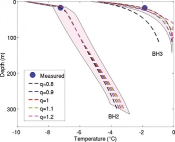
Fig. 7. Comparison of measured and modelled ice temperature at BH2 and BH3. The shaded areas denote ice temperature ranges for ±1 gridpoints upstream and downstream of BH2 and BH3 with q = 1.
We assume that the rate factor A is independent of water content θ (Eqn (6)), so the sensitivity of u b to water content, θ, is small (Fig. 5f). A significant increase in water content only slightly increases the length of the TIZ (Fig. 6f). We attribute this insensitivity to relatively small vertical ice velocities (<0.1 m a−1 in the TIZ), which render the latent heat term of the heat equation insensitive to most parameters, including water content (Eqn (14)).
Based on the sensitivity experiments described above, we adopt m max = 0.2, λ max = 5 m, ϕ = 1 (no basal water pressure), χ = 1/2, q = 1 (a V-shaped glacial valley) and θ = 1 % (typical of temperate ice; Reference Cuffey and PatersonCuffey and Paterson, 2010) as the parameter suite that best simulates the present-day ice velocity and temperature distributions of ERG.
4.2. Model results
Using the numerical model and parameter suite described above, we simulate the present-day ice velocity and temperature distributions in the longitudinal cross-sectional profile along the MFL of ERG (Fig. 8).
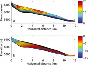
Fig. 8. Modelled distribution of (a) horizontal ice velocity (m a−1) and (b) temperature (°C) along the MFL of ERG. The thick blue line denotes the CTS.
The modelled ice surface velocities generally agree well with the observed mean annual velocities under the parameter suite we adopt (Fig. 5). However, since the numerical simulations ignore the influxes stemming from ERG tributaries, the modelled ice surface velocities do underestimate observed ice surface velocities at km 2, where the largest tributary converges with the MFL (Fig. 2). Figure 5 suggests that basal sliding may influence ice flow over a more extensive region than the TIZ, which was also suggested by Reference Pimentel, Flowers and SchoofPimentel and others (2010). The observation of seasonal velocity variations at 5775 m a.s.l. (km 9.1; see Section 2.1) provides independent support for the notion of a basal TIZ (Reference ColganColgan and others, 2012). Overall, however, basal sliding likely contributes a minor portion (<20%) of mean annual ice velocity at ERG. The flow of ERG is dominated by slow internal deformation. The internal deformation rate is slow mainly due to the relatively small ice thickness (<320 m), the relatively narrow glacier valley (large lateral drag) and high-elevation (cold atmosphere) setting of ERG. The narrow glacial valley cross section of ERG is itself independent support for relatively little basal sliding. Significant basal sliding would be expected to enhance basal erosion (Reference HarborHarbor, 1992, Reference Harbor1995), which would have allowed ERG to have evolved to the broad U-shaped valley cross section characteristic of alpine glaciers.
The model suggests the existence of an extensive TIZ, ∼6 km in length from around 5700 to 6200 m a.s.l. (km 4–10), in the basal ice of the ERG upper ablation zone. The accumulation zone and the terminus of ERG, however, are still underlain by cold ice. Thus, we suggest ERG is a polythermal glacier. Modelled ice temperature agrees well with the deepest available ice temperature measurements in two shallow ice boreholes (BH2 at 17.5 m and BH3 at 18 m) at 6350 (km 1.7) and 5710 m a.s.l. (km 9.8) (Fig. 7). No deep, near-bedrock, ice temperature measurements are presently available for comparison with modelled ice temperature. The GPR data obtained in May 2009, however, exhibit reflectance variations that we interpret as resulting from differences in the thermal character of cold up-glacier and warm down-glacier regions (Figs 2 and 9). In the up-glacier region, a continuous glacier bed is clearly visible in ‘clean’ radar data above 6300 m a.s.l. (km 0–2.4), which we interpret as evidence of cold basal ice (e.g. Reference Irvine-Fynn, Moorman, Williams and WalterIrvine-Fynn and others, 2006). In the down-glacier region, radar energy is scattered. The radargram near the glacier bed appears noisy near the terminus, in the 5760–6020 m a.s.l. elevation band (km 5.3–9.2). We interpret this region of scattered radar energy as independent support of a substantial basal TIZ (e.g. Reference Irvine-Fynn, Moorman, Williams and WalterIrvine-Fynn and others, 2006).

Fig. 9. GPR energy is scattered near the glacier bed in the downstream ablation zone (L1 and L2), which we interpret as indicating the presence of temperate basal ice. In the upstream portion of ERG (L3 and L4), a clean glacier bed can be identified, suggesting the presence of cold basal ice. The locations of L1–L4 are shown in Figure 2.
For ERG, the existence of a relatively large warm base is partly due to its small accumulation basin. From the in situ observations during 2009–11, the present-day surface mass-balance equilibrium-line altitude of ERG is ∼6400 m a.s.l. (km 1), and the accumulation zone presently comprises only 8% of the total glacier length. As a result, the advection of cold ice from the accumulation zone only influences (i.e. ‘cools down’) the ice temperature of a very small portion of the ablation region.
As a sensitivity test to examine the permanence of the TIZ, we decreased geothermal heat flux and mean annual air temperature to simulate a much colder environmental setting. This test demonstrated that a small TIZ (thinner than the thickness of one grid layer) exists in the downstream ablation zone (km 7–10), even under a prescribed mean annual air temperature at 5708 m a.s.l. (km 9.8) of −7°C (2°C lower than the present surface air temperature; Fig. 10a) or a prescribed geothermal heat flux of only 9 mW m−2 (around half of the present geothermal heat flux; Fig. 10c). Accordingly, the TIZ grows larger when we prescribe larger geothermal heat fluxes and surface air temperatures (Fig. 10b and d). On ERG, the size of the TIZ appears to be more sensitive to surface air temperature than to geothermal heat flux (Fig. 10). Thus, we speculate that basal temperate ice zones are likely a common feature of large valley glaciers like the ERG in the Qomolangma region.

Fig. 10. Sensitivity studies of the ERG TIZ size under scenarios of (a) G = 18.5 mW m−2, T 5708 = −7°C; (b) G = 18.5 mW m−2, T 5708 = −3°C; (c) G = 9 mW m−2, T 5708 = −5°C; and (d) G = 37 mW m−2, T 5708 = −5°C. The temperature values are in Celsius. The thick blue lines denote the CTS.
4.3. Model limitations
Although the true cross-sectional valley shape of ERG is believed to approximate a V-shape (Reference Zhang, Xiao, Qin, Hou and DingZhang and others, 2012), imposing an idealized V-shaped cross section in our model is an assumption that is only supported by inferences, not actual observations. Since basal water pressure and the true bed geometry are not known, ϕ, χ and the bed roughness parameters in the friction law, i.e. m max, λ max and Γ, cannot be constrained based on the observations. To address this limitation, we have examined a wide range of values for these parameters in our sensitivity experiments. Additionally, as our model ignores all tributaries, we cannot assess the lateral flow effects stemming from tributary convergence. Furthermore, because of the lack of 3-D glacier geometry information, we use a 2-D ice flow model. As a compromise, we parameterize lateral drag with the glacier width variations. Finally, the ice temperature model is 2-D, and thus neglects horizontal advection in the y direction. In our 2-D model, it is difficult to simulate the lateral sliding since we lack any knowledge of the distribution of CTS along the glacial valley walls. However, this may not introduce much error because (1) lateral sliding is an unimportant factor influencing ice flow compared to glacier width (Reference Pimentel, Flowers and SchoofPimentel and others, 2010) (except for the cases of glaciers with detached side walls; Reference Adhikari and MarshallAdhikari and Marshall, 2012) and (2) ERG is a relatively cold glacier with narrow cross-sectional valleys and thus small sliding velocities.
5. Conclusions
For large alpine valley glaciers with few in situ observations available, it is difficult to construct a suitable glacier model with both reliability and simplicity. The 2-D higher-order thermomechanical flowband model presented here requires much fewer input data than a 3-D high-order or full-Stokes model. Nevertheless, it can simulate most glacier dynamic features (e.g. the longitudinal stress gradient coupling, lateral drag, basal sliding velocity and CTS), and thus is a good option for large glacier modelling.
The strong ablation, due to large solar radiation and a warming climate (TSECAS, 1975; Reference HockHock, 2003; Reference Pellicciotti, Brock, Strasser, Burlando, Funk and CorripioPellicciotti and others, 2005; Reference Huss, Funk and OhmuraHuss and others, 2009), leads to a small accumulation zone on ERG. As a result, the vertical velocity is presently upwards throughout most of the glacier, facilitating the upward advection of warm basal ice throughout the oversized ablation zone. There are at least two important implications of a basal TIZ. Firstly, temperate ice allows an active englacial hydrology system to exist (Reference Fountain and WalderFountain and Walder, 1998). An active englacial hydrology system allows surface ablation to route through a glacier without being retained by refreezing. This has implications for land-terminating Himalayan glaciers whose mass loss occurs only by surface ablation and runoff. Secondly, temperate ice and meltwater facilitate basal sliding (Reference Bartholomaus, Anderson and AndersonBartholomaus and others, 2008). A potential enhancement of basal sliding with warming climate is expected to transport more ice to lower-elevation areas where higher surface ablation occurs.
While it has been speculated that the ablation zones of large continental valley glaciers in the Qomolangma region contain basal ice at the pressure-melting-point (TSECAS, 1975; Reference HuangHuang, 1999), our study is the first modelling support for this hypothesis. In addition, this study is also the first to model a large valley glacier located on the northern slope of the Himalayan range. Work is currently underway to develop a fully transient prognostic version of the model, in order to predict the ice geometry, velocity and temperature of ERG under future climate scenarios.
Acknowledgements
This study is funded by National Fundamental Research Project (973) of China (2007CB411503) and National Science Foundation of China (NSFC). We are grateful to all members of the scientific expedition to Qomolangma for their dedication to the extraordinarily hard fieldwork. We also thank Konrad Steffen for supporting T.Z.’s visit to CIRES to learn glacier modelling. We thank Heinz Blatter, Mathieu Morlighem, Arne Keller, Surendra Adhikari, Ian Allison and an anonymous reviewer for their reviews of an earlier version of this paper. Weili Wang was our scientific editor.


