


Introduction
Melting, refreezing and the passage of liquid water into a snowpack can drastically change its physical and mechanical characteristics. The heterogeneities within a snowpack (ice-lensing, fingering, ponding and ice-crust formations) are often caused by the presence of liquid water and its percolation through the sub-freezing snow cover. Since liquid-water saturation combines liquid-water content and porosity, it is often used as an independent variable while modelling the meltwater percolation in snow (Reference ColbeckColbeck, 1972, Reference Colbeck1973, Reference Colbeck1974, Reference Colbeck1975; Reference Denoth, Seidenbusch, Blumthaler, Kirchlechner, Ambach and ColbeckDenoth and others, 1979; Reference Ambach, Blumthaler and KirchlechnerAmbach and others, 1981; Reference BengtssonBengtsson 1982; Reference Colbeck and AndersonColbeck and Anderson, 1982; Reference McGurk, Kattelmann and KaneMcGurk and Kattelmann 1986; Reference Bøggild, Hellström and FrankensteinBøggild, 2006). We present a method to directly measure the water saturation in snow. This method is fast in operation and we can speedily record the saturation profiles from snow over a large area.
Hot calorimetric (Reference AkitayaAkitaya, 1978, Reference Akitaya1985) and freezing calorimetric (Reference Jones, Rango and HowellJones and others, 1983) methods have long been used to measure the liquid-water contents in the snow samples. Reference Kawashima, Endo and TakeuchiKawashima and others (1998) made a portable calorimeter to measure this quantity, and Reference DenothDenoth (1994) designed a moisture meter, based on change in the dielectric constant of snow due to variations in the the liquid-water content. Time-domain reflectometry (TDR), based on the interaction of a microwave pulse with liquid water, is yet another method used to measure liquid-water content (Reference Stein and KaneStein and Kane, 1983; Reference Camp and LabrecqueCamp and Labrecque, 1992; Reference Schneebeli, Flühler, Gimmi, Wydler, Läser and BaerSchneebeli and others, 1995; Reference Spaans and BakerSpaans and Baker, 1995; Reference LundbergLundberg, 1996; Reference Stein, Laberge and LévesqueStein and others, 1997; Reference Schneebeli, Coléou, Touvier and LesaffreSchneebeli and others, 1998). A flat-cable TDR system was used by Reference Stähli, Stacheder, Gustafsson, Schlaeger, Schneebeli and BrandelikStähli and others (2004) to estimate the liquid-water content and water equivalent of snow from a spatially distributed snow cover at a fixed installation. Finnish scientists made a ‘snow fork’ which can also be used to record the density and the water-content profiles of a snowpack in a region approximately 20 mm in diameter around the probe (Reference Sihvola and TiuriSihvola and Tiuri, 1986). The liquid-water content measured by these devices is at some fixed points rather than over a continuous depth (Reference Pfeffer and HumphreyPfeffer and Humphrey, 1998).
For the purpose of recording the vertical distribution of water saturation over a large area, existing methods of measuring the water contents are unfeasibly time-consuming. Additionally, a large number of sensors are required to obtain a saturation profile by digging a pit (which can also disturb the snow cover). We have developed a parallel-probe saturation profiler (PPSP) for accurate and fast recording of vertical saturation profiles within a snowpack. The basic physical principle behind the detection of liquid-water content utilizes the instantaneous absorption of electrostatic energy by water molecules (as electric dipoles), which is a consequence of their rotation from their initial random directions to the direction of an applied electric field. For simultaneous measurements of depth positions, an incremental encoder has been fabricated which is placed within the main housing of the instrument. A data logger can also be connected to the PPSP to store the data recorded under field and laboratory conditions.
Mechanism for Rotation of Water Dipoles Under External Electric Field
A water molecule (H2O) is polar in nature, due to the asymmetry in its charge distribution. When water molecules, or more specifically ‘water dipoles’, are intercepted by an external electric field, they tend to align in the direction of the applied field, as distinct from their initial random alignments. Figure 1a shows the random orientations of water dipoles in the absence of an external electric field. Figure 1b shows the orientations of water dipoles in the direction of the external electric field. The positive-charge ends of the dipoles orient towards the negative terminal of the applied electric field, and the negative-charge ends of the dipoles tend towards the positive terminal. As these electric dipoles are rotated by means of an external d.c. electric field, they absorb a certain amount of the energy from the applied field. As soon as all the dipoles are aligned in the direction of the field, no further energy is required to rotate them; the larger the number of dipoles intercepted by the applied electrical field, the more will be the energy absorbed. If the electric field is switched off, some of the water dipoles may become misaligned (Fig. 1c), but as soon as the field is switched on again, they will realign in the direction of the applied field. Since most of the dipoles are not strongly misaligned from their initial directions in the latter case, the amount of energy required to rotate the water dipoles is less than if the alignments were random. As on–off cycles are repeated, the amount of energy absorbed will slowly decrease and may finally approach a constant value after a few cycles.
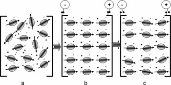
Fig. 1. Rotation of water molecules (as electric dipoles) under the action of an electric field.
Figure 2 shows the time-series power spectrum of water dipoles located in the pore space of a snow sample, prepared by partially saturating it with pure liquid water. The pore space of snow can be treated as dielectric cavities where water dipoles are trapped inside the pores. The change in potential energy of water dipoles due to rotation under the action of an electric field inside a complex dielectric cavity (e.g. a snow specimen) is treated mathematically in the Appendix. In our case, the applied d.c. electric field is of the order of 430 V m−1. When the electric field is switched on, the signal strength instantaneously shoots to a sharp peak value and then decreases to a minimum value. Thereafter it gradually increases again, and finally converts to a flat or linearly increasing curve. The initial instantaneous peak signal manifested in this power spectrum is a result of the energy absorbed while rotating the water dipoles due to the external electric field. As soon as all the water dipoles are aligned, no energy is required to rotate them and the signal strength immediately decreases (Fig. 2), tending to a minimum value. The total height of the signal is the sum of the energy required to rotate the dipoles and the energy required for ionic conduction caused by impurities inherently present in liquid water. Thus, the minimum value in the curve can be associated with the contaminant level of the water. Since the water molecules of the specimen are in contact with the sensor tips that act as anode and cathode, electrolysis will occur in the liquid water. This process dissociates the water molecule into a proton (H+)/hydronium (H3O+) ion and a hydroxyl (OH−) ion, leading to increased ionic conductivity in the specimen. The electrolysis process is slightly delayed relative to the dipole rotation process and the ionic contaminant conduction. The rate of generation of H+/H3O+ and OH− ions increases with time, giving rise to the increased ionic conduction represented by increased signal strength in the time-series power spectrum. As soon as equilibrium is established between the ions generated and the energy absorbed by them from the field, the linearly increasing curve and flat saturated curve are shown in the power spectrum (Fig. 2). In this case, our interest is centred on the initial instantaneous peak appearing in the power spectrum, arising due to the rotations of the water dipoles.
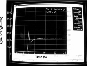
Fig. 2. Time-series power spectrum of water dipoles inside snow pore spaces.
Periodic Excitation of Water Molecules in Distilled Water
In order to verify the appearance of the initial instantaneous peak in the power spectrum, experiments were conducted using samples of high-grade distilled water by periodically exciting and de-exciting the specimen under the action of an external electric field at time intervals of 1, 2 and 4 s (Fig. 3a, b and c respectively). It is evident from Figure 3a that the height of the first peak signal (HFPS) due to first excitation is higher than the peaks arising due to subsequent excitations. This indicates that the maximum number of dipoles is rotated during the first cycle. The number of dipoles rotated decreases with the number of cycles. Similar observations are made from Figure 3b and c. In Figure 4a the variation of signal heights with excitation cycles is shown for excitation/de-excitation time periods of 12 s. The height of the signal, S h decreases with excitation cycles. A least-square fit exhibits a polynomial relation of order 3 in Figure 4b (S h = −0.6333 n 3 + 9.7 n 2 − 45.467 n + 70.8, where n is number of cycles and R 2 = 1). These observations show that during the first 2 s of excitation, the HFPS is related to the rotation of water dipoles from their initial random directions to the direction of the applied field; thereafter, the signal height is supported by the electrolysis process. Hence, the correct time interval to retrieve the HFPS is chosen to be, at most, 2 s.
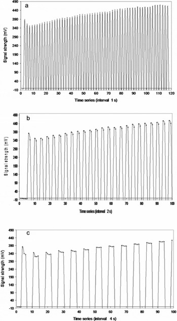
Fig. 3. Periodic excitation of water dipoles in a specimen of high-grade pure distilled water,under the action of an electric field of periods (a) 1 s, (b) 2 s and (c) 4 s.
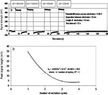
Fig. 4. Variation of peak signal height under consecutive cycles of electric field. (a) Power spectrum under consecutive cycles. (b) Peak signal height vs number of cycles.
Development of Parallel-Probe Saturation Profiler
Figure 5 is a schematic diagram of the PPSP that comprises two vertically moving parallel probes of stainless-steel tubes (length 90 cm, diameter 9 mm). These probes are fixed parallel to each other so that they can move simultaneously in the vertical direction. One sensor detects the liquid-water content while the other records the depth position inside the snowpack. The lower ends of the probes are attached to two copper tips (Fig. 5, label 1) which are used as electrical sensors. These sensors are of conical shape (cone angle 56°, cone height, 7 mm). The sensor tips (tip-to-tip distance 15 mm) act as electrodes, establishing a point-to-point communication between them. For better electrical conduction, both sensors are connected by Teflon-coated cables of extremely low electrical resistivity (Fig. 5, label 2) connecting to the data acquisition system. When a porous material, partially or fully saturated by liquid water, is located between the sensor tips and is intercepted by the electric field emanating from these terminals, the HFPS can be recorded.
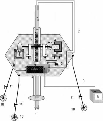
Fig. 5. Schematic diagram of PPSP. Labels are: 1. sensor tips; 2. data acquisition cable; 3. micro-controller and data acquisition system; 4. moveable handle; 5. optical interrupter for position encoder (incremental); 6. encoder cable; 7. rack-and-pinion arrangement; 8. 12 V battery; 9. power cable (12 V d.c. supply); 10. supporting legs; 11. nuts and bolts to support legs; 12. toggle switch.
For simultaneous measurements of the depths corresponding to the measured saturation value, an incremental position encoder was also constructed. This uses a slotted optical interrupter to generate square-wave pulses at a 950 nm wavelength. In the optical interrupter (H21A1), a GaAs photo diode is used as an infrared emitter (IRE) and a silicon photo transistor is used as a photo detector. To prevent the stray effects of ambient light, daylight cut-off filters are also mounted over the photo diode. The slot width between the IRE and detector is 5 mm. A moveable handle attached to rack-and-pinion arrangement is used to move the probes in the vertical directions (Fig. 5, label 4). The other end of the handle is attached to a slotted chopper wheel (label 5) which passes through a ‘U’ slot in the optical interrupter. Electrical pulses are thus generated when the infrared (IR) beam falls on the IR sensor, passing through the slots of the wheel via a connecting cable (label 6). Generation of the square-wave pulses is possible only when the IRE, the slot of the wheel and the photo detector are all aligned in the same direction. There are eight optical slots in the wheel, so eight pulses are generated corresponding to each revolution. In one complete revolution the rack-and-pinion arrangement (label 7) can move vertically up to 56 mm, so the minimum distance travelled corresponding to one revolution is 7 mm. In the present case, the height of the sensor tips is also 7 mm. This distance can be further reduced by decreasing the pitch of the rack-and-pinion arrangement as well as the size of the electrical sensors and by increasing the number of slots in the wheel accordingly.
The PPSP has three supporting legs to hold the instrument over a slope or a levelled ground. To create better contact between the ground and the instrument legs, a perforated circular base is attached to each leg (Fig. 5, label 10). This reduces sinkage into a soft snow cover. The lower segments of the legs are detachable.
The main power supply to the data logger (Fig. 5, label 3) is a 12 V battery (Fig. 5, label 8), connected to the data logger via a lead (label 9). However, to supply both kinds of sensor (liquid-water and depth) the 12 V d.c. supply is converted into two separate 5 V d.c. power supplies, which can be regulated using IC 7805. The data logger can be connected via the cables (Fig. 5, labels 2 and 6) to the sensors (labels 1 and 5) for recording the transient potential drops across the electrical sensors corresponding to the number of square-wave pulses generated by the optical interrupter. The CR10X data logger (Campbell Scientific Ltd, UK) was selected, and programmed to record any voltage fluctuations across the sensor tips between 0 and 2500 mV in <1 s (up to 1/64 s). For data acquisition, data storage and online monitoring of the output data, the required application programs were developed using the EdLog programming environment (Campbell Scientific Ltd, UK). The execution interval for the programs was kept equal to 1/64 s. Calibration curves for liquid-water saturation (% vol.) as well as liquid-water content (% vol.) are calculated by these programs. The data logger can be interfaced to a computer via SC32A, an optically isolated RS232 interface, and to the PPSP via a RS232 interface. The block diagram of the electronic circuit used in the data acquisition system and in the encoder circuits is shown in Figure 6. Various components/accessories used in the fabrication of the above circuits are indicated against their label numbers (Fig. 6). The output data (labelled 26–27) comprise the penetration depth (cm), liquid-water saturation (% vol.) and liquid-water content (% vol.).
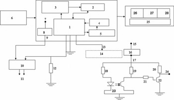
Fig. 6. Electronic block diagram of PPSP. Labels are: 1. micro-controller with data logger; 2. synchronization; 3. pulse counter; 4. calibrator; 5. measurements of signal strength; 6. 12 V d.c. power supply; 7. 12 V d.c. terminal; 8. IC 7805; 9. 5 V d.c.; 10. moisture/saturation sensors; 11. snow/soil; 12. R L = 22 KΩ; 13. pulse output; 14. encoder circuit; 15. 12 V d.c.; 16. IC 7805; 17. Vcc = 5 V; 18. 120 Ω; 19. 10 KΩ; 20. 10 KΩ; 21. 15 KΩ; 22. BC549; 23. H21A1; 24. output voltage V o; 25. output display; 26. depth position (cm); 27. liquid-water saturation (%); 28. liquid-water content (%).
Sample Preparation and Calibration Method
Detailed calibration work was carried out with the PPSP device, first inside a cold chamber (Fig. 7a) and then at different field stations of the Indian Snow and Avalanche Study Establishment (SASE; Fig. 7b), where various forms of snow (from extremely wet to dry) can be found. Samples were collected from a natural snowpack at Patsio, middle Himalaya, and immediately transported into an environmental cold chamber, the temperature of which was constantly maintained at 0 ± 1°C.For identification of various snow grain types, we refer to Reference ColbeckColbeck and others (1990). The temperature of the samples was tightly controlled near the freezing point by enclosing them in an ice bath.
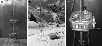
Fig. 7. Fabricated outlook of PPSP: (a) inside the cold chamber; (b) over an experimental test site at Patsio; and (c) the housing arrangement for data acquisition system and incremental encoder.
Laboratory Testing
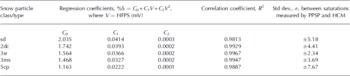
Small amounts of liquid water, maintained close to freezing point, were gently added to small dry snow samples and allowed to uniformly mix into the sample. The final mass and volume (if any volume change due to the addition of liquid water took place) were measured. Thus, the liquid-water content (% mass) of the snow sample can be calculated as the ratio of mass of liquid water to total mass of the snow sample, and this can be converted to liquid-water content (% vol.). The liquid-water saturation can be obtained from liquid-water content (% vol.) by dividing by the porosity of the specimen. Snow samples of known saturation and liquid-water content were prepared. The liquid-water contents of the samples were also measured by the hot calorimetric method (HCM) according to Reference AkitayaAkitaya (1985). The samples of known liquid-water content and water saturation were then measured using the PPSP inside the cold chamber at Patsio, to retrieve the time-series power spectrum. Figure 8a shows the recorded power spectrum of small rounded particles (class 3sr) corresponding to different percentages of saturation. The HFPS clearly has an increasing trend with percentage saturation of the snow sample, and it also increases with respect to the subsequent minima, with an increase in percentage saturation. The variation of HFSP (mV) is plotted as a function of liquid-water saturation (% vol.) as well as liquid-water content (% vol.) to obtain calibration curves. Figure 8b shows the calibration curves for 3sr snow samples, to correlate the saturation and the liquid-water content to the HFSP retrieved by PPSP. From these observations a very good correlation (R 2 ≈ 0.99) between the HFSP and the liquid-water saturation (% vol.) as well as the liquid-water content (% vol.) was found for small rounded snow particles. Similar correlations are observed for other kinds of snow particles (classes sd, 2dc, 3mx and 5cp; Reference ColbeckColbeck and others, 1990) (Table 1).

Fig. 8. (a) Variation of signal strength for small round snow particles (3sr type) retrieved by PPSP, as a function of liquid-water saturation (% vol). (b) Calibration curves corresponding to liquid-water content (lwc) (%) and to liquid-water saturation (%).
Table 1. Comparison between the coefficients of regression evaluated from a least-square fit of HFPS values on liquid-water saturation (% by volume), corresponding to different classes of snow particles
Preliminary Results and Discussions
Liquid-water saturations corresponding to the snow samples of different liquid-water contents were measured using PPSP and HCM. Results are shown in Figure 9. The comparison between saturation values measured by these two methods for 3sr snow shows that they agree with difference standard deviation, ±2.34%. Difference standard deviations for other snow samples are shown in Table 1. These experiments were repeated three times under the same conditions, after quenching the surface oxide formation over the sensor tips. The measured saturation values were also compared to known values of saturation. The samples with known saturation values were prepared by uniformly and gently adding the known amount of water (T = 0°C) into dry snow (T = 0°C). The results obtained are close to each other, with standard deviation ±3.46%. The repeatability of the measured values was also checked for various snow samples of known or unknown saturation values; the results show standard deviations between ±0.87% and ±5.53% for snow samples of different water saturations.
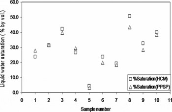
Fig. 9. Comparison between the saturation values of snow (3sr type) measured by HCM (Reference AkitayaAkitaya, 1985) and by PPSP.
Once laboratory testing of the PPSP was complete, the saturation profile of a homogeneous block of snow was measured. The block of snow was formed by uniformly depositing small rounded segregated grains of snow (grain size <1.0 mm) in a container at −22.0°C. After ageing for 48 hours, the block of snow was exposed to radiation generated by a sun simulator (radiation source comprised of two metal halide 2500 W lamps, with maximum intensity of radiation 1297 (±5%) W m −2, in an exposed area of 1.0 × 0.5 m2). Figure 10a shows the vertical profiles of liquid-water saturation and liquid-water content recorded from the block of snow, maintained at −4.0 ± 1°C (after 2 hours exposure to radiation of intensity 1300 W m −2). The saturation level increases at the bottom of the snowpack. Figure 10b shows the saturation profile of a natural snowpack with melting under natural solar radiation at Patsio during March 2008. Figure 10c presents the saturation profile of a snowpack under extreme melting conditions at Dhundi, Himachal Preadesh, India, during February 2007.
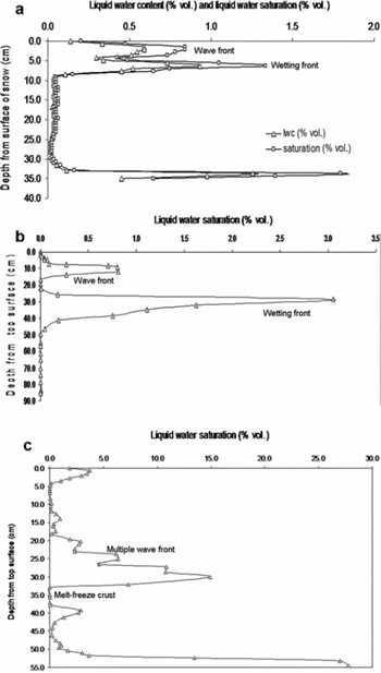
Fig. 10. Depth profiles retrieved by PPSP. (a) Liquid-water content (%) and liquid-water saturation (%) from a homogeneous block of snow exposed to the sun simulator. (b) Liquid-water saturation (%) of meltwater from a snow cover at Patsio, exposed under natural solar radiation. (c) Saturation profile of snowpack at extreme melting due to solar radiation, at Dhundi.
The accumulation of meltwater through several micro-channels to lower sub-layers of snow increases the saturation level accordingly. The percolation of meltwater in an unsaturated homogeneous snowpack comprises two kinds of percolation front, which Reference ColbeckColbeck (1975) categorized as the ‘wetting front’ (Fig. 10a) and the ‘wave front’ (Fig. 10b). In a heterogeneous snowpack, even under extreme melting conditions, the meltwater pattern cannot be clearly defined; however, multiple wave fronts can be seen in Figure 10c. Since meltwater accumulation finally takes place over the impermeable base or the ground; in some cases the saturation levels of the snowpack at the bottom layer are observed to be higher than at other depths. The formation of impermeable ice or melt–freeze crusts between different snow layers can also change the flow pattern. It is also clear from Figure 10c that there is an abrupt decrease in the liquid-water saturation values below 30 cm, indicating the presence of an impermeable crust of nearly 2.8 cm at this level. The snow-pit survey of this snowpack also confirmed the presence of a melt–freeze crust at 30–33.5 cm depth, with thickness nearly 3.5 cm.
The percolation depth, δ p, is the depth of the wetting front with respect to the top snow surface. In terms of saturation values, percolation depth is the vertical position, z, measured from the top surface of the snowpack, of a wetting front for which the saturation is 0 for all z≥ δ p. The wetting front can also be defined as a plane, f(x, y) with z = δ p, where x, y and z are the Cartesian coordinates. The wave-front and wetting-front velocities can also be estimated using the saturation profiles. We use the PPSP to investigate the spatial distributions of percolation depth in a melting snow cover that has previously undergone various melt–freeze cycles. Figure 11a shows an overview of the study site at Patsio, where the path ABC is the route along which saturation profiles were recorded. Patches of melting over the snow surface are visible, with some portions having undergone high melting rates while other portions are still dry. The PPSP measured percolation depth, relative to the snowpack depth, at each point along the path ABC is shown in Figure 11b. The depth of meltwater percolation depends on the topography and other aspects of the snow cover. Over the first 12 m, the average percolation depth was ∼10.5 cm. Between 14 and 34 m from A, it decreased to ∼4 cm, then it increased again (between 36 m and C) to ∼15 cm. The measurements show that most percolation occurred at our field stations on south- or southwest-facing slopes, and least on north- or northwest-facing slopes. A stratigraphic study of this snow-pack was conducted the next morning (after one refreeze cycle) adjacent to the curve ABC, and the positions of the wetting fronts were manually traced. There is good agreement between the results obtained using the PPSP and from the direct snow-pit survey.
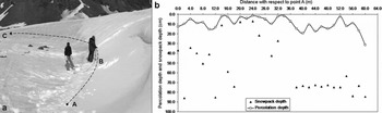
Fig. 11. Profiling the percolation depths of meltwater in a snowpack. (a) Overview of partially melted snow cover at Patsio. (b) Percolation depth relative to the snowpack height measured by PPSP.
Conclusions
The PPSP device can speedily record the penetration depth, liquid-water saturation and liquid-water content of a snow-pack. It is useful for both laboratory and field studies of snow and soil. The physical principle behind the instrument is the measurement of HFPS, possible due to the energy absorption during the rotation of a water molecule under the action of an external (d.c.) electric field. Other applications are possible (e.g. estimation of contaminants in water). Using the instrument for liquid-water saturation measurements is relatively fast, and the depth profile of a snowpack can be measured with an accuracy of ±5.53% and vertical depth resolution of 7 mm. It has been programmed to scan a 7 mm thick snow mass in 2 s, i.e. we can record one profile of saturation and liquid-water content from a 90 cm thick snow mass (nearly 128 measurements) in <5 min. For field studies a data logger powered by a 12 V battery can be used for real-time monitoring of liquid-water saturations/liquid-water contents. Thus, this instrument will be of interest to scientists involved in snow physics, hydrology, glaciology, soil science, agriculture and forestry.
Acknowledgements
We thank R.N. Sarvade, Director SASE, for his keen interest in the project, ‘HIMRAS’, and for financial and administrative support.We thank J. Singh for dedicated efforts during the development of the PPSP instrument. We acknowledge P.S. Negi and P.K. Srivastava for their critical suggestions. We thank R.K. Garg, R. Dass, S.K. Dewali and A. Aacharya for help and support during fabrication of the instrument, and V. Kumar and P. Kumar for support during sample collection and during the experimental work at Patsio. Finally, this paper would not have seen the light of day without the efforts of the scientific editor, P. Bartelt. We greatly appreciate his efforts.
Appendix Change in Potential Energy of Water Molecules Inside Pore Space of Snow Due to Rotation Under The Action of an Electric Field
A water-saturated specimen of snow can be treated as an anisotropic dielectric material filled with water molecules as electric dipoles. The pores are treated as dielectric cavities. Under the action of an external electric field, the change in potential energy, U m, of an electric dipole as it changes its orientation from an initial random direction, θ, to the direction of the applied field, θ = 0°, as shown in Figure 1, can be written as (Jackson, 1990)
where E m is electric field intensity inside the dielectric cavity and p 0 is the dipole moment of the water molecule at T = 0°C (p 0 = 6.17 × 10⁻³⁰ C m = 1.85 debye; Reference Moro, Rabinovitch, Xia and KresninMoro and others, 2006). If n is the total number of dipoles intercepted by the external field, E i, changing their orientations from initial directions (θ 1, θ 2, θ 3, … θn ) to the field direction, the change in potential energy will be

For n molecules, Equation (A2) can be approximated as
Reference Reitz, Milford, Christy, Reitz, Milford and ChristyReitz and others (1990) and Jackson (1990) showed that the electric field inside a dielectric cavity can be written as
where E is the intensity of an external electric field, P is the polarization and ε 0 is the permittivity of free space. P can be expressed in terms of dielectric constant, K, by
If N is the number of dipoles (water molecules) per unit volume and P m is dipole movement due to polarization,
then
and
where α is polarizability of the water molecule. From Equations (A4) and (A6),
Now using Equation (A4), we find

The dielectric polarizability, α, of water molecules can be deduced from the Clausius–Mossotti Langevin–Debye theory (Reference Reitz, Milford, Christy, Reitz, Milford and ChristyReitz and others, 1990):

where K B is Boltzmann’s constant and T is absolute temperature. Thus, we find the change in electrostatic potential energy, ΔU, of water dipoles in a dielectric medium like snow, while rotating them from their initial random direction, θ, to the direction of the electric field:

From Equation (A11) the change in potential energy of the water dipoles is proportional to the number of dipoles intercepted by the external electric field. The higher the number of dipoles rotated by the electric field, the higher the amount of electrical energy absorbed by them. The amount of absorbed energy can be shown to be proportional to the potential drop which is analogous to the signal strength shown in the signal response curve of the PPSP.


