


Introduction
The evolution of biological diversity is determined by the interplay between origination and extinction processes. Estimating the pace at which lineages appear and disappear is therefore a central question in macroevolution and paleobiology research. Inferring the processes underlying biodiversity patterns helps us understand what drives the wax and wane of taxa (Ezard et al. Reference Ezard, Aze, Pearson and Purvis2011; Quental and Marshall Reference Quental and Marshall2013), the effects of competition and other biotic interactions on diversity changes (Liow et al. Reference Liow, Reitan and Harnik2015; Pires et al. Reference Pires, Silvestro and Quental2017), and the dynamics and selectivity of mass extinctions (Peters Reference Peters2008). The process of taxonomic diversification is often modeled using birth–death stochastic models, in which the appearance of new lineages (e.g., species or genera) and their demise are characterized by origination and extinction rates (Kendall Reference Kendall1948; Keiding Reference Keiding1975; Nee Reference Nee2006). These parameters quantify the expected number of origination or extinction events per lineage per time unit (typically 1 Myr) (Foote Reference Foote2000; Marshall Reference Marshall2017).
In recent years, there have been considerable methodological developments in the estimation of diversification dynamics from phylogenies of extant taxa, in which the distribution of branching times calibrated to absolute ages are used to infer the parameters of a “reconstructed birth–death process” (e.g., Nee et al. Reference Nee, May and Harvey1994; Gernhard Reference Gernhard2008; Stadler Reference Stadler2009, Reference Stadler2013; Heath et al. Reference Heath, Hulsenbeck and Stadler2014). These methods are appealing, because large phylogenies of extant taxa are becoming increasingly available (e.g., Jetz et al. Reference Jetz, Thomas, Joy, Hartmann and Mooers2012; Zanne et al. Reference Zanne, Tank, Cornwell, Eastman, Smith, FitzJohn, McGlinn, O'Meara, Moles, Reich, Royer, Soltis, Stevens, Westoby, Wright, Aarssen, Bertin, Calaminus, Govaerts, Hemmings, Leishman, Oleksyn, Soltis, Swenson, Warman and Beaulieu2014; Rolland et al. Reference Rolland, Silvestro, Schluter, Guisan, Broennimann and Salamin2018; Chang et al. Reference Chang, Rabosky, Smith and Alfaro2019) and extend to taxa with limited fossil records, including hyperdiverse plant clades (e.g., Perez-Escobar et al. Reference Perez-Escobar, Chomicki, Condamine, Karremans, Bogarin, Matzke, Silvestro and Antonelli2017). Despite this methodological progress, estimating diversification dynamics from extant data remains challenging, particularly in terms of estimating realistic extinction rates (Liow et al. Reference Liow, Quental and Marshall2010a; Quental and Marshall Reference Quental and Marshall2010; Marshall Reference Marshall2017; Burin et al. Reference Burin, Alencar, Chang, Alfaro and Quental2019), although recent advances in integrating phylogenetic and paleontological data have clarified part of these apparent limitations (Silvestro et al. Reference Silvestro, Warnock, Gavryushkina and Stadler2018). Major limiting factors of phylogenetic approaches to infer origination and extinction rates are their dependence on accurate phylogenetic tree estimation (Warnock et al. Reference Warnock, Parham, Joyce, Lyson and Donoghue2015) and the fact that extant species represent, for most clades, a small fraction of the total diversity that has existed since their origination (Raup and Sepkoski Reference Raup and Sepkoski1984; Raup Reference Raup1986).
The fossil record provides the only direct evidence of past biodiversity and extinction and has therefore long been used to investigate diversification processes (Kurtén Reference Kurtén1954; Van Valen and Sloan Reference Van Valen and Sloan1966; Alroy Reference Alroy1996, Reference Alroy2008; Sepkoski Reference Sepkoski1998; Connolly and Miller Reference Connolly and Miller2001; Foote Reference Foote2001; Liow and Nichols Reference Liow, Nichols, Hunt and Alroy2010; Ezard et al. Reference Ezard, Aze, Pearson and Purvis2011). However, because the paleontological record is inevitably incomplete, fossil occurrences represent a biased representation of the past diversity, in which the sampled longevities of taxa are likely to underestimate their true life spans, and entire lineages (especially those with low preservation potential or short life span) may leave no trace of their existence (Foote and Raup Reference Foote and Raup1996; Foote Reference Foote2000; Hagen et al. Reference Hagen, Andermann, Quental, Antonelli and Silvestro2017). Thus, the estimation of diversification processes from fossil data involves inferring preservation, origination, and extinction rates. Most available methods estimate temporal rate variation using the presence or absence of lineages within predefined time bins and treating the origination and extinction rates in each bin as independent parameters (Foote Reference Foote2001, Reference Foote2003; Liow et al. Reference Liow, Fortelius, Bingham, Lintulaakso, Mannila, Flynn and Stenseth2008; Liow and Nichols Reference Liow, Nichols, Hunt and Alroy2010; Alroy Reference Alroy2014). These methods have been successfully used to distinguish between “background rates” and phases of significantly elevated rates (e.g., mass extinctions [Raup and Sepkoski Reference Raup and Sepkoski1982]) and to characterize general diversification trends (e.g., changes in longevity after mass extinctions [Miller and Foote Reference Miller and Foote2003]). However, these methods are not designed to explicitly assess the degree of heterogeneity in origination and extinction rates that best explains the fossil record, and while confidence intervals have been used to determine the significance of rate changes between adjacent time bins (Foote Reference Foote2003; Liow and Finarelli Reference Liow and Finarelli2014), these estimates are still based on potentially overparameterized models, which limits their robustness (Burnham and Anderson Reference Burnham and Anderson2002).
A few years ago we presented a Bayesian probabilistic framework to estimate preservation, origination, and extinction rates from fossil occurrence data implemented in the open-source program PyRate (Silvestro et al. Reference Silvestro, Salamin and Schnitzler2014a,Reference Silvestro, Schnitzler, Li, Antonelli and Salaminb). Unlike most other methods, PyRate does not by default estimate origination and extinction rates within fixed time bins (although that option is available [Silvestro et al. Reference Silvestro, Cascales-Miñana, Bacon and Antonelli2015b]). Instead, its core functions are designed to explicitly compare models with different amounts of rate heterogeneity, with the rationale that rate shifts are only detected when statistically significant. This procedure is important to avoid overparameterization, which in turn can lead to inconsistent results and false positives. This is especially true when the amount of data is small compared with the number of parameters (Burnham and Anderson Reference Burnham and Anderson2002), which is often the case for empirical fossil data sets.
Since its original implementation, PyRate has used a hierarchical Bayesian model to jointly estimate: (1) the times of origination and extinction for each sampled lineage (Fig. 1A), (2) the parameters of a Poisson process modeling fossilization and sampling (Fig. 1B), and (3) the rates of origination and extinction and their temporal heterogeneity (Fig. 1C) (Silvestro et al. Reference Silvestro, Salamin and Schnitzler2014a). This hierarchical structure allows us to analyze the entire available fossil record, including all known occurrences of a lineage (i.e., not limited to first and last appearances); singletons (lineages sampled in a single occurrence); and extant taxa, provided that they have at least one fossil occurrence (Fig. 1A). The analysis is conducted using Metropolis Hastings Markov chain Monte Carlo (MCMC) to obtain posterior estimates of all model parameters along with the respective 95% credible intervals (95% CI), providing important information about the level of uncertainty surrounding the estimates.
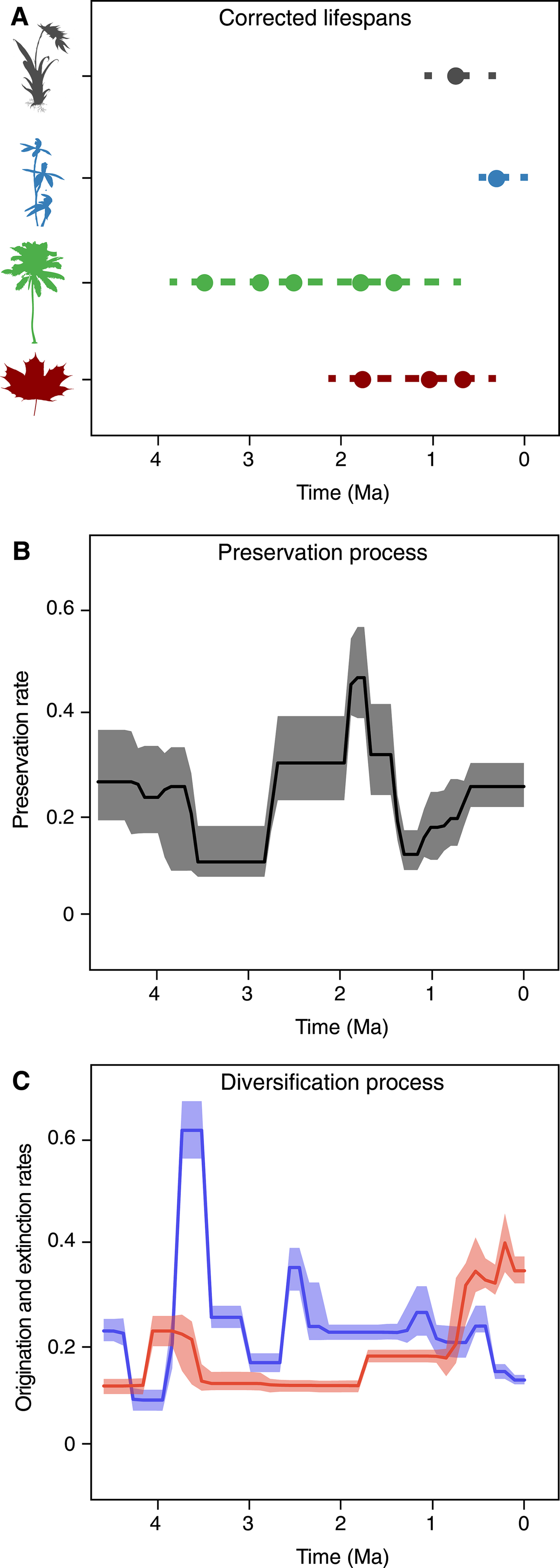
Figure 1. PyRate's main analytical structure. The input data consist of dated fossil occurrences assigned to lineages, e.g., species or genera (represented by circles in A), including singletons and extant taxa. The Bayesian framework jointly estimates the life spans of all lineages (dashed lines), preservation rates (B), and origination and extinction rates (C). All parameter estimates are inferred as posterior mean values (solid lines in B and C) and 95% credible intervals (shaded areas in B and C).
The complexity of this Bayesian probabilistic framework compared with alternative methods (e.g., Foote Reference Foote2001; Alroy Reference Alroy2014; Liow and Finarelli Reference Liow and Finarelli2014) means that a PyRate analysis will typically require a computation time that is longer than that required by other methods by orders of magnitude. While recent studies have compared the performance of these alternative methods using simulated data sets (Smiley Reference Smiley2018), it remains unclear whether PyRate's additional computational burden does in fact return an improved accuracy in the estimated rates of origination and extinction.
One of the main and most challenging aims of the PyRate method is the estimation of how origination and extinction rates vary through time, which is done using a birth–death MCMC (BDMCMC) algorithm (Silvestro et al. Reference Silvestro, Schnitzler, Li, Antonelli and Salamin2014b) to sample the number and temporal placement of rate shifts in a single analysis. The power of this algorithm, however, becomes limited with increasing levels of rate heterogeneity through time and with large data sets (Silvestro et al. Reference Silvestro, Schnitzler, Li, Antonelli and Salamin2014b), thus making the method potentially unsuitable to analyze complex evolutionary histories. Another limitation of the method is that model testing is focused on finding the best birth–death model, while the choice between different preservation models (e.g., with homogeneous or nonhomogeneous rates) remains somewhat arbitrary (e.g., Silvestro et al. Reference Silvestro, Cascales-Miñana, Bacon and Antonelli2015b).
Here, building upon the PyRate platform, we develop novel features that expand the scope and applicability of the program, providing novel models of fossil preservation and improved algorithms. Specifically we (1) introduce more realistic preservation models that simultaneously allow rate heterogeneity across lineages and through time and develop a maximum-likelihood framework to statistically choose the preservation model that best fits the data. (2) We present a more powerful algorithm to infer temporal variation in origination and extinction rates using reversible jump MCMC (RJMCMC; a Bayesian algorithm that jointly infers the number of rate shifts best explaining the data and the parameter values [Green Reference Green1995]) and compare its performance with the alternative BDMCMC algorithm, demonstrating improved results on simulated data. (3) We compare the performance of PyRate against two alternative approaches, the boundary-crossing method (Foote Reference Foote2003) and the three-timer method (Alroy Reference Alroy2014). We analyze simulated data sets generated under different origination and extinction scenarios and compare the accuracy across estimates. (4) We demonstrate some of the novel features developed here with a worked example by analyzing a recently published data set of marine mammals (Pimiento et al. Reference Pimiento, Griffin, Clements, Silvestro, Varela, Uhen and Jaramillo2017) and provide extensive tutorials with detailed descriptions of analysis setup and output processing. (5) Finally, we develop a C++ library which is integrated in the PyRate program and speeds up the analyses by orders of magnitude, thus extending the applicability of the method to very large data sets.
Methods
PyRate implements a hierarchical Bayesian model that jointly samples the preservation rates (indicated by q), the times of origination and extinction for each sampled lineage (indicated by vectors s, e), and the origination and extinction rates (indicated by λ and μ). The input data are fossil occurrences characterized by their ages and their assignment to a taxonomic unit (e.g., a genus or a species) and the origination and extinction rates scaled to the taxonomic unit used in the input data.
The joint posterior distribution of all parameters is approximated by an MCMC algorithm and can be written as
 $$\eqalign{&\underbrace{{P(q,{\bf s},{\bf e},{\rm {\rm \lambda}}, {\rm \mu} \vert X)}}_{{{\rm posterior}}}\propto \underbrace{{P(X \vert q,{\bf s},{\bf e})}}_{{{\rm likelihood}}}{\rm \times} \underbrace{{P({\bf s}{\rm,} {\bf e} \vert {\rm {\rm \lambda}}, {\rm \mu} )}}_{{{\rm birth\hbox{-}death prior}}}\cr & {\rm \times} \underbrace{{P\lpar q \rpar P\lpar {{\rm {\rm \lambda}}, {\rm \mu}} \rpar }}_{{{\rm other (hyper\hbox{-})priors}}}}$$
where  $X = \lcub {{\bf x}_1, \ldots {\bf x}_N} \rcub $ is the list of vectors of fossil occurrences for each of N lineages, so that ${\bf x}_{\bf i} = \lcub {x_1, \ldots, x_K} \rcub $ is a vector of all fossil occurrences sampled for taxon i. The main parameters and models described in this and the following sections are listed in Table 1. We consider here as a fossil occurrence the presence of a species at a sampling locality. The likelihood component of the model allows us to estimate the preservation rates and the times of origin and extinction given the occurrence data, based on a stochastic model of fossilization and sampling (see Preservation Models). The birth–death (BD) prior allows us to infer the underlying diversification process based on the (estimated) origination and extinction times. Additional priors on q, λ, μ enable the estimation of these parameters from the data. The two main components of the PyRate model are sampling (which results from fossil preservation and sampling efforts) and diversification (origination and extinction). Both components are modeled through stochastic processes (as described in the following sections) and estimated in a single analysis.
Table 1. Glossary defining the main terms, acronyms, and parameters used in this study.

Preservation Models
We model the process of fossil preservation and sampling using Poisson processes, wherein the estimated preservation rate(s) indicate the expected number of fossil occurrences per sampled lineage per time unit. Thus, fossil preservation is modeled as a time-continuous stochastic process capturing fossilization, sampling, and identification, that is, all the events occurring from the living organism to the digitized fossil occurrence. The likelihood of a lineage with fossil occurrences x = {x 1, …, x K} given origination time s, extinction time e, and preservation rate q under a general Poisson model is
 $$P({\bf x} \vert q,s,e) = \displaystyle{{{\rm exp}\; \left( {-\int_s^e {q\lpar t \rpar dt}} \right) \times \prod\limits_{i = 1}^K {q\lpar {x_i} \rpar }} \over {K! \times \left( {1-{\rm exp}\; \left( {-\int_s^e {q\lpar t \rpar dt}} \right)} \right)}}$$
where q(t) is the preservation rate at time t (Silvestro et al. Reference Silvestro, Schnitzler, Li, Antonelli and Salamin2014b). The two terms of the numerator quantify the probability of the waiting times between fossil occurrences and the probability of each occurrence. The denominator includes the normalizing constant of the Poisson distribution and the condition on sampling at least one fossil occurrence, where exp (·) represents the probability of zero fossil occurrences between origination and extinction times (Silvestro et al. Reference Silvestro, Schnitzler, Li, Antonelli and Salamin2014b).
The original PyRate implementation included two models of preservation: the homogeneous Poisson process (HPP) and the nonhomogeneous Poisson process (NHPP). The HPP model assumes that the preservation rate is constant throughout the life span of an organism and across time. The NHPP assumes that preservation rates change along the life span of a lineage according to a bell-shaped distribution, in which the rates are lower at the two extremities (i.e., close to the times of origin and extinction of the lineage) and highest in the middle (Silvestro et al. Reference Silvestro, Schnitzler, Li, Antonelli and Salamin2014b). The shape of the distribution is fixed, and the estimated preservation rate q represents the expected number of fossil occurrences per sampled lineage per million years averaged across the life span of the lineage. This model is justified by the empirical observation that the number of occurrences per time unit for a given organism tends to increase following its origination and to decrease before its extinction (Liow et al. Reference Liow, Skaug, Ergon and Schweder2010b). The pattern also reflects the idea that a species originates from a small initial pool of individuals in a restricted geographic area (therefore with lower potential for preservation and sampling) and later expands, thus increasing its chances of leaving a fossil record. Similarly, under this model, species are expected to decline in abundance and geographic range before their extinction (Raia et al. Reference Raia, Carotenuto, Mondanaro, Castiglione, Passaro, Saggese, Melchionna, Serio, Alessio, Silvestro and Fortelius2016), resulting in decreased preservation rates.
Both HPP and NHPP models can be coupled with a gamma model (i.e., HPP + G and NHPP + G), which allows us to incorporate rate heterogeneity across lineages. Under these models, preservation rates are defined so that their mean equals q and their heterogeneity is distributed according to a gamma distribution, with shape parameter α, discretized in a user-defined number of categories (Yang Reference Yang1994; Silvestro et al. Reference Silvestro, Schnitzler, Li, Antonelli and Salamin2014b). The rate parameter of the gamma distribution is set equal to the shape, so the distribution has mean equal to 1. Both q and α are estimated as free parameters by the MCMC, and small values of α indicate increased amounts of heterogeneity. Gamma models do not assign individual preservation rates to each lineage in the data set. Instead, the likelihood of each lineage is averaged across all rates, thus incorporating rate heterogeneity across lineages while adding a single additional parameter (α) to the model (Yang Reference Yang1994).
Here, we introduce a third preservation model that implements a time-variable Poisson process (TPP). The TPP model is an extension of the HPP, in which the rate of preservation is constant within predefined time windows but allowed to change between them. For instance, different preservation rates can be estimated within geological epochs (Foote Reference Foote2001; Liow and Nichols Reference Liow, Nichols, Hunt and Alroy2010). The likelihood of this process is the product of piecewise HPP likelihoods across multiple time frames, each with its specific preservation rate (q = {q 1, …, q W}, where W is the number of time windows in the model). As for the HPP and NHPP models, the TPP can be coupled with a gamma model, therefore allowing for rate heterogeneity both through time and across lineages.
The default prior specified for q is a gamma distribution, chosen to reflect the fact that preservation rates must take positive and real values. Defining appropriate prior distributions is often a challenge in Bayesian analysis, and prior choice can strongly affect the effective parameter space and the complexity of a model (Gelman et al. Reference Gelman, Carlin, Stern and Rubin2013). This may become even more problematic under the TPP model, in which very strict priors could artificially reduce rate heterogeneity through time, whereas very vague priors could unnecessarily expand the amount of parameter space, increasing the risk of overparameterization. To overcome this issue, we use a hyper-prior to estimate the prior on the preservation rates from the data, instead of setting the prior to a fixed distribution. We set a single gamma distribution as prior on the preservation rates q, with a fixed shape parameter (α = 1.5) and unknown rate parameter β. The rate parameter is assigned a vague gamma hyper-prior, β ~ Γ(a = 1.01, b = 0.1), and is itself estimated by the MCMC. Estimating the rate using a hyper-prior makes the gamma prior on q more adaptable to different data sets and reduces the subjectivity of prior choices. Using the properties of the conjugate gamma prior, whereby the posterior distribution of the rate parameter of a gamma likelihood with known shape and gamma-distributed prior is itself a gamma distribution (Gelman et al. Reference Gelman, Carlin, Stern and Rubin2013), we can sample the rate parameter β directly from its posterior distribution, given any vector of preservation rates q, the shape parameter α, and shape and rate of the prior a, b:
 $$P({\rm \beta} \vert {\bf q},{\rm \alpha}, a,b)\sim {\rm \Gamma} \left( {a + {\rm \alpha} W,b + \sum\limits_{i = 1}^W {(q_i)}} \right).$$
A Maximum-Likelihood Test to Compare Preservation Models
Because the preservation process represents a fundamental component of the PyRate model (Fig. 1A,B), it is important to choose the model that best fits the data when analyzing a fossil data set. To this end, we developed a likelihood-based test to assess the statistical fit of alternative preservation processes. The preservation process, with constant or variable rates, is expected to leave a signature in the temporal distribution of fossil occurrences, which will tend to be roughly uniformly distributed under an HPP model (Fig. 2A), to show higher density of record toward the center of a species’ life span under the NHPP model (Fig. 2B) and to follow time-variable distributions under the TPP model (Fig. 2C).
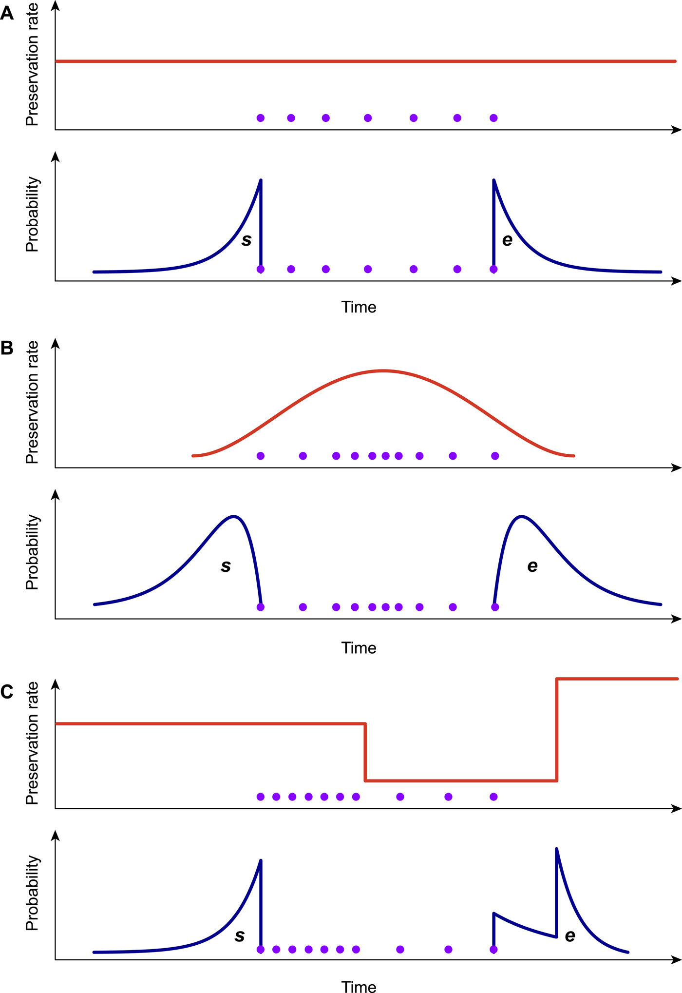
Figure 2. Graphical representation of the preservation rate models implemented in PyRate. In the homogeneous Poisson process model (A), the preservation rate is constant through time, and the expected times of origination and extinction (s, e) are exponentially distributed. In the nonhomogeneous Poisson process model (B), preservation rates vary throughout the life span of a species, generating gamma-like expected s, e. The time-variable Poisson process model (C) assumes piecewise constant preservation rates (e.g., different rates for each epoch) and the resulting expected s, e values combine multiple exponential distributions. All models can incorporate rate heterogeneity across lineages (gamma models).
Although it is theoretically possible to infer the marginal likelihood of a preservation model in a Bayesian framework (for instance using the thermodynamic integration available in PyRate to test between alternative birth–death models [Lartillot and Philippe Reference Lartillot and Philippe2006; Silvestro et al. Reference Silvestro, Schnitzler, Li, Antonelli and Salamin2014b]), the task would be computationally extremely demanding. Indeed, the number of parameters over which the likelihood needs to be marginalized can be very high, including the vectors of origination and extinction times, the preservation rates, and potentially the parameters of the birth–death prior. Thus, we implemented a maximum-likelihood test for preservation models that substantially reduces the computational burden. This maximum-likelihood test is intended as a first step in the analysis of a fossil data set, in which the best preservation model is identified. Then, the full Bayesian analysis of preservation, origination, and extinction rates is performed under the selected preservation model (see also Analysis Protocol for Marine Mammals, Supplementary Material).
Let  $\hat{s}$ and $\hat{e}$ be the expected times of origination and extinction of a lineage with fossil occurrences ${\bf x} = \lcub {x_1, \ldots, x_K} \rcub $ (sorted from oldest to most recent) for a given preservation rate q. To compare the fit of different models, we maximize the likelihood $P({\bf x},\hat{s},\hat{e}\vert q)$, where q is treated as a free parameter and estimated in the optimization, while $\hat{s}$ and $\hat{e}$ are calculated based on the preservation rate and model. In the simplest case of an HPP of preservation, the expected times of origination and extinction are determined by the expectation of an exponential distribution with rate equal q: E[Exp(q)] = 1/q. Thus, under HPP, the expected times of origination and extinction are $\hat{s} = x_1 + 1/q$ and $\hat{e} = x_K-1/q$ (Fig. 2A). Note that the expected times of origination and extinction differ from their maximum-likelihood estimates, which under HPP are s ML = x 1 and e ML = x K.
In the case of the NHPP model, neither the expectation nor the maximum-likelihood values of s and e are easily derived analytically. Instead, we use a two-step approach to obtain a maximum-likelihood value that is comparable to that obtained under HPP. First, we optimize the rate q by maximizing the likelihood P(x|q, s, e), where q, s, and e are treated as free parameters. This results in maximum-likelihood estimates of the preservation rate (q ML) and origination and extinction times (s ML and e ML). Second, because the likelihoods of different preservation models are compared based on the expected origination and extinction times (i.e., not their maximum-likelihood values), we use MCMC sampling to infer  $\hat{s}$ and $\hat{e}$, given the estimated rate q ML (Fig. 2B). The MCMC samples from the posterior probability
 $$P(s,e \vert q_{{\rm ML}},{\bf x})\propto P({\bf x} \vert q_{{\rm ML}},s,e) \times P(s)\; P(e)$$
where  $P\lpar s \rpar \sim {\rm {\cal U}}\lpar {x_1,\infty} \rpar $ and $P\lpar e \rpar \sim {\rm {\cal U}}\lpar {0,x_K} \rpar $ are uniform priors on origination and extinction times. These priors, while unrealistic, essentially imply that the acceptance probability of the MCMC is only driven by the likelihood surface. We sample 1000 values of s and e and use their mean as expected origination and extinction times $\hat{s}_q$, and $\hat{e}_q$. Once we have obtained $\hat{q}$, $\hat{s}_q$, and $\hat{e}_q$, we can calculate the likelihood of the data given the model and use it for model comparison.
Under the TPP model, the expected times of origination and extinction are determined by a combination of exponential expectations with rate parameters (i.e., preservation rates) q = {q 1, …, q W}, truncated at the boundaries of each of W time window (Fig. 2C). For any given preservation rate q, we use numerical integration to approximate the resulting distribution and obtain expected values for the times of origination and extinction  $(\hat{s},\hat{e})$. We use maximum likelihood to optimize the vector of preservation rates.
The likelihood of a data set encompassing multiple taxa, under any preservation model, is the product of the individual likelihood of each lineage (Silvestro et al. Reference Silvestro, Schnitzler, Li, Antonelli and Salamin2014b). For the purpose of model testing between HPP, NHPP, and TPP models, we assume that the preservation rates are constant across lineages and therefore optimize a single parameter q (or vector of parameters q under the TPP model) to obtain the maximum likelihood of the data. We then calculate the fit of each model using the Akaike information criterion corrected for sample size (AICc), based on the number of analyzed lineages (Burnham and Anderson Reference Burnham and Anderson2002). We consider this test as a useful tool to choose between qualitatively different preservation processes (HPP, NHPP, and TPP) and advise researchers to always couple the best-fitting Poisson process with the gamma model in empirical analyses. The risk that the gamma model represents an overparameterization of the preservation process is minimal, because the gamma model only adds a single parameter to incorporate any potential amount of rate heterogeneity across clades (Silvestro et al. Reference Silvestro, Schnitzler, Li, Antonelli and Salamin2014b). Additionally, virtually all empirical data sets we have analyzed so far indicated very high levels of rate variation across clades (see also “Results”).
AICc Thresholds and Testing
We used simulated data to assess the performance of our likelihood test for preservation models. We simulated 1000 data sets of fossil occurrences under each of three models (HPP, NHPP, and TPP). Each simulation included 100 lineages, with life span determined by a randomly sampled extinction rate  ${\rm \mu} \sim {\rm {\cal U}}\lsqb {0.05,0.5} \rsqb $, reflecting a realistic range of extinction rates (Pimiento et al. Reference Pimiento, Griffin, Clements, Silvestro, Varela, Uhen and Jaramillo2017). Thus, for the properties of the birth–death process (Kendall Reference Kendall1948), the distribution of life spans followed an exponential distribution with mean 1/μ. Fossil occurrences were then simulated based on each Poisson process with a rate q randomly drawn from ${\rm {\cal U}}\lsqb {0.05,3.5} \rsqb $. The rate q represented the mean preservation rate for each lineage in NHPP simulations (Silvestro et al. Reference Silvestro, Schnitzler, Li, Antonelli and Salamin2014b). In TPP simulations, we simulated one shift in preservation rate occurring halfway between the origination time of the oldest lineage and the most recent extinction time. The preservation rate after the shift was then set to 5 × q.
Although singletons (i.e., lineages represented by a single fossil occurrence) can be analyzed and are usually included in PyRate analyses, they should be removed when the aim to compare the fit of different preservation models. While singletons contribute to the correct inference of preservation rates in an analysis aimed at parameter estimation, at least one waiting time between occurrences is needed when testing among preservation models. Singletons are therefore removed automatically from the data when using the model-testing function implemented in PyRate. Thus, before running the test on simulated data, we removed all lineages with fewer than 2 occurrences. This procedure left, depending on the simulation settings, between 10 and 100 sampled lineages, providing a range of data sizes.
We used simulations to define the appropriate ΔAICc thresholds necessary to confidently choose between preservation models. While the model yielding the smallest AIC score can be considered as best fitting (Burnham and Anderson Reference Burnham and Anderson2002), small differences in AICc values might be difficult to interpret, and the threshold for significance is often obtained through simulations (e.g., Dib et al. Reference Dib, Silvestro and Salamin2014; Pennell et al. Reference Pennell, Eastman, Slater, Brown, Uyeda, FitzJohn, Alfaro and Harmon2014). Additionally, empirically verifying the accuracy of model testing is especially important here, because the optimization involves a combination of analytical expectations of origination and extinction times for HPP and numerical approximations for NHPP and TPP. Thus, we used the 3000 simulations (for which the true generating model is known) as a training set and for each computed AICc score under the three preservation models. Based on the resulting distributions of AICc scores, we determined the ΔAICc thresholds that yielded less than 5% errors and less than 1% errors in model selection. We then simulated an additional 300 data sets (100 for each preservation model) to verify the appropriateness of the thresholds (Supplementary Figs. S1–S3).
Time-Variable Birth–Death Models
The temporal distribution of origination and extinction times of sampled lineages, estimated through the preservation process, is modeled to be the result of a time-continuous birth–death stochastic process, in which lineages originate at a rate λ and go extinct at a rate μ (Kendall Reference Kendall1948). PyRate implements several birth–death models, in which rates can change through time at discrete events or rate shifts (Silvestro et al. Reference Silvestro, Schnitzler, Li, Antonelli and Salamin2014b), following time-continuous variables (Lehtonen et al. Reference Lehtonen, Silvestro, Karger, Scotese, Tuomisto, Kessler, Peña, Wahlberg and Antonelli2017). The general likelihood of a birth–death process with time-variable rates is derived from Keiding (Reference Keiding1975):
 $$\eqalign{&P({\bf s},{\bf e} \vert {\rm {\rm \lambda}}, {\rm \mu} )\propto \mathop \prod \limits_{i = 1}^N {\rm {\rm \lambda}} \lpar {s_i} \rpar \times {\rm \mu} (e_i)^{I_i} \cr & \times \exp {\rm \;} \left( {-\int_{s_i}^{e_i} {{\rm {\rm \lambda} (}t{\rm )} + {\rm \mu} (t)\; dt}} \right)}$$
where N is the number of lineages, λ(t) is the origination rate at time t, μ(t) is the extinction rate at time t, and I i is an indicator set to I i = 1 if species i is extinct (e i >0) and I i = 0 if species i is extant (in which case the extinction time e i = 0 is not sampled as a parameter).
A birth–death model with rate shifts (BDS) is characterized by changes in rates of origination and extinction at shift times, while the rates are constant between shifts (Silvestro et al. Reference Silvestro, Schnitzler, Li, Antonelli and Salamin2014b). The BDS model is described by a vector of origination rates Λ = {λ0, λ1, …, λJ} delimited by times of shifts  ${\rm \tau} ^{\rm \Lambda} = \lcub {{\rm \tau}_1^{\rm \Lambda}, \ldots, {\rm \tau}_J^{\rm \Lambda}} \rcub $ and by extinction rates M = {μ0, μ1, …, μH} delimited by times of shifts ${\rm \tau}{}\hskip1pt^M = \lcub {{\rm \tau}_1^{M}, \ldots, {\rm \tau}_H^M} \rcub $, where J and H represent the number of origination and extinction rate shifts, respectively. Under this notation, origination and extinction rates are constant and equal to λ0 and μ0, respectively, when the model includes no rate shifts. The original PyRate implementation used a Bayesian algorithm, the BDMCMC (Stephens Reference Stephens2000), to jointly infer the number of rate shifts ( J and H), the rates between shifts (Λ, M), and the times of rate shift (τΛ, τM). While we showed BDMCMC to be able to correctly infer rate variation under several scenarios, it tends to be too conservative in assessing rate heterogeneity through time when the true generating process involves several rate shifts (Silvestro et al. Reference Silvestro, Schnitzler, Li, Antonelli and Salamin2014b). In the following sections we develop an alternative method to estimate birth–death models with rate shifts using the more general RJMCMC algorithm (Green Reference Green1995) and demonstrate through simulations that it outperforms BDMCMC.
Inferring Rate Variation Using RJMCMC
The RJMCMC algorithm is a modified version of the standard Metropolis-Hastings MCMC, in which the model (here the number of rate shifts) is itself considered a parameter. In a maximum-likelihood framework, model testing is typically done using AIC or similar metrics that penalize parameter-rich models to find the best balance between model fit and its complexity. The RJMCMC algorithm “jumps” across different models and uses the posterior ratio to avoid under- and overparameterization. The result of RJMCMC is a posterior sample of parameter values (here origination and extinction rates through time) averaged over model uncertainty and posterior probabilities associated with each model, while incorporating the uncertainties associated with the preservation process.
In the RJMCMC framework, the number of rate shifts is considered an unknown variable and is estimated from the data. To this end we include two additional types of proposals: namely, the forward move and the backward move, which add or remove rate shifts, respectively, thus changing the number of parameters in the birth–death model. Given that these moves are identical for both speciation and extinction rates, we use the notation Φ to denote either the speciation (Λ) or extinction (M) rates. We indicate the time frames identified by rate shifts with Δ = {δ0, δ1, …, δK−1}. Under this notation, we set δi = τi − τi+1, where τ is the time of rate shift for 0 < i ≤ K, whereas  ${\rm \tau} _0 = \max ({\bf s})$ and ${\rm \tau} _{K + 1} = \min ({\bf e})$ represent the maximum and minimum ages, respectively, of the full birth–death process spanned by the data. A given set of time frames Δ of length K is associated with a vector of rate parameters Φ = {ϕ0, ϕ1, …, ϕK}.
The RJMCMC algorithm requires a modification in the acceptance rule of a standard MCMC in order to maintain its reversibility while moving across models with different parameterizations (Green Reference Green1995). The general form of the acceptance probability for a forward move (i.e., adding a rate shift) can be written as min{1, A(θ, θ′)}, where θ and θ′ are the model parameters of the current and new states, respectively, and A(θ, θ′) is the product of three main terms:
 $$\eqalign{A\lpar {{\rm \theta}, {{\rm \theta}}^{\prime}} \rpar & = \underbrace{{\displaystyle{{{\rm \pi} \lpar {{{\rm \theta}}^{\prime}} \rpar } \over {{\rm \pi} \lpar {\rm \theta} \rpar }}}}_{{{\rm Posterior}\;{\rm ratio}}}{\rm \times} \underbrace{{\displaystyle{{P({\rm {\cal M}} \vert {\rm {{\cal M}}^{\prime}})} \over {P({\rm {{\cal M}}^{\prime}} \vert {\rm {\cal M}})}} \times \displaystyle{{P({\rm \theta} \vert {{\rm \theta}} ^{\prime})} \over {P({{\rm \theta}} ^{\prime} \vert {\rm \theta} )}}}}_{{{\rm Hastings}\;{\rm ratio}}} \cr & {\rm \times} \underbrace{{\left \vert {\displaystyle{{\partial \lpar {{{\rm \theta}}^{\prime}} \rpar } \over {\partial \lpar {{\rm \theta}, u} \rpar }}} \right \vert}} _{{{\rm Jacobian}}}}$$
The first term is the posterior ratio, that is, the ratio between unnormalized posterior probabilities, of the new state over the current state (where π(·) indicates the posterior as in eq. 1). The second term, often referred to as the Hastings ratio (e.g., Heath et al. Reference Heath, Hulsenbeck and Stadler2014), describes the ratio between the probability of going back from the new state to the current one and the probability of proposing the new state given the current one. This term includes the probability of a forward move, which generates a new model  ${\rm {{\cal M}}^{\prime}}$ from the current one ${\rm {\cal M}}$ by adding a rate shift and the probability of a backward move, which removes a rate shift. The Hastings ratio also includes the probability of proposing a new parameter state θ′ from the current one θ and vice versa. Note that the new and current states will differ in the number of parameters by one additional time of rate shift and one additional rate shift. The third term is the Jacobian of the deterministic function mapping the values of the parameters of the current state into the parameters of the new state and corrects for the change in the dimensionality of the parameter space. The acceptance probability of a backward move (i.e., removing a rate shift) can be directly deduced from the associated forward move. The move from a model with parameters θ (with K rates) to a model θ′ (with K − 1 rates) has the acceptance probability set to min[1, A(θ′, θ)], with
 $$A\lpar {{{\rm \theta}}^{\prime},{\rm \theta}} \rpar = A({\rm \theta}, {{\rm \theta}} ^{\prime})^{-1}.$$
Probability of a Reversible Jump
In our implementation, forward and backward moves are selected with equal probability  $P({\rm {\cal M}}_{K + 1}\vert {\rm {\cal M}}_K) = P({\rm {\cal M}}_K\vert {\rm {\cal M}}_{K + 1}) = 0.5$, except for the boundary cases K = 1 and K = K max, where K max is the maximum allowed number of rate shifts. When K = 1, that is, constant rates and no rate shift, forward moves are proposed with probability 1, while only backward moves are proposed when K = K max. To avoid numerical issues (e.g., overflows), PyRate does not allow time windows smaller than 1 time unit (i.e., δ ≥ 1), therefore resulting in K max = τK+1 − τ0.
Forward Move: Adding a New Rate Shift
A forward move from model  ${\rm {\cal M}}_K$ to ${\rm {\cal M}}_{K + 1}$ is done by splitting an existing time frame into two time frames to which new rates are assigned. We first select a time frame δi randomly from Δ and split it into two time frames δx, δy by drawing a new time of rate shift τ′ from ${\rm {\cal U}}\lpar {{\rm \tau}_i,{\rm \tau}_{i + 1}} \rpar $. Because δx + δy = δi, we can calculate the relative weight of the two new time frames as w x = δx/δi and w y = δy/δi. We then assign the rates ϕx and ϕy to the new time frames to replace the original ϕi. Although the new rates could be drawn from independent distributions, we choose ϕx and ϕy, such that their weighted geometric mean equals the original rate ϕi, which was shown to be more efficient in Poisson processes with rate shifts Green (Reference Green1995). The weights are w x and w y (i.e., based on the relative size of the new time frames) and the new rates are chosen so that
 $${\rm \phi} _i = \exp \lsqb {w_x\log ({\rm \phi}_x) + w_y\log ({\rm \phi}_y)} \rsqb $$
We draw a random variable u from a beta distribution  ${\cal B}\lpar {{\rm \alpha}, {\rm \beta}} \rpar $ that quantifies the amount of discrepancy between rates ϕx and ϕy by using the following equation
 $$\displaystyle{{1-u} \over u} = \displaystyle{{{\rm \phi} _y} \over {{\rm \phi} _x}}.$$
We therefore generate the new rates as:
 $${\rm \phi} _x = \exp \lcub {\log \,({\rm \phi}_i)-w_y\log \lsqb {\lpar {1-u} \rpar /u} \rsqb } \rcub $$
 $${\rm \phi} _y = \exp \lcub {\log({\rm \phi}_i) + w_x\log \lsqb {\lpar {1-u} \rpar /u} \rsqb } \rcub $$
The parameters of the beta distribution are set by default to α = β = 10, yielding an expected E[u] = 0.5, with 95% of the values ranging from 0.29 to 0.71. We chose these values as they provided good convergence in our tests, although PyRate includes commands to easily tweak this and other tuning settings.
The Hastings ratio for a forward move M k → M k+1 is computed as
 $$\eqalign{& \displaystyle{{P({\rm {\cal M}} \vert {\rm {{\cal M}}^{\prime}})} \over {P({\rm {{\cal M}}^{\prime}} \vert {\rm {\cal M}})}} \times \displaystyle{{{(K + 1)}^{-1}} \over {{(K + 1)}^{-1}}} \times \displaystyle{1 \over {P(u \vert {\rm \alpha}, {\rm \beta} )}} \cr & \quad \times \displaystyle{1 \over {{({\rm \delta} _i)}^{-1}}},}$$
where the first ratio is based on the simple rules described earlier and allows forward and backward moves with equal probabilities when 1 < K < K max. The numerator and denominator of the second ratio define the uniform probability of drawing one of the K rate shifts from the new model  ${\rm {\cal M}}_{K + 1}$ and the uniform probability of drawing one of the K time frames from the current model ${\rm {\cal M}}_K$, respectively (noting that a model with K rate shifts includes K + 1 time frames). The two following denominators identify the probability of drawing u from its distribution β(α, β), where P(u|α, β) is based on the probability density function of a beta distribution and the probability of uniformly drawing a new rate shift within time frame δi. The Jacobian for the transformation of variables (ϕi, u) → (ϕx, ϕy) (eq. 9) is equal to (Green Reference Green1995):
 $$\displaystyle{{\partial \lpar {{\rm \phi}_x,{\rm \phi}_y} \rpar } \over {\partial \lpar {{\rm \phi}_i,u} \rpar }} = \displaystyle{{{({\rm \phi} _x + {\rm \phi} _y)}^2} \over {{\rm \phi} _i}}.$$
Backward Move: Removing an Existing Rate Shift
A backward move from model  ${\rm {\cal M}}_{K + 1}$ to ${\rm {\cal M}}_K$ is done by removing an existing rate shift and merging the two adjacent time frames and their rates. The first step is to randomly select a rate shift J over the K − 1 existing ones. The temporal placement of the rate shift is τj, and its adjacent time frames are identified as δj−1 and δj. Thus, the rates ϕx and ϕy are combined to obtain a new rate ϕi based on equation (8).
For a backward move  ${\rm {\cal M}}_{K + 1}\to {\rm {\cal M}}_K$, the same computations are applied, but the Hastings ratio and the Jacobian must be inverted as defined in equation (7). The value u must be defined using equation (9) in order to compute P(u|α, β).
Priors on the Number of Shifts
Because the number of origination and extinction rates (J and K, respectively) are considered unknown variables in the RJMCMC implementation, we assign them a prior distribution to sample them from their posterior distribution. We use a single Poisson distribution with rate parameter r to compute the prior probability of J and K. To reduce the subjectivity of the prior, we consider r itself an unknown parameter and estimate it from the data. We assign a gamma hyper-prior, which allows us to sample r directly from its conjugate posterior distribution for any given J and K values:
 $$P(r \vert J,K,{\rm \alpha}, {\rm \beta} )\sim {\rm \Gamma} \lpar {{\rm \alpha} + J + K,\; b + 2} \rpar,$$
where α and β are the shape and rate parameters of the gamma hyper-prior distribution. In our simulations, we use the hyper-prior Γ(α = 2, β = 1), which sets the highest prior probability to models with constant origination and extinction rates (i.e., mode = 1).
Marginal Origination and Extinction Rates
To summarize the origination and extinction rates sampled by RJMCMC, we marginalize them within arbitrary small (user-defined) time bins. We emphasize that this procedure does not imply that the birth–death process itself is discretized in time bins, as both the origination and extinction events are modeled within a time-continuous stochastic process. The marginal distributions of origination and extinction rates incorporate uncertainties on: (1) the true times of origination and extinction of sampled lineages, which are themselves a function of the preservation process; (2) the number of rate shifts as sampled by the RJMCMC; and (3) the temporal placement of the rate shifts. We summarize the marginal rates by computing their posterior mean and 95% credible intervals (95% CI).
Timing of Significant Rate Shifts
We implemented a function to assess the timing of significant rate changes based on the RJMCMC posterior samples. To this end, we compute the frequency of sampling a rate shift (using arbitrarily small time bins) and plot them against time to assess when rate shifts are more likely to have occurred. To assess whether the frequency of a rate shift significantly exceeds the prior expectation, we run an MCMC simulation in which the number and times of rate shifts are purely sampled from their respective priors, that is, a uniform distribution on the times of shift and Poisson distributions on the number of speciation and extinction rates with a gamma prior assigned to its hyper-parameter r (see previous paragraph). From the samples obtained from the simulation, we compute the prior probability of a rate shift at any given time, based on the user-specified size of the bins.
We then compute the posterior sampling frequencies corresponding to significant statistical support based on the standard log Bayes factors thresholds (so that 2log BF = 2 and 6, for positive and strong support, respectively) (Kass and Raftery Reference Kass and Raftery1995).
Given the two alternative hypotheses (presence or absence of a shift in a bin), we can define the Bayes factor as the posterior odds divided by the prior odds (Kass and Raftery Reference Kass and Raftery1995):
 $${\rm BF} = \displaystyle{{P({\rm \tau} \vert D)} \over {1-P({\rm \tau} \vert D)}}/\displaystyle{{P\lpar {\rm \tau} \rpar } \over {1-P\lpar {\rm \tau} \rpar }},$$
where P(τ|D) is the posterior probability of a rate shift, and P(τ) is its prior probability. After solving the equation for the posterior term, we obtain that the posterior probability corresponding to a 2log BF = x is
 $$\eqalign{P({\rm \tau} \vert D) & = \displaystyle{A \over {1 + A}},\;{\rm where}\;A \cr & = \exp {\rm \;} \left( {\displaystyle{x \over 2}} \right)\displaystyle{{P\lpar {\rm \tau} \rpar } \over {1-P\lpar {\rm \tau} \rpar }}.}$$
We implemented these calculations directly into a single function that generates plots of marginal origination and extinction rates through time and posterior frequencies of rate shifts through time, with dashed lines indicating positive and strong statistical support based on Bayes factors (i.e., 2 log BF = 2 and 6, respectively [Kass and Raftery Reference Kass and Raftery1995]).
Validation of the Method through Simulations
We tested the new RJMCMC algorithm on simulated data sets and compared its performance with that of the BDMCMC algorithm previously implemented in PyRate. We simulated fossil data sets under three different birth–death scenarios:
1. Constant origination and extinction rates set to 0.15 and 0.07, respectively, with root age set to 45 Ma.
2. Time-variable birth–death model with 2 rate shifts in origination and 2 rate shifts in extinction. The time of origin was set to 35, with origination rate shifts at 20 and 10 Ma and extinction rate shifts at 15 and 10 Ma. Origination rates decreased across time windows [Λ = (0.4, 0.1, 0.01)], whereas extinction rates peaked between 15 and 10 Ma [M = (0.05, 0.3, 0.01)].
3. Time-variable birth–death model with 4 rate shifts in origination (at 30, 18, 15, and 7 Ma) and 4 rate shifts in extinction (at 25, 22, 17, and 2). Origin time was set to 45 Ma, and the rates between shifts were: Λ = {0.3, 0.07, 0.6, 0.05, 0.3} and M = {0.02, 0.6, 0.05, 0.2, 0.5}.
We simulated 100 data sets under each scenario, assuming a homogeneous Poisson process of preservation, with rate drawn from a uniform distribution  $q\sim {\rm {\cal U}}\lsqb {0.5,1.5} \rsqb $. To avoid extremely small or large data sets, we constrained the simulations to yield between 150 and 250 lineages. We analyzed each data set using both BDMCMC and RJMCMC, running 2,000,000 MCMC iterations for each algorithm and sampling every 1000 iterations.
We assessed the performance of the BDMCMC and RJMCMC algorithms by quantifying their ability to infer the correct number of rate shifts and the accuracy and precision of the origination and extinction rates, marginalized within 1 Myr time bins. We computed the posterior probability of models with different numbers of rate shifts based on their sampling frequencies and compared them with the true values used to simulate the data. To quantify the accuracy of rate estimates, we used the posterior mean of the marginal rates at different times and calculated the relative error as the absolute difference between the estimated rate (r est) and the true rate (r true) relative to their mean, that is, (|r est − r true|)/[(r true + r est)/2]. Relative errors were then averaged across rates and among simulations. We also summarized the precision of the rate estimates in terms of size of the 95% CI relative to the mean rate, again averaged across rates and among simulations.
Comparisons with Other Approaches
We analyzed the same simulated data sets using two alternative methods to infer origination and extinction rates, the boundary-crossing method (Foote Reference Foote2000) and the three-timer method (Alroy Reference Alroy2015) as implemented in the R package ‘fbdR’ (github.com/rachelwarnock/fbdR). We binned fossil occurrences based on 20 time intervals of equal size (bin size of 1.75–2.25 Myr depending on the simulation) and inferred origination and extinction rates within each bin. Although there exist methods to infer some confidence intervals around rate estimates (Foote Reference Foote2001), these are not necessarily comparable with the 95% credible intervals obtained from Bayesian inferences. Thus, we focused the comparison on the accuracy of the estimates, rather than on their precision (which was only evaluated for the PyRate method; see Validation of the Method through Simulations). We therefore quantified the accuracy of the estimates by computing the relative errors averaged through time as done for the PyRate estimates and compared relative errors among methods.
Empirical Case Study
We demonstrate the new PyRate implementation by analyzing genus-level fossil occurrences of marine mammals recently compiled by Pimiento et al. (Reference Pimiento, Griffin, Clements, Silvestro, Varela, Uhen and Jaramillo2017). The data included 535 genera, 73 of which are extant, and 4740 occurrences spanning from the Eocene to the recent. Because the dating of most fossil occurrences is given as a temporal range, we resampled the age of each occurrence uniformly from its range and produced 10 randomized input files, as in Silvestro et al. (Reference Silvestro, Schnitzler, Li, Antonelli and Salamin2014b). We then repeated all analyses on each replicate and combined the results to incorporate dating uncertainties in our estimates.
First of all, we ran a model test to choose the most appropriate preservation model. We tested the HPP and NHPP models as well as a TPP model with rate shifts set at the boundaries between epochs in the Cenozoic. We therefore ran the subsequent analyses using the best-fitting preservation model and added the gamma option to allow for rate heterogeneity across lineages. We assumed a birth–death process with rate shifts and used the RJMCMC algorithm to determine the number and temporal placement of the shifts and the origination and extinction rates through time. After running 50 million iterations, sampling every 10,000 iterations, we combined samples of the 10 randomized data sets to infer the number of rate shifts and plot origination and extinction rates through time. The complete list of commands used for the empirical analyses presented here along all input files are available as Supplementary Material (Dryad Repository: https://doi.org/10.5061/dryad.j3t420p).
We analyzed the marine mammal data set under the boundary-crossing and three-timer methods, for comparison. The ages of fossil occurrences were randomized 100 times based on the respective stratigraphic intervals, and the rates were estimated across equal time bins of 2 Myr, using the R package ‘divDyn’ (Kocsis et al. Reference Kocsis, Reddin, Alroy and Kiessling2019).
Performance Boost
Because of the large number of parameters estimated in a typical PyRate analysis and due to the inherent iterative nature of MCMC algorithms, the analyses of large fossil data sets (e.g., hundreds or thousands of lineages) can be very time-consuming. We therefore developed a Python module named FastPyRateC to boost the performance of the analysis. This module consists of a SWIG (http://www.swig.org) wrapper to a fast C++ implementation of PyRate core functions such as the main likelihood functions (e.g., preservation models and most available birth–death models). This module is precompiled for the main operating systems (see Software Availability), can be easily compiled using a Python installation script, and requires a single external dependency, the C++ boost library (http://www.boost.org).
We assessed the improvement in performance by running analyses on three data sets of 50, 150, and 300 lineages (with 543, 1368, and 2736 fossil occurrences, respectively). We ran 100,000 RJMCMC iterations under the HPP, NHPP, and TPP models coupled with the gamma model of rate heterogeneity among lineages. Analyses were run on a Macintosh computer with a 3.1 GHz Intel Core i7 processor. We ran with and without the FastPyRateC library to compute the speed-up achieved by the C++ library and estimate the time necessary to run the default 10 million iterations, which are the default number of iterations in PyRate.
Results
Testing among Preservation Models
The maximum-likelihood test implemented to distinguish among alternative preservation processes provides a reliable tool to infer the correct model. Extensive simulations show that different δ AIC thresholds can be applied for different competing models. For instance, if the best model (smallest AIC) is obtained for NHPP, we can reject the HPP model as a valid alternative only if AICHPP-AICNHPP >3.8 (for a 5% error tolerance) or AICHPP-AICNHPP >8 (for a 1% error tolerance). However, the TPP model can be confidently rejected simply based on AICTPP-AICNHPP >0. The full set of thresholds derived from our simulations is given in Table 2 and incorporated in the model test as implemented in PyRate 2.0.
Table 2. Thresholds for change in Akaike information criterion (ΔAICc) estimated by simulations to test between different preservation models. Depending on the selected best model (i.e., the one with the lowest AICc score), different thresholds are applied to determine whether the model is significantly better than the alternatives (p <0.05). Values in parentheses show the thresholds estimated for p <0.01. Cases in which ΔAICc values do not exceed the thresholds provided here indicate that the evidence in the data is not sufficient to confidently choose among preservation models. HPP, homogeneous Poisson process; NHPP, nonhomogeneous Poisson process; TPP, time-variable Poisson process.

Our simulations show that the ability to statistically distinguish between preservation models (computed as δ AIC scores) generally increases with the size of the data set, that is, number of lineages and number of occurrences (Supplementary Figs. S1–S3). Increasing preservation rates also yield stronger support for the correct model. Additionally, there is an effect of the extinction rate, whereby lower extinction rates are associated with better differentiation between preservation models. This effect is likely linked with the increased mean longevity of lineages, which therefore tend to accumulate more occurrences.
Performance of RJMCMC Compared with BDMCMC
The RJMCMC algorithm outperformed the BDMCMC alternative in most simulations (Table 3). The RJMCMC method identified the correct number of shifts in origination rates in 88% of the simulations. In comparison, the BDMCMC method identified the correct model of origination in 52% of the simulations. This value is mostly driven by a consistent underestimation of rate heterogeneity in simulation scenarios 2 and 3. The RJMCMC analyses identified the correct model of extinction in 67% of the simulations. We note that the correct number of shifts in extinction rates was found in 99% of the simulations under scenarios 1 and 2, whereas under scenario 3 the algorithm consistently inferred four rates instead of five, suggesting that one of the rate shifts did not leave a significant signature on the simulated fossil data. The BDMCMC analyses correctly identified the absence of extinction rate shifts in scenario 1, but were substantially less accurate than RJMCMC analyses in finding the correct model in the case of rate heterogeneity (Table 3).
Table 3. Model testing using the reversible jump Markov chain Monte Carlo (RJMCMC ) and birth–death Markov chain Monte Carlo (BDMCMC) algorithms. The simulations (replicated 100 times) are based on different numbers of origination rates (J) and extinction rates : (1) J = 1, K = 1; (2) J = 3, K = 3; and (3) J = 5, K = 5. For each value of J and K , we estimated the how frequently it was estimated as the best model by RJMCMC and BDMCMC across all replicates. Values in bold represent the frequencies at which the correct models were identified by the algorithms.

The marginal rates of origination and extinction were estimated with high accuracy by both BDMCMC and RJMCMC under scenario 1 (constant rates), with relative errors between 0.09 and 0.14 (Table 4, Supplementary Fig. S4). In contrast, simulations based on time-variable origination and extinction rates show that RJMCMC estimates are substantially more accurate than those yielded by BDMCMC (Fig. 3; Supplementary Fig. S5). For instance, for scenario 2, RJMCMC estimates marginal rates with an average relative error around 0.26, about three times more accurate than the rates obtained from BDMCMC. These results reflect the better ability of RJMCMC to recover the correct birth–death model, in terms of number of rate shifts (Table 3).

Figure 3. Marginal rates through time inferred for simulation scenario 2. The data sets were simulated under decreasing rates of origination (with shifts at 20 and 10 Ma) and extinction rates (with a peak at 15–10 Ma; true values are shown as dashed lines). Estimates are averaged across 100 simulations, with the shaded areas showing 95% credible intervals. The top row shows the origination and extinction rates inferred using the birth–death Markov chain Monte Carlo algorithm, whereas the bottom row shows the results of the reversible jump Markov chain Monte Carlo.
Table 4. Comparison of accuracy and precision of the marginal origination and extinction rates between the new reversible jump Markov chain Monte Carlo (RJMCMC ) and birth–death Markov chain Monte Carlo (BDMCMC) algorithms. Accuracy (relative errors) and precision are averaged across analyses of 100 simulated data sets for each simulation scenario. While the precision of rate estimates (here quantified by the relative size of the 95% credible intervals) is similar between algorithms, the RJMCMC implementation yields substantially more accurate results, especially in the presence of rate heterogeneity through time.

Performance of PyRate Compared with Other Methods
Although all methods correctly picked up the general trends in diversification rates, PyRate estimates of both origination and extinction rates through time decisively outperformed the results of the boundary-crossing and three-timer methods under our simulation settings. The accuracy of the estimates was similar between boundary-crossing and three-timer and substantially higher in PyRate estimates (Fig. 4A). The relative errors generally ranged between 50 and 130% when using boundary-crossing and three-timer methods and ranged between 10 and 50% in PyRate estimates.

Figure 4. Origination and extinction rates estimated using different methods. Relative errors (A) in the rate estimates as inferred using the boundary-crossing method (Foote Reference Foote2000), the three-timer approach (Alroy Reference Alroy2014), and our new algorithm implemented in PyRate. Box plots summarize the results of 100 simulations under three diversification scenarios. The errors were computed based on the rate estimates within 2 Myr time bins in boundary-crossing and three-timer analyses and based on the posterior means of the marginal rates through time in PyRate analyses (B).
The difference in accuracy between methods does not appear to stem from any systematic bias in the estimates. Instead, it is mostly linked to a higher volatility of the estimated rates through time under the boundary-crossing and three-timer methods, which is apparent from the rates-through-time plots (Fig. 4B, Supplementary Figs. S6–S8). The volatility of the rate estimates is especially high for simulation scenario 1 (constant rates; Supplementary Fig. S6) and, in general, early in the history of the clade (e.g., the first 10–15 Myr in simulation scenarios 1 and 2; Fig. 4B, Supplementary Fig. S6), where the size of the clade in terms of number of sampled species is lower.
Diversification Dynamics of Cenozoic Marine Mammals
The maximum-likelihood test of preservation models resulted in a very strong support for the TPP model against the HPP (ΔAICc = 324.23) and NHPP models (ΔAICc = 799.41). The TPP model assumed independent rates at each epoch and included 7 parameters (for Eocene, Oligocene, Miocene, Pliocene, Pleistocene, Holocene, and the α parameter of the gamma model). We therefore ran the PyRate analyses using a TPP model of preservation coupled with rate heterogeneity across lineages (gamma model).
The estimated preservation rates showed a strong increase toward the recent. For instance, the preservation rate estimated for the Miocene was 1.15 (95% CI: 0.89–1.40), whereas in the Pliocene it was 4.06 (95% CI: 3.07–5.30), rising in the Pleistocene to 8.52 (95% CI: 6.80–10.67). Furthermore, we found evidence of strong heterogeneity of preservation across lineages, as identified by the estimated parameter α = 0.88 (95% CI: 0.75–1.01). This indicates that, for instance, while the average preservation rate in the Miocene was 1.15, the rate varied across lineages between 0.14 and 2.71 (median rate = 0.88).
The RJMCMC algorithm estimated a considerable amount of temporal variation in the origination and extinction rates. Constant-rate birth–death models were never sampled (i.e., null estimated posterior probability). The estimated number of rate shifts was 3 (95% CI: 2–5) for origination and 2 for extinction (95% CI: 2–5).
Origination rates (Fig. 5A) were highest in the early Eocene, indicating a rapid diversification of marine mammals, but potentially also reflecting the lack of Paleocene records in the data set (this is also reflected in large credible intervals). After a decrease in the late Eocene, origination rates increased again during the Oligocene and early Miocene. The lowest origination rates were estimated between the late Miocene and the early Pleistocene, after which they show a mild increase. Five times of rate shift (Fig. 5C) received positive support by Bayes factors (i.e., 2log BF>2) including 48–45.5, 32–29, 21–18.5, 11–15, and 1.5–1.25 Ma.
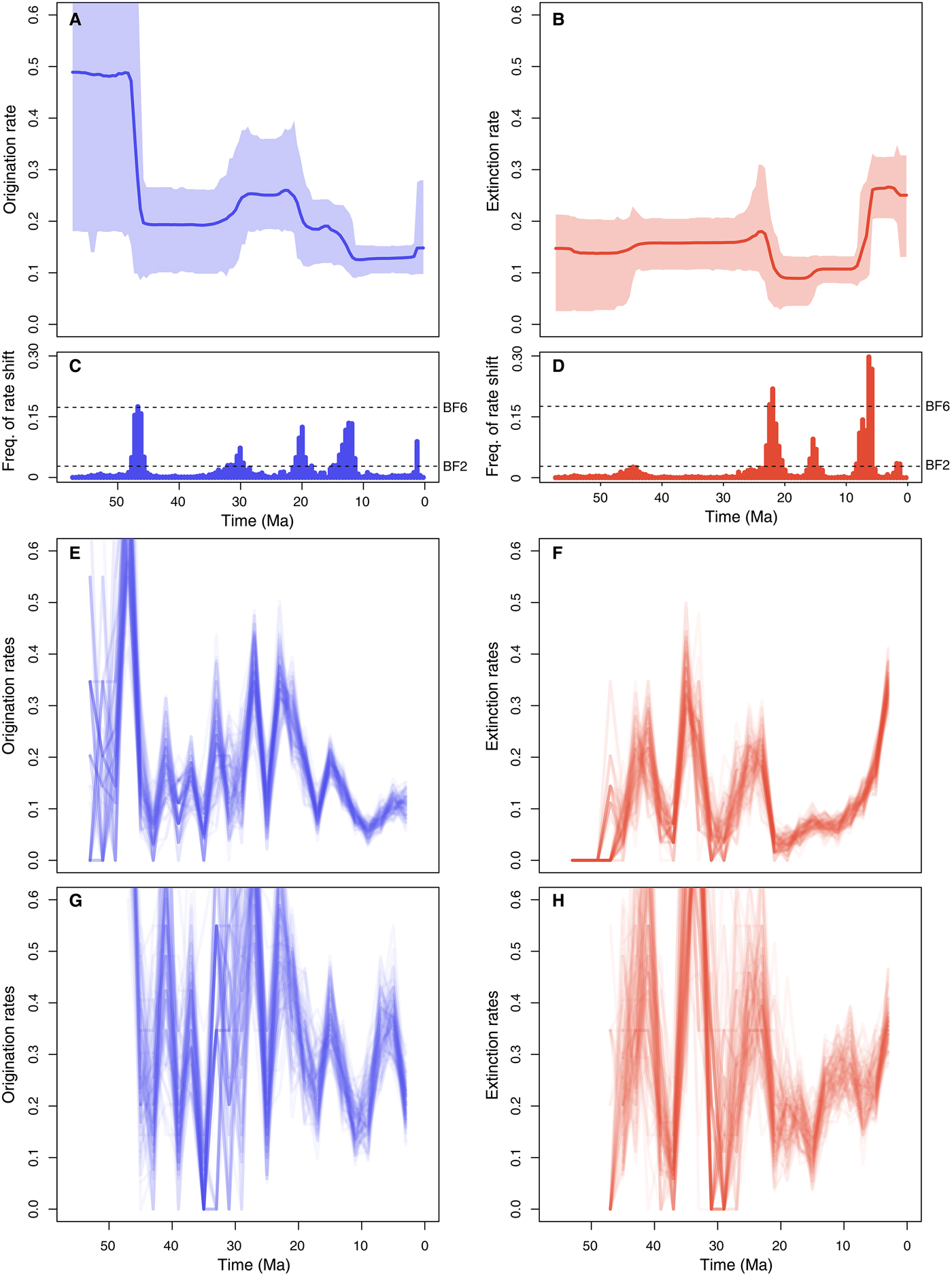
Figure 5. Origination and extinction rates through time in marine mammals. Marginal posterior estimates of origination rates (A) and extinction rates (B) are shown together with the respective 95% credible intervals. These estimates incorporate not only parameter uncertainty, but also dating uncertainties (deriving from 10 replicated analyses obtained by resampling the ages of the fossil occurrences) and uncertainties around model selection, as the reversible jump Markov Chain Monte Carlo algorithm samples the number of rate shifts from their joint posterior distribution. Plots on the right show the frequency of sampling a shift in origination (C) and extinction (D) rates within arbitrarily small time bins (here set to 0.5 Myr). Dashed lines show log Bayes factors of 2 and 6 (as inferred from Markov chain Monte Carlo simulation). Sampling frequencies exceeding these lines indicate positive and strong statistical evidence for a rate shift, respectively. For comparison, origination and extinction rate estimates were also inferred under the boundary-crossing method (E, F) (Foote Reference Foote2000) and the three-timer approach (G, H) (Alroy Reference Alroy2014). The ages of fossil occurrences were randomized 100 times based on the respective stratigraphic intervals (as in the PyRate analyses), and the rates were estimated using equal time bins of 2 Myr.
Inferred extinction rates (Fig. 5B) were stable across most of the Eocene and Oligocene and dropped in the early Miocene. The rates then increased dramatically during the late Miocene and high levels of extinctions were inferred for the Pliocene and Pleistocene, although we estimated a mild rate decrease in the middle Pleistocene. Bayes factors indicated strong support (i.e., 2log BF>6) for rate shifts 23–21 and 6.25–5.75 Ma and positive support of shifts 16–15 and 1.25–1.75 Ma (Fig. 5D).
The origination and extinction rates obtained from the boundary-crossing and three-timer methods broadly follow the trajectories estimated using PyRate but display a substantially higher number of fluctuations, particularly in the Paleogene, where rates appear to vary by up to one order of magnitude across adjacent time bins (Fig. 5E–H). Both methods indicate an increase in extinction rates toward the recent, although it is difficult to pinpoint when the extinction rates began to increase.
Performance of the FastPyRatec Library
The new C++ library dramatically boosted the PyRate performance, with different levels of speed-up depending on the underlying model and the size of the data set. In our tests, the C++ version was between five and eight times faster than the Python implementation when using the HPP model of preservation. Under the TPP model, the speed-up reached 26 times for a data set of 300 taxa (Supplementary Fig. S9). This performance improvement has a very significant impact on the feasibility of analyzing large data sets. For instance, an analysis of 300 taxa with the TPP model, running 10 million RJMCMC iterations (default in PyRate) on a reasonably fast CPU, takes about 3 hours using the FastPyRateC library, whereas it takes around 3 days using the all-Python version. The magnitude of this performance boost becomes crucial when it comes to the analysis of large empirical data sets. The analysis of Cenozoic marine mammals presented in this study (more than 500 taxa, 50 million MCMC iterations) takes about 14 h on a 3.1 GHz CPU, using the C++ library. In contrast, the same analysis performed using the Python implementation would need more than 19 days to complete (i.e., more than 30 times longer).
Discussion
Inferring Macroevolutionary Rates from Fossils
A large proportion of macroevolutionary research processes with the aim of understanding how biodiversity has evolved through time and space and what drives the rise and demise of clades in the tree of life (e.g., Raup and Sepkoski Reference Raup and Sepkoski1984; Raup Reference Raup1986; Foote et al. Reference Foote, Crampton, Beu, Marshall, Cooper, Maxwell and Matcham2007; Alroy Reference Alroy2008; Quental and Marshall Reference Quental and Marshall2013; Benton et al. Reference Benton, Forth and Langer2014; Cantalapiedra et al. Reference Cantalapiedra, Fernández, Azanza and Morales2015; Ezard et al. Reference Ezard, Quental and Benton2016). The fossil record has been used to infer diversification and extinction processes for a long time and arguably provides for many lineages (e.g., any organism with a mineralized skeleton), the most informative available data for understanding macroevolutionary dynamics (Marshall Reference Marshall2017).
PyRate is a software designed to analyze fossil data in a Bayesian framework. Its main strengths are: (1) enabling users to analyze the entire fossil occurrence record (i.e., not only first and last appearances) and all described lineages (including singletons and extant taxa), (2) incorporating parameter uncertainties using Bayesian algorithms, and (3) using explicit probabilistic model selection to adequately infer the complexity of the preservation and birth–death models based on the data. Because fossil data are often limited in size, it is essential to adequately quantify the uncertainty around each parameter estimate to avoid interpreting the results with a false sense of precision. Thus, the use of a Bayesian framework is well suited for the task, providing credible intervals for each parameter rather than point estimates and simultaneously integrating the uncertainties associated with all parameters (Gelman et al. Reference Gelman, Carlin, Stern and Rubin2013).
Methodological Advances
We presented a flexible and powerful suite of quantitative methods to infer macroevolutionary processes using fossil occurrence data. Preservation processes are typically modeled by constant or time-varying sampling probabilities (Foote Reference Foote2000; Liow and Nichols Reference Liow, Nichols, Hunt and Alroy2010; Bapst and Hopkins Reference Bapst and Hopkins2016), which are, however, assumed to be constant across lineages. Here, we developed a new model in which a preservation process with time-variable mean rates can be coupled with rate heterogeneity across lineages. Both types of rate variations are expected to be ubiquitous, reflecting temporal environmental changes, which may affect sedimentation and fossilization processes as well as preservation biases associated with each organism (lifestyle, anatomy, size, and other traits, e.g., shell composition [Foote et al. Reference Foote, Crampton, Beu and Nelson2015]). We also presented a novel likelihood-based test allowing a formal statistical comparison among alternative preservation models. This procedure facilitates an objective, data-driven selection of the most appropriate model of fossil preservation. As expected, our model incorporating rate heterogeneity both through time and among lineages is indeed supported by empirical data against the alternative models, as shown with the marine mammals analyzed here. We note that the parameterization of the preservation process and the priors used here are designed for general-purpose analyses and do not include additional empirical evidence beyond the temporal distribution of fossil occurrences for each species. Thus, while the rate heterogeneity across lineages inferred from empirical data sets may reflect preservation potentials due to different anatomical and life-history traits, this information is not provided a priori in the analysis. Similarly, the preservation process is affected by the amount of available rock volume and is likely characterized by strong geographic biases that are not explicitly accounted for by our model. Future developments should incorporate additional information about these sampling biases, potentially building upon previously demonstrated analytical methods (Sadler et al. Reference Sadler, Kemple and Kooser2008; Wagner and Marcot Reference Wagner and Marcot2013; Foote et al. Reference Foote, Crampton, Beu and Nelson2015; Silvestro et al. Reference Silvestro, Zizka, Bacon, Cascales-Miñana, Salamin and Antonelli2016).
We implemented a new algorithm that uses RJMCMC to estimate birth–death processes and jointly infer (in addition to the preservation parameters) the number and temporal placement of rate shifts and marginal origination and extinction rates through time. We found RJMCMC to outperform the previously implemented BDMCMC algorithm, providing more accurate rates and estimated numbers of shifts. The main advantages of RJMCMC are that (1) it provides marginal rates that account for uncertainties in the time and number of rate shifts, (2) it allows us to easily compute Bayes factors to assess statistically significant times of rate shift, and (3) its prior on the number of rate shifts is itself estimated from the data (unlike in BDMCMC, where it is fixed a priori [Silvestro et al. Reference Silvestro, Schnitzler, Li, Antonelli and Salamin2014b]), thus making the algorithm more versatile and able to adapt to different data sets.
Whereas several methods have been developed to infer rate variation in origination and extinction rates through time (e.g., Foote Reference Foote2001, Reference Foote2003; Liow and Nichols Reference Liow, Nichols, Hunt and Alroy2010; Alroy Reference Alroy2014, Reference Alroy2015; Liow and Finarelli Reference Liow and Finarelli2014; Foote et al. Reference Foote, Crampton, Beu and Nelson2015), these approaches do not explicitly assess the minimum number of parameters required to accurately describe the data, that is, the best-fitting model. The suite of methods presented here implements probabilistic tests and algorithms that specifically tackle this issue. The number of parameters included in preservation models and birth–death models in PyRate is determined by the information intrinsic to the data, rather than a priori. The result of this approach is a direct estimation of when and how many times the pace of diversification has changed throughout the history of a clade. With the implementation of the new RJMCMC algorithm, the timing of rate changes is itself estimated through Bayes factors to assess its significance (Fig. 5B,C). A similar approach had been used before in a phylogenetic (neontological) context (May et al. Reference May, Höhna and Moore2016) but, to the best of our knowledge, was not available in the analysis of paleontological data.
The approach presented here models preservation, origination, and extinction as continuous-time processes. Most other methods (e.g., boundary-crossing and three-timer) are based on discrete time, whereby the ages of the fossil occurrences are translated into presence or absence within a predefined time bin. Although the true nature of natural processes such as species appearance and disappearance is obviously time continuous, the choice of binned data reflects the fact that most occurrences are not dated directly, but instead assigned to temporal ranges based on their respective stratigraphic units (Foote and Miller Reference Foote and Miller2007). In PyRate we treat these temporal ranges as uncertainties in the dating and resample them randomly to incorporate such uncertainties in the analyses (see also Analysis Protocol for Marine Mammals, Supplementary Material). In a discrete-time analysis assuming two bins for the Pliocene or the Pleistocene, one could assign fossil occurrences to either of the two epochs. However, under these settings, even an occurrence dated with higher precision (e.g., assigned to the Piacenzian) will be treated as “Pliocene,” therefore ignoring the additional information. In contrast, one advantage of our approach is that each occurrence (or all occurrences from each fossil assemblage) will be assigned its own uncertainty range.
The parameterization of the PyRate model and the algorithms implemented to carry out parameter estimation and model testing necessarily result in a more computationally demanding approach compared with alternative methods. To alleviate this potential bottleneck, we implemented a new C++ library, which yields considerable speed-up compared with previous versions of the software (orders of magnitude; Supplementary Fig. S9). This and the ever-increasing performance of computers and clusters make PyRate a suitable method even for relatively large data sets.
Importance of Model Testing in Estimating Origination and Extinction: Comparing PyRate with Other Methods
Using a robust and explicit model selection framework is crucial to avoid overparameterization, and this represents one of the biggest novelties of the methods presented here, compared with other approaches. Indeed, assuming origination and extinction rates to be independent parameters in predefined time bins (i.e., without explicitly model testing) is common practice in paleobiological studies of macroevolution (Foote Reference Foote2003; Liow and Finarelli Reference Liow and Finarelli2014; Alroy Reference Alroy2015; but see Connolly and Miller Reference Connolly and Miller2001; Foote Reference Foote2007). However, this practice may generate spurious results if the amount of data is insufficient to confidently estimate all the parameters (Smiley Reference Smiley2018), which is a general problem with overparameterization and overfitting (Burnham and Anderson Reference Burnham and Anderson2002). The RJMCMC algorithm presented here and the other algorithms implemented in PyRate infer the amount of rate variation directly from the data. Although we focused here on algorithms that simultaneously optimize the parameters and the model (RJMCMC and BDMCMC), other methods to avoid overparameterization are available in PyRate, based on the estimation of model marginal likelihoods (Silvestro et al. Reference Silvestro, Schnitzler, Li, Antonelli and Salamin2014b), Bayesian variable selection (Silvestro et al. Reference Silvestro, Antonelli, Salamin and Quental2015a), and Bayesian shrinkage (Silvestro et al. Reference Silvestro, Cascales-Miñana, Bacon and Antonelli2015b, Reference Silvestro, Pires, Quental and Salamin2017). Using these methods, the complexity of the model adapts to the signal provided by the data and its statistical power, so that only statistically significant rate changes are identified. This procedure also provides a formal approach to assess whether apparent rate variations are not just the result of the stochastic nature of a constant-rate birth–death process.
The levels of accuracy obtained by our RJMCMC algorithm were up to 10 times higher than with other methods when the true underlying model was a time-homogeneous birth–death process (Supplementary Fig. S6). This is clearly a case in which assuming independent rates per time bin represents an overparameterization of the true process. Indeed, the difference in accuracy between rate estimates from the boundary-crossing and three-timer methods and rates inferred in PyRate tended to decrease when the true underlying model included rate shifts. We interpret this as a consequence of the fact that the true speciation and extinction dynamics in these simulations better conform to models with independent rates per time bin. Yet even under simulations characterized by a high rate heterogeneity through time (scenario 3), PyRate accuracy was substantially higher than with the other methods (Supplementary Fig. S8).
While a comprehensive comparison between all available methods to infer origination and extinction rates from fossil data is beyond the scope of this study (but see Smiley [Reference Smiley2018] for a recent and extensive simulation study), our results clearly indicate that there are substantial benefits associated with the use of explicit model testing to prevent overparameterization. The optimization of the complexity of the model based on the data is crucial to obtaining realistic estimates of diversification processes from incomplete fossil data. Based on these results, we recommend always verifying the statistical support for the number of model parameters when inferring diversification dynamics from fossil data.
Conclusions
PyRate is an open-source project to which researchers are welcome to contribute code, ideas, and feedback through its online repository. It includes many birth–death models for taxonomic diversification as well as several preservation models in which rates can vary through time and across lineages. The hierarchical Bayesian methods implemented in PyRate allow users to assess the statistical support of different models and to jointly infer all the parameters. We have shown that explicit model testing when inferring origination and extinction rates yields substantially improved accuracy. As a by-product of the Bayesian algorithms used in PyRate, credible intervals are inferred for all model parameters (e.g., preservation, origination, and extinction rates) and can be used to quantify the level of uncertainties surrounding the estimates.
Although we focused here on diversification processes in which origination and extinction rates change through time, several other models have been implemented in PyRate enabling users to test specific hypotheses about, for example, diversity-dependent diversification with competition within and among clades (Pires et al. Reference Pires, Silvestro and Quental2017), correlations to biotic and abiotic factors (Lehtonen et al. Reference Lehtonen, Silvestro, Karger, Scotese, Tuomisto, Kessler, Peña, Wahlberg and Antonelli2017), and age-dependent and trait-dependent extinction rates (Hagen et al. Reference Hagen, Andermann, Quental, Antonelli and Silvestro2017; Piras et al. Reference Piras, Silvestro, Carotenuto, Castiglione, Kotsakis, Maiorino, Melchionna, Mondanaro, Sansalone, Serio, Vero and Raia2018). The versatility of a fully probabilistic Bayesian method to infer diversification dynamics allows for the development of additional models and algorithms to tackle specific questions. For example, a model of pulsed turnover (Vrba Reference Vrba1985) might be better captured by an algorithm that, rather than looking for rate shifts, clusters time bins by the magnitude of the origination and extinction rates, one example being the Dirichlet process prior method (Neal Reference Neal2000) (a prototype of which is already available in the current version of PyRate). In conclusion, PyRate provides a flexible, statistically sound analytical framework enabling researchers to analyze the growing amount of available fossil occurrence data, and we think it can serve as a useful tool kit for many future studies in paleobiology.
Software Availability
All the models described in this study are implemented within the open-source package PyRate and are available at: https://github.com/dsilvestro/PyRate. The program is written in Python 2.7 and R and has been tested under the major operating systems (MacOS, Windows, and several Linux distributions). A detailed command list and tutorials are available in the GitHub repository.
Importantly, PyRate requires a minimum number of a priori decisions from the user, and while each setting can be accessed through specific commands, default values and settings are set to adapt to most data sets. PyRate runs as a stand-alone command-line program, and running the software does not require any knowledge of Python from the user. The program also includes many utility functions that can be used to plot and summarize the results, process multiple output files, and parse large data sets to identify potential spelling variation in taxon names using a built-in machine-learning classifier (as shown in the Supplementary Material).
To provide easy access to the augmented performance of the FastPyRateC library, precompiled modules for 64-bit versions of Windows, MacOS, and Linux are available on the PyRate Github repository, in addition to the source code.
Acknowledgments
All analyses were run at the High-Performance Computing Center (Vital-IT) at the Swiss Institute of Bioinformatics. D.S. received funding from the Swedish Research Council (2015-04748). N.S. received funding from the University of Lausanne (Switzerland) and the Swiss National Science Foundation (CR32I3-143768). A.A. received funding from the Swedish Foundation for Strategic Research, the Swedish Research Council (B0569601), the Faculty of Sciences at the University of Gothenburg, and a Wallenberg Academy Fellowship. X.M. received funding from the Swiss National Science Foundation (P2GEP2_178032). We are thankful to M. Patzkowsky, P. Wagner, A. Dunhill, R. Warnock, and one anonymous reviewer for valuable feedback on this work. We thank T. Smiley, B. McHorse, M. Crotti, T. Hauffe, J. L. Cantalapiedra, O. Inostroza, T. B. Quental, M. M. Pires, and E. Gjesfjeld for discussion and feedback on the software. We thank E. Orliac of the Scientific Computing and Research Support Unit, University of Lausanne (Switzerland) for support on the Windows version of FastPyRateC.


 Open access