


1. Introduction
The atmosphere has an abrupt transition in buoyancy frequency  $N$ at the tropopause (Birner, Dornbrack & Schmann Reference Birner, Dornbrack and Schmann2002), increasing with altitude by a factor of 2 approximately. This feature causes reflection of upward-propagating internal waves, as well as a localized mean flow. The behaviour of internal waves at the tropopause is important to weather and climate, and may result in dynamical features that are hazardous to commercial aircraft at cruising altitudes.
The transition region is thin (Birner et al. Reference Birner, Dornbrack and Schmann2002), much less than a typical vertical wavelength of internal waves in Earth's atmosphere (2–10 km). The sharpness of this transition suggests a two-layer approximation, where the transition region is replaced with a sharp interface in  $N$ with continuous density. This interfacial model of the tropopause has a long history (Scorer Reference Scorer1949) and is sometimes referred to as a density-gradient interface.
McHugh (Reference McHugh2009) and Mathur & Peacock (Reference Mathur and Peacock2009) considered internal waves impinging from below on a density-gradient interface. Mathur & Peacock (Reference Mathur and Peacock2009) treated linear wave beams with single and multiple interfaces. McHugh (Reference McHugh2009) considered weakly nonlinear uniform waves with a single interface. The results of McHugh (Reference McHugh2009) show that a primary harmonic (wave of frequency  $\sigma$) has higher harmonics (components with frequency $2 \sigma$, $3 \sigma$, etc.) that accumulate at the interface, much like free surface waves. This feature does not happen away from the interface for a monochromatic wavetrain, since the linear solution is also an exact nonlinear solution as long as $N$ is constant, the waves are uniform, and the flow is Boussinesq. Thus the region in the vicinity of the sharp interface will have stronger nonlinear effects than other altitudes. Both McHugh (Reference McHugh2009) and Mathur & Peacock (Reference Mathur and Peacock2009) report that linear reflection and transmission coefficients obey Snell's law from the theory of optics.
Grimshaw & McHugh (Reference Grimshaw and McHugh2013) and McHugh (Reference McHugh2015) considered amplitude equations for a packet of ascending internal waves incident upon a density-gradient interface. The buoyancy frequency was constant in each layer, with a sudden change in value at the interface. The waves were horizontally periodic but slowly varying in the vertical, resulting in nonlinear Schrödinger (NLS) equations for incident, reflected and transmitted wave packets. The results show that the wave-induced mean flow is discontinuous at the interface, assuming inviscid flow. Furthermore, the incident and reflected waves combine for a short period to create a strong localized mean flow under the interface. The NLS equations in McHugh (Reference McHugh2015) neglected the effect of the mean buoyancy. Mean buoyancy has been included here, with results showing only minor differences.
Grimshaw & McHugh (Reference Grimshaw and McHugh2013) derive the weakly nonlinear interfacial conditions for a general interface, but then neglect the nonlinear interfacial effects. The result is reflection and transmission coefficients that are accurate to  $O(\alpha )$, where $\alpha$ is the amplitude parameter. In contrast, the NLS amplitude equations that are valid in the fluid interior are accurate to third order (Grimshaw Reference Grimshaw1975; Shrira Reference Shrira1981; Voronovich Reference Voronovich1982). The interfacial conditions are extended here to include effects up to third order, matching the accuracy of the amplitude equations, and making the interfacial conditions nonlinear.
A related configuration but with constant  $N$ throughout (no interface) has been treated previously by many authors (Grimshaw Reference Grimshaw1975; Shrira Reference Shrira1981; Voronovich Reference Voronovich1982; Sutherland Reference Sutherland2001, Reference Sutherland2006; Tabaei & Akylas Reference Tabaei and Akylas2007). Often, a Gaussian wave packet is created at the bottom boundary (Sutherland Reference Sutherland2001, Reference Sutherland2006; Tabaei & Akylas Reference Tabaei and Akylas2007), which then evolves as the wave packet ascends. If the waves propagate at a steep angle such that $n < k$, where $n$ and $k$ are the vertical and horizontal wavenumbers, respectively, then the wave packet will focus energy as a result of the combination of nonlinear and dispersive effects (Sutherland Reference Sutherland2001). Waves propagating at a shallow angle will defocus energy (Sutherland Reference Sutherland2001). The evolution depends on parameter values, and also on the distance from the wavemaker. The results given below neglect this evolution of the incident wave packet, and prescribe the incident waves at the interface as the Gaussian profile, and sometimes the ‘raised cosine’ profile. Prescribing the incident wave amplitude allows easier interpretation of the reflected and incident wave amplitudes.
Density profiles with a density interface (jump in density  $\Delta \rho$) have also been used to study internal wave reflection. Delisi & Orlanski (Reference Delisi and Orlanski1975) performed experiments with a two-layer configuration, where the upper layer had linearly increasing density with depth, and the lower layer had constant density, with a jump in density at the interface of the two layers. Internal wave beams were created in the upper layer that impinged on the interface and were reflected. They use a linear theory for uniform internal waves to predict that the reflected wave amplitude is equal to the incident wave amplitude at the interface, as expected since internal waves cannot propagate into the bottom layer with its constant density. The linear theory also predicts the phase shift and the amplitude of the interface, showing good agreement with their experimental results for a sequence of values of $\Delta \rho$.
Thorpe (Reference Thorpe1998) treated wave reflection also using a two-layer density profile with a density jump at the interface. The upper layer was constant density and finite thickness, while the lower layer had density increasing with depth, a simplified model of the oceanic density profile. Thorpe predicts that the amplitude of the primary component of the reflected waves is equal to the amplitude of the incident waves, as in Delisi & Orlanski (Reference Delisi and Orlanski1975). Thorpe then determines the amplitude and phase of the second-order component of the reflected wave for the case where the incident waves are uniform. This second-order amplitude is dependent on the density jump at the interface and the thickness of the upper layer, as well as the incident wave parameters.
Diamessis et al. (Reference Diamessis, Wunsch, Delwiche and Richter2014) treat reflection of internal wave beams using numerical simulations. They also employ a density profile that models the ocean, with a constant-density upper layer, a stratified lower layer with constant  $N$, and a finite-thickness transition region that has peak value of $N$ (a pycnocline). The results show wave activity within the transition layer that extends downstream of the incident wave impact region, ultimately re-radiating internal waves. Experiments by Wunsch et al. (Reference Wunsch, Delwiche, Frederick and Brandt2015) confirm the presence of these oscillations in the transition region. Thus the concept of wave reflection is too simple for some circumstances, such as when the transition between layers is thick.
Energy dissipation of internal waves by the creation of higher harmonics when  $N$ is non-uniform has been treated recently by Sutherland (Reference Sutherland2016), Wunsch (Reference Wunsch2017, Reference Wunsch2018), Varma & Mathur (Reference Varma and Mathur2017) and Baker & Sutherland (Reference Baker and Sutherland2020). In all of these studies the profile of $N$ was chosen to model an oceanic pycnocline, with its rapidly changing $N$. Sutherland (Reference Sutherland2016) treated a smooth $N$ profile, and initiated nonlinear simulations with a low-order eigenmode. They found that higher harmonics formed where $N$ was changing most rapidly. Wunsch (Reference Wunsch2017) used a piecewise-constant $N$ profile and weakly nonlinear theory to determine the second harmonic at second order in wave amplitude. Wunsch (Reference Wunsch2018) then extended the theory to a more complex $N$ profile. Varma & Mathur (Reference Varma and Mathur2017) treated a smooth $N$ profile and included a pair of primary modes. Weakly nonlinear theory again shows that higher harmonics are generated where $N$ is rapidly changing, and that a wave beam incident upon the pycnocline generates a reflected second harmonic at second order. Baker & Sutherland (Reference Baker and Sutherland2020) include a primary (parent) mode and a second harmonic in a smooth exponential $N$ profile. The amplitude of the second harmonic is time-dependent, and the results show ‘beat’ phenomena. The results given here treat the nonlinear aspects of the primary harmonic, which appear at third order in wave amplitude.
The nonlinear interfacial conditions developed here are accurate to third order, matching the accuracy of the amplitude equations. These nonlinear interfacial effects create a second harmonic at second order, and a correction to the reflection and transmission amplitudes of the primary harmonic at third order. This third-order correction is the main issue treated here. The final interfacial conditions contain products of incident, reflected and transmitted wave amplitudes, thus are nonlinear and are treated numerically.
Higher-order linear terms appear formally in the interfacial conditions. The higher-order linear terms result in a homogeneous part to the reflected and transmitted wave amplitudes. For steep waves, the homogeneous solution indicates exponential growth, indicating that the wave solution is unstable at the interface. Numerical evaluation of the nonlinear interfacial conditions agrees with the linear result, also showing exponential growth for steep waves. This instability may explain the previous observations over Hawaii by McHugh et al. (Reference McHugh, Dors, Jumper, Roadcap, Murphy and Hahn2008), showing large values of vertical velocity only at the tropopause altitude.
For less steep waves, linear theory shows that the homogeneous part is exactly zero for any packet length. But when the packet length is relatively short, the numerical linear results have erroneous homogeneous oscillations. The asymptotic theory assumes a long packet, thus these erroneous cases are outside the validity of the theory. However, nonlinear effects for shorter packets are investigated here by neglecting the higher-order linear terms while retaining the nonlinear terms.
Overall, the results show that nonlinear wave reflection of the primary harmonic is less than the linear reflection for all parameter values. Similarly, the nonlinear wave transmission is always greater than the linear transmission. Thus nonlinear effects cause the interface to be more transparent to internal waves.
Section 2 quotes the basic equations and develops the weakly nonlinear interfacial conditions. Section 3 introduces the packet of carrier waves, but only sketches the derivation of the amplitude equations governing the packet away from the interface, since this has been published previously (Sutherland Reference Sutherland2006; Grimshaw & McHugh Reference Grimshaw and McHugh2013; McHugh Reference McHugh2015). However the interfacial conditions in terms of wave amplitudes are developed thoroughly in § 3, as the nonlinear part has not been treated previously. Unfortunately the derivation of the nonlinear interfacial conditions is complex, making § 3 somewhat tedious. Section 4 discusses linear results, including the effect of the higher-order linear terms. Section 5 discusses the nonlinear results. Finally § 6 summarizes and provides conclusions.
2. Basic equations
The flow is treated as incompressible, inviscid and two-dimensional, and the background rotation is neglected. The flow is then governed by
 \begin{gather} \left( \rho_0 + \rho \right) \frac{{\rm D} u}{{\rm D} t} ={-} \frac{\partial p}{\partial x}, \end{gather}
 \begin{gather}\left( \rho_0 + \rho \right) \frac{{\rm D} w}{{\rm D} t} ={-} \frac{\partial p}{\partial z} - \rho g, \end{gather}
 \begin{gather}{\frac{\partial u}{\partial x}} + {\frac{\partial w}{\partial z}} = 0, \end{gather}
 \begin{gather}{\frac{{\rm D} \rho}{{\rm D} t}} - {N^2}\,\frac{\rho_0}{g}\,w = 0, \end{gather}
where
 \begin{equation} {\frac{{\rm D}}{{\rm D} t}} = {\frac{\partial}{\partial t}} + u\,{\frac{\partial}{\partial x}} + w\, {\frac{\partial}{\partial z}}, \end{equation}
the velocity is  $(u, w)$, the dynamic pressure is $p$,
$p$,  $\rho _0 (z)$ is the base-state density, $\rho$ is the disturbance density, and $N$ is defined by
 \begin{equation} N^2 ={-} \frac{g {\rho_0}_z}{\rho_0}. \end{equation}
It will be useful to employ the field  $\zeta (x,z,t)$, which is vertical displacement of material lines. The kinematic relationship between velocity and $\zeta$ is
 \begin{equation} \frac{{\rm D} \zeta}{{\rm D} t} = w. \end{equation}
The interfacial conditions between any two layers in a stratified fluid are developed in Grimshaw & McHugh (Reference Grimshaw and McHugh2013). In general, the interface may have a jump in density or buoyancy frequency. The kinematic condition on the interface is continuity of normal velocity. This condition is treated in the usual manner, with
 \begin{equation} \eta_t + u \eta_x = w \end{equation}
on  $z = \eta$, using velocity components for each layer. Since the interface is also a material line, the kinematic interfacial condition is merely
 \begin{equation} \zeta = \eta \end{equation}
on  $z = \eta$. Using a Taylor series in the usual way, (2.9) becomes
 \begin{equation} \zeta + \zeta_z \eta + \tfrac{1}{2} \zeta_{zz} \eta^2 + \cdots = \eta \end{equation}
on  $z=0$. This expression may be used recursively (Grimshaw & McHugh Reference Grimshaw and McHugh2013) to get
 \begin{equation} \eta = \zeta + \zeta \zeta_z + \zeta \zeta_z^2+ \tfrac{1}{2} \zeta^2 \zeta_{zz} + \cdots \end{equation}
on  $z=0$. The kinematic condition may now be written as
 \begin{equation} [\zeta + \zeta \zeta_z + \zeta \zeta_z^2 + \tfrac{1}{2} \zeta^2 \zeta_{zz} + \cdots]_-^+ = 0 \end{equation}
on  $z = 0$.
The dynamic condition at the interface is continuity of total pressure:
 \begin{equation} [ p_0 + p ]_-^+ = 0 \end{equation}
on  $z = \eta$, where $p_0 (z)$ is the base-state hydrostatic pressure. Using a Taylor series in (2.13) produces
 \begin{equation} [( p + p_0) + ( p_z + {p_0}_z ) \eta + \tfrac{1}{2}
( p_{zz} + {p_0}_{zz} ) \eta^2 + \tfrac{1}{6}
( p_{zzz} + {p_0}_{zzz} ) + \cdots]_-^+ =
0 \end{equation}
\begin{equation} [( p + p_0) + ( p_z + {p_0}_z ) \eta + \tfrac{1}{2}
( p_{zz} + {p_0}_{zz} ) \eta^2 + \tfrac{1}{6}
( p_{zzz} + {p_0}_{zzz} ) + \cdots]_-^+ =
0 \end{equation}
on  $z = 0$. The base-state pressure is continuous at all positions, thus
 \begin{equation} p_0|_-^+ = 0. \end{equation}
Equation (2.14) is used recursively to evaluate derivatives of disturbance pressure. Furthermore, the variable  $\eta$ is eliminated from the dynamic condition using (2.11). After some manipulation, the dynamic interfacial condition becomes
 \begin{equation} \left[p - \rho_0 g \zeta - \frac{1}{2}\,\rho_0 N^2 \zeta^2 + \frac{1}{6}\,\rho_0 \left(\frac{{\rm d}N^2}{{\rm d}z} - \frac{N^4}{g} \right) \zeta^3\right]_-^+ = 0, \end{equation}
on  $z = 0$, where higher-order terms have been dropped. Equation (2.16) is valid for any interface, including discontinuous $\rho _0$ and/or $N$.
$N$.
With continuous density  $\rho _0$ and discontinuous $N$, but $N$ constant in each layer, (2.16) reduces to
 \begin{equation} \left[p - \frac{1}{2}\,\rho_0 N^2 \zeta^2- \frac{1}{6}\,\rho_0\,\frac{N^4}{g}\,\zeta^3\right]_-^+ = 0 \end{equation}
on  $z=0$.
3. The amplitude equations
3.1. Away from the interface
A packet of monochromatic waves is assumed to impinge on the interface from below. The wave amplitude  $\alpha$ is assumed small, and all dependent variables are expanded in a power series in $\alpha$:
 \begin{equation} \zeta = \alpha \zeta^{(1)} + \alpha^2 \zeta^{(2)} + \alpha^2 \bar{\zeta} + \cdots, \end{equation}
and similarly for  $u,w,\rho,p$, where the superscript indicates the order of the approximation. Here, $\bar {\zeta }$ is the wave-induced mean. Previous theory (Shrira Reference Shrira1981) has shown that the wave-induced mean is non-zero at second order. This mean part is separated from the oscillatory second-order solution merely for convenience.
An upwardly propagating internal wave has the leading-order solution
 \begin{equation} \zeta^{(1)} = I E \exp({-{\rm i} n_1 z}) + I^* E^* \exp({{\rm i} n_1 z}), \end{equation}
with
 \begin{equation} E = \exp({{\rm i}(kx - \sigma t)}), \end{equation}
where  $I$ is the incident wave amplitude, $k$ is the horizontal wavenumber, $n_1$ is the vertical wavenumber, and $\sigma$ is the wave frequency, all assumed positive and real. However, this solution alone cannot meet the interfacial conditions, which require a reflected and transmitted wave at this order. Following Grimshaw & McHugh (Reference Grimshaw and McHugh2013) and McHugh (Reference McHugh2015), the leading-order solution including reflected and transmitted waves is
 \begin{gather} \zeta^{(1)} = I E \exp({-{\rm i} n_1 z}) + I^* E^* \exp({{\rm i} n_1 z}) + R E \exp({{\rm i}n_1 z}) + R^* E^* \exp({-{\rm i} n_1 z}),\quad z<0, \end{gather}
 \begin{gather}\zeta^{(1)} = T E \exp({-{\rm i} n_2 z}) + T^* E^* \exp({{\rm i} n_2 z}),\quad z>0, \end{gather}
where  $n_1,n_2$ are the vertical wavenumbers in the lower and upper layers, respectively, and $R,T$ are the reflected and transmitted wave amplitudes, respectively. All terms proportional to $E$ will be called the primary harmonic, while the secondary harmonic has $E^2$, and so on. Thus the above expression for $\zeta ^{(1)}$ contains only the primary harmonic. The secondary harmonic will appear in $\zeta ^{(2)}$ as a result of nonlinear effects in the interfacial conditions.
The wave amplitude is chosen to be vertically modulated but horizontally uniform, as in Sutherland (Reference Sutherland2006), Grimshaw & McHugh (Reference Grimshaw and McHugh2013) and McHugh (Reference McHugh2015). The parameter  $\epsilon$ is defined to be the inverse of the packet length, normalized by the horizontal wavenumber $k$. This makes $\epsilon$ proportional to the ratio of horizontal wavelength to vertical packet length. A solution is obtained by assuming that the packet is long, making $\epsilon$ small. Slow variables are introduced to achieve this solution:
 \begin{equation} \left.\begin{gathered} t_j = \epsilon^j t,\\ z_j = \epsilon^j z, \end{gathered}\right\} \end{equation}
with  $j = 1,2$. The amplitude functions $I,R,T$ all depend on these slow variables,
The waves create a wave-induced mean flow, as discussed in Grimshaw & McHugh (Reference Grimshaw and McHugh2013). The mean is defined here as a horizontal average ( $x$-average), denoted with an overbar. The components of the mean solution that are needed for the interfacial conditions are $\bar {\zeta }$ and $\bar {u}$, which may be determined to second order using
 \begin{equation} \left.\begin{gathered} \alpha^2 \bar{\zeta} ={-} \frac{1}{2}\,\frac{\partial}{\partial z}\langle \zeta^2 \rangle,\\ \alpha^2 \bar{u} = \frac{k}{\sigma}\,N^2 \langle \zeta^2\rangle, \end{gathered}\right\} \end{equation}
where the angle brackets mean average. Using (3.4) and (3.5) in these equations gives (Grimshaw & McHugh Reference Grimshaw and McHugh2013)
 \begin{gather} \bar{\zeta} ={-} {\rm i} 2 n_1 ( I^* R \exp({{\rm i} 2 n_1 z}) - I R^* \exp({-{\rm i} 2 n_1 z})),\quad z < 0, \end{gather}
 \begin{gather}\bar{u} = 2 N_1^2\,\frac{k}{\sigma} [I I^* + R R^* + I^* R \exp({{\rm i} 2 n_1 z}) + I R^* \exp({-{\rm i} 2 n_1 z})],\quad z < 0, \end{gather}
 \begin{gather}\bar{u} = 2 N_2^2\,\frac{k}{\sigma}\,T T^*,\quad z > 0, \end{gather}
and  $\bar {\zeta } = 0$ for $z>0$.
The governing equations (2.1)–(2.7) may be written as
 \begin{gather} \rho_0 \left( u_t + Q_1 \right) ={-} \frac{\partial p}{\partial x}, \end{gather}
 \begin{gather}\rho_0 \left( w_t + Q_3 \right) ={-} \frac{\partial p}{\partial z} - \rho g, \end{gather}
 \begin{gather}u_x + w_z = 0, \end{gather}
 \begin{gather}\rho_t + Q_4 - {N^2}\,\frac{\rho_0}{g}\,w = 0, \end{gather}
 \begin{gather}\zeta_t + Q_5 = w, \end{gather}
where the  $Q_j$ are the sums of the nonlinear terms in each equation. Eliminate all variables in the linear terms except $\zeta$ to achieve
 \begin{align} &\frac{\partial^3}{\partial t^3}\left( \zeta_{xx} + ( \rho_0 \zeta_z )_z \right)+ \rho_0 N^2 \zeta_{xxt} \nonumber\\ &\quad = (\rho_0 {Q_1}_{xt} )_z- \rho_0 {Q_3}_{xxt} + {Q_4}_{xx} \nonumber\\ &\qquad - \frac{\partial^2}{\partial t^2} (\rho_0 {Q_5}_{xx} + ( \rho_0 {Q_5}_z )_z )- \rho_0 N^2 {Q_5}_{xx}. \end{align}
Now assume Boussinesq flow. It may be shown that  $Q_4 \approx \rho _0 N^2 Q_5$, allowing some cancellation, which in turn permits an integration with respect to time:
 \begin{equation} \frac{\partial^2}{\partial t^2} \nabla^2 \zeta + N^2 \zeta_{xx} \approx {Q_1}_{xz} - {Q_3}_{xx} - \nabla^2 {Q_5}_t. \end{equation}
Away from the interface, the nonlinear quantities may be approximated using
 \begin{equation} \left.\begin{gathered} Q_1 \approx \alpha^3 (\bar{u} u_x^{(1)} + \bar{u}_z w^{(1)} ),\\ Q_3 \approx \alpha^3 ( \bar{u} w_x^{(1)} ),\\ Q_5 \approx \alpha^3 (\bar{u} \zeta_x^{(1)} + \bar{\zeta}_z w^{(1)} ). \end{gathered}\right\} \end{equation}
Only terms that contribute to the primary harmonic are included here, and higher-order contributions, even to the primary harmonic, are neglected.
Further details of the derivation of the three amplitude equations are provided in McHugh (Reference McHugh2015). The resulting equations are
 \begin{align} & I_t + c_g I_z - {\rm
i}\,\tfrac{1}{2}c_g^\prime
I_{zz}\nonumber\\ &\quad + {\rm i} \alpha^2 2 \sigma
[( k^2 + n_1^2 ) ( | I |^2 + | R |^2
) + ( k^2 - \tfrac{3}{2}n_1^2 ) | R |^2 ] I = 0,\quad
z<0,\end{align}
\begin{align} & I_t + c_g I_z - {\rm
i}\,\tfrac{1}{2}c_g^\prime
I_{zz}\nonumber\\ &\quad + {\rm i} \alpha^2 2 \sigma
[( k^2 + n_1^2 ) ( | I |^2 + | R |^2
) + ( k^2 - \tfrac{3}{2}n_1^2 ) | R |^2 ] I = 0,\quad
z<0,\end{align}
 \begin{align} & R_t - c_g R_z - {\rm
i}\,\tfrac{1}{2}c_g^\prime R_{zz}
\nonumber\\ &\quad + {\rm i} \alpha^2 2 \sigma [(
k^2 + n_1^2 ) ( | I |^2 + | R |^2 ) +
( k^2 - \tfrac{3}{2} n_1^2
) | I |^2 ] R = 0,\quad z<0,
\end{align}
\begin{align} & R_t - c_g R_z - {\rm
i}\,\tfrac{1}{2}c_g^\prime R_{zz}
\nonumber\\ &\quad + {\rm i} \alpha^2 2 \sigma [(
k^2 + n_1^2 ) ( | I |^2 + | R |^2 ) +
( k^2 - \tfrac{3}{2} n_1^2
) | I |^2 ] R = 0,\quad z<0,
\end{align}
 \begin{equation} T_t + c_g T_z - {\rm i}\,\tfrac{1}{2} c_g^\prime T_{zz}+ {\rm i} \alpha^2 2 \sigma ( k^2 + n_2^2 ) | T |^2 T = 0,\quad z>0. \end{equation}
The definitions of  $I,R,T$ in McHugh (Reference McHugh2015) are slightly different than here. McHugh (Reference McHugh2015) defined $I,R,T$ in terms of vertical velocity rather than vertical displacement, as here and in Grimshaw & McHugh (Reference Grimshaw and McHugh2013). Furthermore, McHugh (Reference McHugh2015) neglected the contribution made by the mean buoyancy $\bar {b}$, reflected in the mean displacement $\bar {\zeta }$. This effect is included here, and results in the $3/2$ that appears in (3.19) and (3.20). All other aspects of the evolution equations match McHugh (Reference McHugh2015).
3.2. At the interface
3.2.1. The second harmonic
The interfacial conditions (2.12) and (2.17) must be satisfied at  $z = 0$, and they must be expressed in terms of the wave amplitudes in the two layers. The interface generates second harmonics, and the interaction between the primary and secondary harmonics is an important aspect of the nonlinear interfacial condition. This interaction does not contribute to the amplitude equations away from the interface, since the vertical wavenumber of the second harmonic is not commensurate with the primary harmonic. However, at the interface, where the second harmonic is created, the two harmonics are aligned and their interaction is important.
The second harmonic solution  $\zeta ^{(2)}$ is
 \begin{gather} \zeta^{(2)} = B_1 E^2 \exp({{\rm i} n_{12} z}) + B_1^* {E^*}^2 \exp({-{\rm i} n_{12} z}),\quad z<0, \end{gather}
 \begin{gather}\zeta^{(2)} = B_2 E^2 \exp({-{\rm i} n_{22} z}) + B_2^* {E^*}^2 \exp({{\rm i} n_{22} z}),\quad z>0, \end{gather}
where
 \begin{gather} n_{12}^2 = n_1^2 - 3 k^2, \end{gather}
 \begin{gather}n_{22}^2 = n_2^2 - 3 k^2, \end{gather}
as in McHugh (Reference McHugh2009). The values of  $B_1$ and $B_2$ are determined by the quadratic terms in (2.12) and (2.17). Substitute (3.4), (3.5), (3.22) and (3.23) into (2.12), and keep only second harmonic terms, resulting in
 \begin{equation} [ B_2 - B_1 - {\rm i} n_2 T^2 + {\rm i} n_1 ( I^2 - R^2 )] E^2 + cc = 0 \end{equation}
on  $z = 0$.
The dynamic condition (2.17) contains the pressure. A useful relationship between the pressure and wave amplitude can be obtained from the horizontal component of the governing equations (3.11):
 \begin{equation} p_{xx} = \rho_0 ( \zeta_{ttz}- {Q_1}_x + {Q_5}_{tz} ), \end{equation}
which includes nonlinear contributions. For this second harmonic,
 \begin{equation} \left.\begin{gathered} Q_1 \approx \alpha^2 [ u^{(1)} u_x^{(1)} + w^{(1)} u_z^{(1)}],\\ Q_5 \approx \alpha^2 [ u^{(1)} \zeta_x^{(1)} + w^{(1)} \zeta_z^{(1)}]. \end{gathered}\right\} \end{equation}
Direct substitution of linear quantities in these expressions shows that  $Q_5$ is zero, but $Q_1$ is non-zero for the lower layer. The resulting expressions for the second harmonic of $p$ are
 \begin{gather} p^{(2)} = \rho_0\,\frac{\sigma^2}{k^2} [{\rm i} n_{12} B_1 \exp({-{\rm i} n_{12} z}) - 2 n_1^2 I ] E^2 + cc,\quad z < 0, \end{gather}
 \begin{gather}p^{(2)} = {\rm i} \rho_0\,\frac{\sigma^2}{k^2}\,n_{22} B_2 E^2 \exp({-{\rm i} n_{22} z}) + cc,\quad z > 0. \end{gather}
Using (3.29) and (3.30) along with the above expressions for  $\zeta$ in (2.17) gives
 \begin{align} & [n_{22} B_2 - n_{12} B_1 - {\rm i} n_1^2 2 I R \vphantom{\tfrac{1}{2}} -{\rm i}\,\tfrac{1}{2} ( k^2 + n_1^2 ) ( I + R )^2 + {\rm i}\,\tfrac{1}{2} ( k^2 + n_2^2 ) T^2 ] E^2 + cc = 0 \end{align}
on  $z = 0$. Finally, (3.26) and (3.31) determine $B_1$ and $B_2$:
 \begin{align} B_1 &= {\rm i}\,\frac{1}{( n_{22} - n_{12} )}\left[n_1^2 2 I R + \frac{1}{2}\,( k^2 + n_1^2 ) ( I + R )^2 + n_1 n_{22} ( I^2 - R^2 ) \right.\nonumber\\ &\quad \left.{}- \frac{1}{2}\,( k^2 + n_2^2 ) T^2- n_2 n_{22} T^2 \right], \end{align}
 \begin{align} B_2 &= {\rm i}\,\frac{1}{( n_{22} - n_{12} )} \left[ n_1^2 2 I R + \frac{1}{2}\,( k^2 + n_1^2 ) ( I + R )^2 + n_1 n_{12} ( I^2 - R^2 ) \right.\nonumber\\ &\quad \left.{}-\frac{1}{2}\,( k^2 + n_2^2 ) T^2 - n_2 n_{12} T^2 \right]. \end{align}
3.2.2. The kinematic condition
Now consider the interfacial conditions (2.12) and (2.17) for the primary harmonic. Using (3.1) in (2.12), and keeping only those terms that will contribute to the primary harmonic up to  $O(\alpha ^3)$, results in
 \begin{equation} \alpha \zeta^{(1)} +
\alpha^3\,\frac{\partial}{\partial z} [\bar{\zeta}
\zeta^{(1)} + \zeta^{(1)} \zeta^{(2)}] + \alpha^3
\frac{1}{2}\,\frac{\partial}{\partial z}
[(\zeta^{(1)} )^2 \zeta_z^{(1)} ]|_-^+ = 0
\end{equation}
\begin{equation} \alpha \zeta^{(1)} +
\alpha^3\,\frac{\partial}{\partial z} [\bar{\zeta}
\zeta^{(1)} + \zeta^{(1)} \zeta^{(2)}] + \alpha^3
\frac{1}{2}\,\frac{\partial}{\partial z}
[(\zeta^{(1)} )^2 \zeta_z^{(1)} ]|_-^+ = 0
\end{equation}
on  $z=0$. Using (3.4), (3.5), (3.22) and (3.23) gives
 \begin{equation} T - \left( I + R \right) + \alpha^2 Q_k = 0 \end{equation}
on  $z=0$, where $Q_k$ is the sum of the nonlinear effects, and
 \begin{equation} Q_k = M_k + S_k + C_k. \end{equation}
Here,  $M_k$ is the nonlinear interaction between the mean and first harmonic, $S_k$ is the interaction between first and second harmonics, and $C_k$ is the cubic nonlinearity of the first harmonic:
 \begin{gather} M_k = 2 n_1^2 [ I R ( I^* + R^* ) + 3 ( I^2 R^* + I^* R^2 )], \end{gather}
 \begin{gather}S_k = {\rm i} [ ( n_2 - n_{22} ) T^* ] B_2 - {\rm i} [ ( n_1 +n_{12} ) I^* -( n_1 - n_{12} ) R^* ] B_1, \end{gather}
 \begin{gather}C_k ={-} \tfrac{1}{2} n_2^2 [ T^2 T^* ] + \tfrac{1}{2} n_1^2 [ I^2 I^* + R^2 R^* + 2 I R ( I^* + R^* ) + 9 ( I^2 R^* + I^* R^2 ) ]. \end{gather}
3.2.3. The dynamic condition
To process the dynamic condition (2.17) in a similar manner, first use (3.27) again to evaluate the pressure, where the nonlinear terms that contribute to the primary harmonic are
 \begin{gather} Q_1 \approx \alpha^3 ( \bar{u} u_x^{(1)} + \bar{u}_z w^{(1)} + u^{(1)} u_x^{(2)} + u^{(2)} u_x^{(1)} + w^{(1)} u_z^{(2)} + w^{(2)} u_z^{(1)} ), \end{gather}
 \begin{gather}Q_5 \approx \alpha^3 ( \bar{u} \zeta_x^{(1)} + \bar{\zeta}_z w^{(1)} + u^{(1)} \zeta_x^{(2)} + u^{(2)} \zeta_x^{(1)} + w^{(1)} \zeta_z^{(2)} + w^{(2)} \zeta_z^{(1)} ). \end{gather}
Evaluating pressure in this way, and using (3.1) in the dynamic condition, results in
 \begin{align} & \left(\frac{1}{k^2}
[ \alpha \zeta_{ttz}^{(1)} - \alpha^3 (
{Q_1}_x^{(1)} - {Q_5}_{tz}^{(1)} ) ]
\right.\nonumber\\ &\quad \left.+\,\alpha^3 \left( N^2
\bar{\zeta} \zeta^{(1)} + N^2 \zeta^{(1)} \zeta^{(2)} +
\frac{1}{6}\,
\frac{N^4}{g}\,{\zeta^{(1)}}^3 \right) \right)_-^+
= 0.
\end{align}
\begin{align} & \left(\frac{1}{k^2}
[ \alpha \zeta_{ttz}^{(1)} - \alpha^3 (
{Q_1}_x^{(1)} - {Q_5}_{tz}^{(1)} ) ]
\right.\nonumber\\ &\quad \left.+\,\alpha^3 \left( N^2
\bar{\zeta} \zeta^{(1)} + N^2 \zeta^{(1)} \zeta^{(2)} +
\frac{1}{6}\,
\frac{N^4}{g}\,{\zeta^{(1)}}^3 \right) \right)_-^+
= 0.
\end{align}
Slow variables must be added to the linear term  $\zeta _{ttz}$ in (2.17):
 \begin{align} & \left(\frac{1}{k^2}
[ \zeta_{ttz}^{(1)} + \epsilon (
\zeta_{ttz_1}^{(1)} + 2 \zeta_{tzt_1}^{(1)} ) \right.\nonumber\\ &\quad \left.{}+\epsilon^2 (
\zeta_{z t_1 t_1}^{(1)} + 2 \zeta_{t t_1 z_1}^{(1)} +
\zeta_{ttz_2}^{(1)} + 2 \zeta_{tzt_2}^{(1)} ) -
\alpha^2 ( {Q_1}_x^{(1)} - {Q_5}_{tz}^{(1)} ) ]\right.\nonumber\\ &\quad \left.{}+\alpha^2 \left( N^2
\bar{\zeta} \zeta^{(1)} + N^2 \zeta^{(1)} \zeta^{(2)} +
\frac{1}{6}\,
\frac{N^4}{g}\,{\zeta^{(1)}}^3 \right)\right)_-^+ = 0. \end{align}
\begin{align} & \left(\frac{1}{k^2}
[ \zeta_{ttz}^{(1)} + \epsilon (
\zeta_{ttz_1}^{(1)} + 2 \zeta_{tzt_1}^{(1)} ) \right.\nonumber\\ &\quad \left.{}+\epsilon^2 (
\zeta_{z t_1 t_1}^{(1)} + 2 \zeta_{t t_1 z_1}^{(1)} +
\zeta_{ttz_2}^{(1)} + 2 \zeta_{tzt_2}^{(1)} ) -
\alpha^2 ( {Q_1}_x^{(1)} - {Q_5}_{tz}^{(1)} ) ]\right.\nonumber\\ &\quad \left.{}+\alpha^2 \left( N^2
\bar{\zeta} \zeta^{(1)} + N^2 \zeta^{(1)} \zeta^{(2)} +
\frac{1}{6}\,
\frac{N^4}{g}\,{\zeta^{(1)}}^3 \right)\right)_-^+ = 0. \end{align}
The derivatives with respect to  $z_1$ may be converted into temporal derivatives using
 \begin{equation} I_{t_1} + c_g I_{z_1} =
0, \end{equation}
\begin{equation} I_{t_1} + c_g I_{z_1} =
0, \end{equation}
and similar operations on  $R,T$. The derivatives with respect to $z_2$ may also be converted into temporal derivatives with the amplitude equations. The nonlinear parts of the amplitude equations do not add further nonlinear terms here, as these terms wind up at higher order. The nonlinear terms are treated by inserting (3.4), (3.5), (3.22), (3.23), (3.8), (3.9) and (3.10), retaining only contributions to the primary harmonic up to third order. The final dynamic condition is
 \begin{align}
& -{\rm i} \left(n_1 I - n_2 T - n_1 R \right)\nonumber\\
&\quad + \frac{1}{\sigma} \left[ \frac{n_1^2 - k^2}{n_1} \right] ( \epsilon I_{t_1} + \epsilon^2 I_{t_2} )+ {\rm i}\,\frac{1}{2
\sigma^2} \left[\frac{k^4 - 5 k^2 n_1^2 - 4 n_1^4}{n_1^3} \right] ( \epsilon^2 I_{t_1 t_1} ) \nonumber\\
&\quad - \frac{1}{\sigma} \left[ \frac{n_2^2 - k^2}{n_2} \right] ( \epsilon T_{t_1} + \epsilon^2 T_{t_2}
) - {\rm i}\,\frac{1}{2 \sigma^2} \left[\frac{k^4 - 5 k^2 n_2^2 - 4 n_2^4}{n_2^3} \right] (\epsilon^2 T_{t_1 t_1})\nonumber\\
&\quad - \frac{1}{\sigma} \left[\frac{n_1^2 - k^2}{n_1} \right] (\epsilon R_{t_1} + \epsilon^2 R_{t_2}) - {\rm i}\,\frac{1}{2
\sigma^2} \left[\frac{k^4 - 5 k^2 n_1^2 - 4 n_1^4}{n_1^3} \right](\epsilon^2 R_{t_1 t_1})\nonumber\\
&\quad + \alpha^2 Q_d \end{align}
\begin{align}
& -{\rm i} \left(n_1 I - n_2 T - n_1 R \right)\nonumber\\
&\quad + \frac{1}{\sigma} \left[ \frac{n_1^2 - k^2}{n_1} \right] ( \epsilon I_{t_1} + \epsilon^2 I_{t_2} )+ {\rm i}\,\frac{1}{2
\sigma^2} \left[\frac{k^4 - 5 k^2 n_1^2 - 4 n_1^4}{n_1^3} \right] ( \epsilon^2 I_{t_1 t_1} ) \nonumber\\
&\quad - \frac{1}{\sigma} \left[ \frac{n_2^2 - k^2}{n_2} \right] ( \epsilon T_{t_1} + \epsilon^2 T_{t_2}
) - {\rm i}\,\frac{1}{2 \sigma^2} \left[\frac{k^4 - 5 k^2 n_2^2 - 4 n_2^4}{n_2^3} \right] (\epsilon^2 T_{t_1 t_1})\nonumber\\
&\quad - \frac{1}{\sigma} \left[\frac{n_1^2 - k^2}{n_1} \right] (\epsilon R_{t_1} + \epsilon^2 R_{t_2}) - {\rm i}\,\frac{1}{2
\sigma^2} \left[\frac{k^4 - 5 k^2 n_1^2 - 4 n_1^4}{n_1^3} \right](\epsilon^2 R_{t_1 t_1})\nonumber\\
&\quad + \alpha^2 Q_d \end{align}
on  $z=0$, where
 \begin{equation} Q_d = M_d + S_d + C_d, \end{equation}
 \begin{align} M_d = &- {\rm i} 2 (2
n_2 ( k^2 + n_2^2 ) T^2 T^*
\nonumber\\ &- n_1 ( k^2 + n_1^2 )
[ ( I + R )^2 ( I^* -
R^* ) + 2 ( I^2- R^2 )( I^* +
R^* ) + 3 I R ( I^* - R^* ) ] \nonumber\\ & - 2 n_1^3 [ I R (
I^* - R^* ) + 3 ( I^* R^2 - I^2 R^*
) ]),
\end{align}
\begin{align} M_d = &- {\rm i} 2 (2
n_2 ( k^2 + n_2^2 ) T^2 T^*
\nonumber\\ &- n_1 ( k^2 + n_1^2 )
[ ( I + R )^2 ( I^* -
R^* ) + 2 ( I^2- R^2 )( I^* +
R^* ) + 3 I R ( I^* - R^* ) ] \nonumber\\ & - 2 n_1^3 [ I R (
I^* - R^* ) + 3 ( I^* R^2 - I^2 R^*
) ]),
\end{align}
 \begin{align} S_d &= ( (
k^2 + n_2 n_{22} - n_{22}^2 + 3 n_2^2 ) T^* B_2
\nonumber\\ &\quad - [ ( k^2 - n_{12}^2 + 3 n_1^2 ) ( I^* + R^* ) - n_1
n_{12} ( I^* -R^* ) ] B_1),
\end{align}
\begin{align} S_d &= ( (
k^2 + n_2 n_{22} - n_{22}^2 + 3 n_2^2 ) T^* B_2
\nonumber\\ &\quad - [ ( k^2 - n_{12}^2 + 3 n_1^2 ) ( I^* + R^* ) - n_1
n_{12} ( I^* -R^* ) ] B_1),
\end{align}
 \begin{equation} C_d = \frac{1}{2}\,k\,\frac{N_1^2}{g k} \left[ ( k^2 + n_2^2 )\,\frac{N_2^2}{N_1^2}\,T^2 T^* - ( k^2 + n_1^2 ) ( I + R )^2 ( I^* + R^* ) \right]. \end{equation}
Once again,  $M_d$ accounts for the interaction between the mean quantities and the primary harmonic, $S_d$ accounts for the interaction between the second harmonic and the primary harmonic, and $C_d$ accounts for the cubic effects of the primary harmonic.
The dimensionless quantity  ${N_1^2}/{gk}$, using the definition in (2.6), is
 \begin{equation} \frac{N_1^2}{g k} ={-} \frac{1}{k}\,\frac{{\rho_0}_z}{\rho_0}, \end{equation}
which is the inverse of the density scale height, made dimensionless with the wavenumber  $k$. This quantity is a free parameter in the analysis, but has the generally small value of approximately $1/100$ in the troposphere ( $N_1 \approx 0.01\,\textrm {s}^{-1}$, $g \approx 10\,\textrm {m}\,\textrm {s}^{-2}$, $k \approx 1/1000\,\textrm {m}^{-1}$). This suggests that the effect of the cubic term $C_d$ in the dynamic interfacial condition is rather less important.
3.2.4. Final conditions
If slow variables are reverted to original variables in (3.45), then the operator for the linear terms in (3.45) may be defined by
 \begin{equation} L_m ={-} {\rm i} n_m + a_m\,\frac{\partial}{\partial t} + {\rm i} b_m\,\frac{\partial^2}{\partial t^2}, \end{equation}
where  $m = 1,2$, and
 \begin{equation} \left.\begin{gathered} a_m = \frac{2}{\sigma} \left[ \frac{n_m^2 - k^2}{n_m} \right],\\ b_m = \frac{1}{2 \sigma^2}\left[\frac{k^4 - 5 k^2 n_m^2 - 4 n_m^4}{n_m^3} \right]. \end{gathered}\right\} \end{equation}
The dynamic condition becomes
 \begin{equation} L_1 I - L_2 T - L_1 R + \alpha^2 Q_d = 0. \end{equation}
This may be combined with the kinematic condition (3.35) to obtain final expressions governing transmitted and reflected waves:
 \begin{gather} \left( L_1 + L_2 \right) R = \left( L_1 - L_2 \right) I + \alpha^2 Q_R, \end{gather}
 \begin{gather}\left( L_1 + L_2 \right) T = 2 L_1 I + \alpha^2 Q_T \end{gather}
on  $z=0$, where
 \begin{equation} \left.\begin{gathered} Q_R = Q_d - {\rm i} n_2 Q_k,\\ Q_T = Q_d + {\rm i} n_1 Q_k. \end{gathered}\right\} \end{equation}
4. Linear cases
The interfacial conditions (3.54) and (3.55) are two coupled equations that may be solved for the reflected and transmitted wave amplitudes,  $R$ and $T$, at the interface. These equations are coupled since the nonlinear terms contain both $R$ and $T$. Before the calculation of $R$ and $T$ can proceed, the value of the incident wave amplitude $I$ at the interface is required. This value is set by the ascending wave packet.
McHugh (Reference McHugh2015) created a wave packet at the bottom of the computational domain and determined its evolution as the packet approached the interface and interacted with it. The initial packet shape was the ‘raised cosine’. Previous authors (Sutherland Reference Sutherland2001, Reference Sutherland2006; Tabaei & Akylas Reference Tabaei and Akylas2007) chose an initial packet shape with a Gaussian profile. For both profiles, the packet shape evolves at it ascends due to both nonlinearity and dispersion, arriving at the interface with a more complex shape, and continuing to evolve as the packet interacts with the interface. This complexity makes interpretation of the reflection and transmission difficult, and it is instructive to consider  $I$ at the interface to be prescribed. Both the ‘raised cosine’ and the Gaussian profile are used here for this purpose.
It is also instructive to consider linear versions of the interfacial conditions. Previous results by McHugh (Reference McHugh2009, Reference McHugh2015), Mathur & Peacock (Reference Mathur and Peacock2009) and Grimshaw & McHugh (Reference Grimshaw and McHugh2013) used linear conditions accurate to  $O(\alpha )$ for reflection and transmission of the primary harmonic:
 \begin{gather} R_0 = \frac{n_1 -n_2}{n_1 + n_2}\,I, \end{gather}
 \begin{gather}T_0 = \frac{2 n_1}{n_1 + n_2}\,I, \end{gather}
on  $z = 0$. These algebraic expressions are identical to Snell's law in optics.
Another set of linear interfacial conditions is obtained from (3.54) and (3.55) by neglecting products of the wave amplitudes (setting  $Q_R = Q_T = 0$) but retaining the linear terms containing derivatives of $R$ and $T$. These higher-order linear conditions include second- and third-order effects due to the non-constant wave amplitude.
For this higher-order linear case, the homogeneous part of the solution may be treated separately, which is governed by (3.54) with forcing set to zero:
 \begin{equation} \left( L_1 + L_2 \right) R = 0 \end{equation}
on  $z=0$, which is
 \begin{equation} {\rm i} \left( b_1 + b_2 \right) R_{tt} + \left( a_1 + a_2 \right) R_t - {\rm i} \left( n_1 + n_2 \right) R = 0. \end{equation}
The homogeneous solutions for  $T$ obey this same equation. The exponential function $\textrm {e}^{\lambda t}$ gives
 \begin{equation} \lambda = {\rm i}\,\frac{1}{2} \left[ \frac{a_1 + a_2}{b_1 + b_2} \pm \frac{\sqrt{(a_1 + a_2)^2 - 4 (b_1 + b_2)(n_1 + n_2)}} {b_1 + b_2} \right]. \end{equation}
If the quantity under the radical is positive, then the two values of  $\lambda$ are purely imaginary, implying an oscillatory solution. However, if the argument of the radical is negative, then one of the $\lambda$ values is complex with positive real part, implying exponential growth and instability. Thus the sign of
 \begin{equation} (a_1 + a_2)^2 - 4 (b_1 + b_2)(n_1 + n_2) \end{equation}
dictates stability. Numerical evaluation shows that this quantity is negative for small  $n_1/k$, and positive for larger values, with the critical value depending on $N_2/N_1$. With $N_2/N_1 = 2$,
 \begin{equation} \left( \frac{n_1}{k} \right)_{cr} \approx 0.335. \end{equation}
Thus an instability exists in this case with  $n_1/k < 0.335$. Numerical solutions of the interfacial conditions, in both linear and nonlinear cases, show solutions with exponentially growing amplitude with $n_1/k$ less than the critical value, in agreement with this linear theory. For values of $n_1/k$ larger than the critical value, the homogeneous solutions are purely oscillatory, and determined by initial conditions. If the initial value and first derivative of $R$ and $T$ are zero, then the homogeneous solution is also zero.
The behaviour of  $( n_1/k )_{cr}$ with $N_2/N_1$ is shown in figure 1. The value of $( n_1/k )_{cr}$ increases dramatically as $N_2/N_1$ becomes small. Thus as the upper layer becomes only weakly stratified, $N_2/N_1$ is near zero, and the interval of $n_1/k$ where this instability occurs includes all realistic values of $n_1/k$.

Figure 1. Critical value of  $n_1/k$ for an interval of $N_2/N_1$. For values of $n_1/k$ less than the critical value, the higher-order linear terms result in instability.
This instability may explain the results of McHugh et al. (Reference McHugh, Dors, Jumper, Roadcap, Murphy and Hahn2008), who launched a sequence of weather balloons over Hawaii, measuring atmospheric velocity, temperature and other quantities. The measurements showed excessively large values of vertical velocity only at the elevation of the tropopause. The above instability showing exponential growth at the interface is likely responsible.
If the packet shape at the interface is chosen to be the ‘raised cosine’
 \begin{equation} I = \tfrac{1}{2} \left[ 1 - \cos{\omega t} \right] \end{equation}
on  $z = 0$, where
 \begin{equation} \omega = 2 {\rm \pi}\epsilon c_g, \end{equation}
then an exact solution for the forced solution is easily obtained for  $R$ and $T$:
$T$:
 \begin{align} R &= \frac{1}{2} \left[ \frac{n_1 - n_2}{n_1 + n_2} \right] - \frac{1}{4} \left[\frac{(n_1 - n_2) - \omega (a_1 - a_2) + \omega^2 (b_1 - b_2)}{(n_1 + n_2) - \omega (a_1 + a_2) + \omega^2 (b_1 + b_2)} \right] \exp({\rm i}\omega t)\nonumber\\ &\quad - \frac{1}{4} \left[\frac{(n_1 - n_2) + \omega (a_1 - a_2) + \omega^2 (b_1 - b_2)}{(n_1 + n_2) + \omega (a_1 + a_2) + \omega^2 (b_1 + b_2)} \right] \exp({- {\rm i} \omega t}), \end{align}
 \begin{align} T &= \frac{1}{2} \left[ \frac{2 n_1}{n_1 + n_2} \right] - \frac{1}{4} \left[\frac{2 (n_1 - \omega a_1+ \omega^2 b_1)} {(n_1 + n_2) - \omega (a_1 + a_2)+ \omega^2 (b_1 + b_2)} \right] \exp({\rm i}\omega t)\nonumber\\ &\quad - \frac{1}{4} \left[\frac{2 (n_1 + \omega a_1+ \omega^2 b_1)} {(n_1 + n_2) + \omega (a_1 + a_2)+ \omega^2 (b_1 + b_2)} \right] \exp({- {\rm i} \omega t}). \end{align}
Since  $\omega = O(\epsilon )$, these expressions are relatively minor corrections to $R_0$ and $T_0$ given by (4.1) and (4.2).
Consider numerical results using a prescribed incident wave profile. The ‘raised cosine’ profile discussed above has a discontinuous second derivative at the instant the incident wave packet begins interacting with the interface, and also at the instant the packet ends. For this reason, the numerical results will employ a Gaussian profile to prescribe  $I$ at the interface:
 \begin{equation} I = \exp({- c_g^2 \epsilon^2 t^2}) \end{equation}
at  $z = 0$. The numerical techniques used here are discussed in Appendix A.
Linear simulations with higher-order linear terms included and  $I$ prescribed by (4.12) show that if $\epsilon \le 0.1$ approximately, then the numerical values of $R$ and $T$ are indistinguishable from $R_0$ and $T_0$. It takes nonlinear effects, discussed below, for $R,T$ to be significantly different from $R_0, T_0$, respectively, for $\epsilon \le 0.1$.
Results of a linear simulation with a short packet length (larger  $\epsilon$) are given in figure 2. Figure 2 shows a time history of the incident wave amplitude $I$, and reflected $R$ and transmitted $T$ wave amplitudes determined by including higher-order linear effects but neglecting nonlinear effects. Also shown are linear wave amplitudes $R_0$ and $T_0$, determined using (4.10) and (4.11). With this relatively large value of $\epsilon$, $R$ and $T$ display large oscillations that continue after the incident wave amplitude is negligible. The frequencies match the values in (4.5), thus these oscillations are homogeneous solutions. Yet the exact solution shows that the homogeneous solution should be zero, therefore these oscillations are artefacts of the numerics. Arguably, such short packets are outside the validity of the basic assumption of a long wave packet.

Figure 2. Incident (black), reflected (red) and transmitted (blue) wave amplitudes with  $n_1/k = 1$ and $\epsilon = 0.5$. Higher-order linear effects are included, but nonlinear effects are neglected. Dashed lines are the linear amplitudes $R_0$ (red) and $T_0$ (blue). The incident wave packet profile is Gaussian.
One strategy for eliminating these homogeneous oscillations in the numerical results is to add a condition that  $R$ and $T$ be zero when the incident wave packet terminates. However, such a condition has proven to be difficult to achieve, partly due to the ill-defined termination of the incident wave packet: a Gaussian wave packet does not end abruptly, and the ‘raised cosine’ packet ends with a discontinuous second derivative. A wave packet that is allowed to evolve as it ascends will be even more problematic than the above prescribed incident wave packets.
A further issue with forcing  $R$ and $T$ to zero at the termination of $I$ concerns the nonlinear effects. If $I$ is zero in the interfacial conditions (3.54) and (3.55), then what remains is a pair of coupled equations for $R$ and $T$: e.g. the nonlinear equations do not require $R$ and $T$ to be zero after $I$ has reached zero. It may be possible for the nonlinear effects to cause wave energy to be absorbed by the interface, then released after $I = 0$.
The homogeneous oscillations may be eliminated simply by neglecting the higher-order linear terms in (3.54) and (3.55). As shown by the above exact solution, the effect of the forced part of the higher-order linear terms is small. The resulting nonlinear algebraic conditions must still be treated numerically using the iterative scheme described in Appendix A. Results for short wave packets are obtained below with this approximation.
5. Nonlinear results
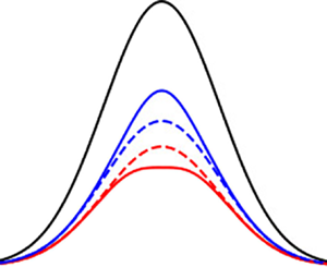
Figure 3 shows a time history of the incident, reflected and transmitted wave amplitudes at the interface for the example case  $n_1/k = 1$ and $\epsilon = \alpha = 0.05$. All terms in the interfacial conditions (3.54) and (3.55) are included, and the results are obtained numerically. The incident wave amplitude at the interface is prescribed by (4.12). Also shown in figure 3, with dashed lines, are the linear reflected and transmitted amplitudes $R_0$ and $T_0$. Figure 3 shows that the reflected amplitude $R$ is less than $R_0$, and the transmitted amplitude $T$ is greater than $T_0$ for all time. This means that for this case, the nonlinear effects make the interface more transparent to internal waves, transmitting more energy and reflecting less than the linear version.

Figure 3. Incident (black), reflected (red) and transmitted (blue) wave amplitudes with  $n_1/k = 1$ and $\epsilon = 0.05$. Dashed lines are the linear amplitudes $R_0$ and $T_0$. The incident wave packet profile is Gaussian.
Figure 4 also shows a time history of the wave amplitudes at  $n_1/k = 1$, but with $\epsilon = \alpha = 0.1$, larger than previously. When $I$ is maximum (at $t = 0$), the profile of $R$ is significantly less than the profile of $R_0$, while $T$ is larger than $T_0$, indicating that the interface is more transparent, as before. For times $t > 0$, after the maximum of $I$ has appeared, both $R$ and $T$ in figure 4 show complex behaviour. This complex behaviour is due to the higher-order linear terms, as in the linear results in figure 2. The value of $\epsilon$ for the results in figure 4 is smaller ( $\epsilon = 0.1$) than in figure 2 ( $\epsilon = 0.5$), and a simulation without the nonlinear terms with $\epsilon = 0.1$ does not show significant homogeneous oscillations. Thus these erroneous homogeneous oscillations are also problematic in the numerical solution to the nonlinear equations, if higher-order linear terms are included.

Figure 4. Incident (black), reflected (red) and transmitted (blue) wave amplitudes with  $n_1/k = 1$ and $\epsilon = 0.1$. Dashed lines are the linear amplitudes $R_0$ and $T_0$. The incident wave packet profile is Gaussian.
The values of  $|R|$ and $|T|$ in figure 4 are seen to be non-zero beyond the time when $I$ has become negligibly small. As with the linear simulations that include higher-order linear effects, these oscillations in the nonlinear equations appear to continue indefinitely, and would cause waves to radiate away from the interface in both layers. While it may be possible for the interface to absorb energy due to nonlinear effects and then radiate energy after $I$ is zero, such radiation cannot continue indefinitely. Thus physically meaningful solutions with larger values of $\epsilon$ (short wave packets) must have the homogeneous oscillations suppressed, most easily achieved simply by neglecting the higher-order linear terms in (3.54) and (3.55).
Figure 5 shows results for the nonlinear case without higher-order linear effects with  $k = 1$ and $\epsilon = 0.1$, the same parameter values as in figure 4. After the incident wave packet in figure 5 is gone, both $R$ and $T$ also are approximately zero. Thus there are no lingering oscillations when the higher-order linear terms are neglected.

Figure 5. Incident (black), reflected (red) and transmitted (blue) wave amplitudes with  $n_1/k = 1$ and $\epsilon = 0.1$. Dashed lines are the linear amplitudes $R_0$ and $T_0$. Nonlinear effects are included, but higher-order linear effects are neglected. The incident wave packet profile is Gaussian.
When the higher-order linear terms are neglected, the instability discussed above is not present, and  $R$ and $T$ may be determined for any small value of $n_1/k$. However, the nonlinear algebraic interfacial conditions do not have roots if the value of $\alpha$ is too large, depending also on the value of $n_1/k$. Figure 6 shows the value of $\epsilon$ above which the numerical iteration does not find any solutions. Also shown in figure 6 are parameter values for the cases of figures 3, 4 and 5.


The numerical results show that nonlinear effects cause a reduction in wave reflection and a corresponding increase in wave transmission. This conclusion is true for all parameter values considered. Thus the interface is more transparent than predicted by linear theory. This is indicated in figure 7, which shows the maximum values of  $R$ and $T$ for an interval of $n_1/k$ with $\epsilon = 0.05$. The maximum values of $R$ and $T$ occur when $I$ is also maximum, and the data in figure 7 correspond to maximum $I$. For all parameter values, $|R| < |R_0|$ and $|T| > |T_0|$. Furthermore, larger values of $n_1/k$ show a larger increase in $|T|$ and decrease in $|R|$ compared to linear values. This same trend with $n_1/k$ is found with all other values of $\epsilon$.

Figure 7. Maximum reflected (red) and transmitted (blue) wave amplitudes with  $\epsilon = 0.05$ over an interval of $n_1/k$. Dashed lines are corresponding maximum values of the linear amplitudes $R_0$ and $T_0$. Nonlinear effects are included, but higher-order linear effects are neglected. The incident wave packet profile is Gaussian.
The interface becomes more transparent to internal waves as  $\epsilon$ increases. This is shown in figure 8 for $n_1/k = 0.4$ and in figure 9 for $n_1/k = 1$. Both figures show the maximum values of $|R|$ and $|T|$, as well as the maxima of $|R_0|$ and $|T_0|$. Clearly, $|R| < |R_0|$ and $|T| > |T_0|$ for all values of $\epsilon$ in both figures, indicating a decrease in reflection and increase in transmission with increasing $\epsilon$. There are no results in figure 9 beyond $\epsilon \approx 0.11$. The nonlinear interfacial conditions do not have roots beyond this value, as indicated in figure 6.

Figure 8. Maximum reflected (red) and transmitted (blue) wave amplitudes with  $n_1/k = 0.4$ over an interval of $\epsilon$. The maximum value for convergence with $n_1/k = 0.4$ is $\epsilon =0.23$. Dashed lines are corresponding maximum values of the linear amplitudes $R_0$ and $T_0$. Nonlinear effects are included, but higher-order linear effects are neglected. The incident wave packet profile is Gaussian.

Figure 9. Maximum reflected (red) and transmitted (blue) wave amplitudes with  $n_1/k = 1$ over an interval of $\epsilon$. The maximum value for convergence with $n_1/k = 1$ is $\epsilon = 0.11$. Dashed lines are corresponding maximum values of the linear amplitudes $R_0$ and $T_0$. Nonlinear effects are included, but higher-order linear effects are neglected. The incident wave packet profile is Gaussian.
Not all nonlinear terms contribute significantly to the reflected and transmitted wave amplitudes. The strongest contributions,  $S_d$, $M_d$ and $M_k$, are plotted in figure 10 for the example case $n_1/k = \sqrt {2}$, $\epsilon = 0.05$ and $N_2/N_1 = 2$. The quantity $S_d$ is the interaction of the secondary harmonic with the primary harmonic in the dynamic condition, and can be seen to have the largest value for all times. The value of $S_d$ is largest for $n_1/k > 0.6$, approximately. For smaller values of $n_1/k$, the interaction between the wave-induced mean and the primary harmonic $M_d$ is largest. The other contributions, $S_k$, $C_k$ and $C_d$ (not shown in figure 10) remain smaller than 10 % of the maximum contributor for all $n_1/k$. This suggests a simpler model for the interfacial conditions, where $S_d$ and/or $M_d$ are retained and the other terms are neglected.

Figure 10. Profile of nonlinear contributions  $M_k$, $M_d$ and $S_d$ for $n_1/k = \sqrt {2}$, $\epsilon = 0.05$ and $N_2/N_1 = 2$. The incident wave packet profile is Gaussian.
6. Conclusions
Internal waves impinging on the abrupt change in buoyancy frequency at the tropopause will reflect partially. Previous theories have treated the reflection using linear interfacial conditions, resulting in the equivalent of Snell's law. Reflection of internal waves is treated here with nonlinear interfacial conditions. The configuration is two layers of stratified Boussinesq fluid, each with a constant but different value of the buoyancy frequency. The density is continuous at the interface of the two layers, but the buoyancy frequency is discontinuous.
The waves are assumed periodic in the horizontal and are confined to a vertical wave packet. The wave amplitude is small, and the wave packet is long. The amplitude equation governing the waves in each layer is the nonlinear Schrödinger equation. The interfacial conditions are expanded to third order, matching the accuracy of the amplitude equations. The interfacial conditions include higher-order terms that are linear in the wave amplitudes as well as terms that include products of the incident, reflected and transmitted wave amplitudes. The higher-order linear terms allow homogeneous oscillations to exist. For steep waves, the homogeneous solution indicates that the waves are unstable at the interface. If the waves are not steep, then the homogeneous oscillations, which should be zero, are negligible if the wave packet is long. However, for short packets, the numerical solution erroneously shows larger homogeneous oscillations. Shorter packets are treated by neglecting the higher-order linear terms while retaining the nonlinear terms.
Results are obtained by dictating the packet shape of the incident wave amplitude at the interface. Both the Gaussian and ‘raised cosine’ profiles are treated. The nonlinear interfacial conditions are treated numerically, producing a time history of reflected and transmitted wave amplitudes at the interface, driven by the time history of the incident wave amplitude at the interface. Results show that the nonlinear effect causes the reflected wave amplitude to be less than the linear value, and the transmitted wave amplitude to be greater than linear. Thus the interface is more transparent to internal waves than predicted by linear theory. Furthermore, the interface is increasingly more transparent with larger amplitude waves, and as the waves become less steep.
Declaration of interests
The author reports no conflict of interest.
Appendix A. Numerical techniques
First transform (3.54) and (3.55) into standard form. Use
 \begin{equation} \left.\begin{gathered} u_1 ={-} {\rm i} ( n_1 + n_2 ) R + {\rm i} ( n_1 - n_2 ) I,\\ u_2 = {\rm i} ( b_1 + b_2 ) R_t - {\rm i} ( b_1 - b_2 ) I_t \end{gathered}\right\} \end{equation}
for (3.54), and
 \begin{equation} \left.\begin{gathered} u_1 ={-} {\rm i} ( n_1 + n_2 ) T + {\rm i} 2 n_1 I,\\ u_2 = {\rm i} ( b_1 + b_2 ) T_t - {\rm i} 2 b_1 I_t \end{gathered}\right\} \end{equation}
for (3.55). In both cases, the result is two first-order equations:
 \begin{align} {u_1}_t &={-} \left[ \frac{n_1 + n_2}{b_1 + b_2} \right] u_2 - {\rm i} \left[ \frac{(b_1 - b_2)(n_1 + n_2) -(b_1 + b_2)(n_1 - n_2)} {b_1 + b_2} \right] I_t, \end{align}
 \begin{align} {u_2}_t &={-} u_1+ {\rm i} \left[ \frac{a_1 + a_2}{b_1 + b_2} \right] u_2 \nonumber\\ &\quad + \frac{1}{(n_1 + n_2)(b_1 + b_2)} [(b_1 + b_2)[(a_1 - a_2)(n_1 + n_2) - (a_1 + a_2)(n_1 - n_2)]\nonumber\\ &\quad - (a_1 + a_2)[(b_1 - b_2)(n_1 + n_2)- (b_1 + b_2)(n_1 - n_2)]]\,I_t\nonumber\\ &\quad + \alpha^2 Q, \end{align}
where  $Q$ represents the pertinent nonlinear terms, namely either $Q_R$ or $Q_T$ depending on whether (3.54) or (3.55) is being treated, respectively. Furthermore, let
 \begin{equation} v_1 = u_1 + {\rm i} \left[ \frac{(b_1 - b_2)(n_1 + n_2) - (b_1 + b_2)(n_1 - n_2)} {b_1 + b_2} \right] I, \end{equation}
 \begin{align} v_2 &= u_2 - \frac{1}{(n_1
+ n_2)(b_1 + b_2)}\, [(b_1 + b_2)[(a_1 - a_2)(n_1 +
n_2) - (a_1 +a_2)(n_1 - n_2)]\nonumber\\ &\quad - (a_1 +
a_2)[(b_1 - b_2)(n_1 + n_2)- (b_1 + b_2)(n_1 - n_2)]]\,I,
\end{align}
\begin{align} v_2 &= u_2 - \frac{1}{(n_1
+ n_2)(b_1 + b_2)}\, [(b_1 + b_2)[(a_1 - a_2)(n_1 +
n_2) - (a_1 +a_2)(n_1 - n_2)]\nonumber\\ &\quad - (a_1 +
a_2)[(b_1 - b_2)(n_1 + n_2)- (b_1 + b_2)(n_1 - n_2)]]\,I,
\end{align}
to get
 \begin{gather} {v_1}_t ={-} c_1 v_2 - d_1 I, \end{gather}
 \begin{gather}{v_2}_t ={-} v_1 + {\rm i} c_2 v_2 + {\rm i} d_2 I + \alpha^2 Q, \end{gather}
where
 \begin{equation} \left.\begin{gathered} c_1 = \frac{n_1 + n_2}{b_1 + b_2},\\ c_2 = \frac{a_1 + a_2}{b_1 + b_2}, \end{gathered}\right\} \end{equation}
 \begin{align} d_1 &= \frac{1}{(b_1 +
b_2)^2}\,[(b_1 + b_2) [ (a_1 - a_2)(n_1 + n_2) - (a_1
+ a_2)(n_1 - n_2) ]\nonumber\\ &\quad
-(a_1 + a_2) [ (b_1 - b_2)(n_1 + n_2) - (b_1 +
b_2)(n_1 - n_2) ]],
\end{align}
\begin{align} d_1 &= \frac{1}{(b_1 +
b_2)^2}\,[(b_1 + b_2) [ (a_1 - a_2)(n_1 + n_2) - (a_1
+ a_2)(n_1 - n_2) ]\nonumber\\ &\quad
-(a_1 + a_2) [ (b_1 - b_2)(n_1 + n_2) - (b_1 +
b_2)(n_1 - n_2) ]],
\end{align}
 \begin{align} d_2 &= \frac{1}{(b_1 +
b_2)^2 (n_1 + n_2)}\, [(a_1 + a_2)(b_1 + b_2) [ (a_1 -
a_2)(n_1 + n_2) \nonumber\\ &\quad
- (a_1 + a_2)(n_1 - n_2) ] \nonumber\\ &\quad -
(a_1 + a_2)^2 [ (b_1 - b_2)(n_1 + n_2) - (b_1 + b_2)(n_1 -
n_2) ]\nonumber\\ &\quad + (b_1 + b_2)(n_1 + n_2)
[ (b_1 - b_2)(n_1 + n_2) - (b_1 + b_2)(n_1 - n_2) ] ]. \end{align}
\begin{align} d_2 &= \frac{1}{(b_1 +
b_2)^2 (n_1 + n_2)}\, [(a_1 + a_2)(b_1 + b_2) [ (a_1 -
a_2)(n_1 + n_2) \nonumber\\ &\quad
- (a_1 + a_2)(n_1 - n_2) ] \nonumber\\ &\quad -
(a_1 + a_2)^2 [ (b_1 - b_2)(n_1 + n_2) - (b_1 + b_2)(n_1 -
n_2) ]\nonumber\\ &\quad + (b_1 + b_2)(n_1 + n_2)
[ (b_1 - b_2)(n_1 + n_2) - (b_1 + b_2)(n_1 - n_2) ] ]. \end{align}
This is more convenient for computations as derivatives of  $I$ are avoided.
The interfacial conditions are integrated numerically using the second-order Adams–Bashforth and Adams–Moulton methods:
 \begin{equation} v_1^{n+1} - v_1^n ={-} c_1 \tfrac{1}{2} ( 3 v_2^n - v_2^{n-1} ) \Delta t - d_1 \tfrac{1}{2} ( I^{n+1} + I^n ) \Delta t, \end{equation}
 \begin{align} v_2^{n+1} - v_2^n &={-}
\tfrac{1}{2}( v_1^{n+1} + v_1^n ) \Delta t + {\rm i} c_2 \tfrac{1}{2} ( 3 v_2^n - v_2^{n-1} )
\Delta t\nonumber\\ &\quad + {\rm i} d_2 \tfrac{1}{2}
left( I^{n+1} + I^n ) \Delta t + \alpha^2 \tfrac{1}{2} ( 3 Q^n - Q^{n-1} ) \Delta t,
\end{align}
\begin{align} v_2^{n+1} - v_2^n &={-}
\tfrac{1}{2}( v_1^{n+1} + v_1^n ) \Delta t + {\rm i} c_2 \tfrac{1}{2} ( 3 v_2^n - v_2^{n-1} )
\Delta t\nonumber\\ &\quad + {\rm i} d_2 \tfrac{1}{2}
left( I^{n+1} + I^n ) \Delta t + \alpha^2 \tfrac{1}{2} ( 3 Q^n - Q^{n-1} ) \Delta t,
\end{align}
where again  $Q$ is either $Q_R$ or $Q_T$. There are two sets of values of $v_1, v_2$, one for $R$ and the other for $T$. For the set leading to the new $R$ value, (A12) is used to obtain $v_1^{n+1}$, then (A13) is used to obtain $v_2^{n+1}$ using $Q = Q_R$. Then finally, $R$ is obtained with
 \begin{align} R^{n+1} &= {\rm i}\,\frac{1}{n_1 + n_2}\,v_1^{n+1} \nonumber\\ &\quad + \left[ \frac{(b_1 - b_2)(n_1 + n_2) - (b_1 + b_2)(n_1 - n_2)} {(n_1 + n_2)(b_1 + b_2)}+ \frac{n_1 - n_2}{n_1 + n_2} \right] I^{n+1}. \end{align}
 The process is repeated with the other set using  $Q = Q_T$, then $T$ is obtained with
 \begin{align} T^{n+1} &= {\rm i}\,\frac{1}{n_1 + n_2}\,v_1^{n+1} \nonumber\\ &\quad + \left[ \frac{(b_1 - b_2)(n_1 + n_2) - (b_1 + b_2)(n_1 - n_2)} {(n_1 + n_2)(b_1 + b_2)}+ \frac{2 n_1}{n_1 + n_2} \right] I^{n+1}. \end{align}
Further accuracy is achieved with iteration. The new values of  $R$ and $T$ are used in the nonlinear terms $Q_R$ and $Q_T$, which are then used to replace the previous values of $Q^n$, allowing improved values of $R$ and $T$ to be determined. This process is repeated until convergence. Ten iterations are found to be adequate.


