


1. Introduction
Demand for land is continuously rising globally (Foley et al., Reference Foley, DeFries, Asner, Barford, Bonan, Carpenter, Chapin, Coe, Daily, Gibbs, Helkowski, Holloway, Howard, Kucharik, Monfreda, Patz, Prentice, Ramankutty and Snyder2005). This is characterized by both intensification and extensification of food production (FAO, 2014), by urbanization (Seto et al., Reference Seto, Güneralp and Hutyra2012), by the onset of modern bioenergy (Chum et al., Reference Chum, Faaij, Moreira, Berndes, Dhamija, Dong, Gabrielle, Goss Eng, Lucht, Mapako, Masera Cerutti, McIntyre, Minowa, Pingoud, Edenhofer, Pichs-Madruga, Sokona, Seyboth, Matschoss, Kadner, Zwickel, Eickemeier, Hansen, Schlömer and von Stechow2011; Creutzig et al., Reference Creutzig, Ravindranath, Berndes, Bolwig, Bright, Cherubini, Chum, Corbera, Delucchi and Faaij2015), by preservation of nature and biodiversity (Wilson, Reference Wilson2016) and, more recently, by afforestation to sequester CO2 on land (Canadell & Raupach, Reference Canadell and Raupach2008). Projected latent land demand, added up from individual studies, could exceed available land by a factor of 3–7 by 2050 (Canadell & Schulze, Reference Canadell and Schulze2014). Even when accounting for plausible multi-purpose allocation, this future demand is unlikely to be matched by available land resources (Davis et al., Reference Davis, Gephart, Emery, Leach, Galloway and D'Odorico2016), raising normative and ethical questions (Risse, Reference Risse2008; Creutzig, Reference Creutzig2017). While a few studies have investigated total area demands for various purposes and have provided long-term outlooks (Smith et al., Reference Smith, Gregory, Van Vuuren, Obersteiner, Havlík, Rounsevell, Woods, Stehfest and Bellarby2010; Hurtt et al., Reference Hurtt, Chini, Frolking, Betts, Feddema, Fischer, Fisk, Hibbard, Houghton and Janetos2011; Lambin & Meyfroidt, Reference Lambin and Meyfroidt2011), a holistic understanding of geographical patterns of the most recent land system dynamics with respect to location and density of land-use changes for human needs (food, shelter) and biophysical stability (biodiversity, climate stabilization) across scales is missing.
Land-use change has been associated with human activities for millennia and, prior to industrialization, was dominated by deforestation induced by population pressure and corresponding demand for cropland, closely following the ascent and descent of civilizations (Kaplan et al., Reference Kaplan, Krumhardt and Zimmermann2009). With the industrialization, fossil fuel substituted for wood fuel, and the nexus between population pressure and deforestation was broken, at least regionally (Krausmann et al., Reference Krausmann, Schandl and Sieferle2008). However, current trends indicate that the re-transition to more land-use intensive economies may exceed global biophysical limits (Rockström et al., Reference Rockström, Steffen, Noone, Persson, Chapin, Lambin, Lenton, Scheffer, Folke, Schellnhuber, Nykvist, de Wit, Hughes, van der Leeuw, Rodhe, Sörlin, Snyder, Costanza, Svedin, Falkenmark, Karlberg, Corell, Fabry, Hansen, Walker, Liverman, Richardson, Crutzen and Foley2009; Steffen et al., Reference Steffen, Richardson, Rockström, Cornell, Fetzer, Bennett, Biggs, Carpenter, de Vries, de Wit, Folke, Gerten, Heinke, Mace, Persson, Ramanathan, Reyers and Sörlin2015). First, at the current rate of technological change, croplands may need to increase by 10–25% by 2050 to feed a growing and more affluent population demanding more land-intensive nutrition (Schmitz et al., Reference Schmitz, van Meijl, Kyle, Nelson, Fujimori, Gurgel, Havlik, Heyhoe, d'Croz, Popp, Sands, Tabeau, van der Mensbrugghe, von Lampe, Wise, Blanc, Hasegawa, Kavallari and Valin2014). Second, human settlements expand, demanding an unprecedented area of land that is on average about twice as agriculturally productive as world average cropland (Bren d'Amour et al., Reference Bren d'Amour, Reitsma, Baiocchi, Barthel, Güneralp, Erb, Haberl, Creutzig and Seto2017). Third, energy production has started to shift back from fossil- to land-intensive fuels, a development potentially desirable to reduce counterfactual greenhouse gas emissions (Creutzig et al., Reference Creutzig, Ravindranath, Berndes, Bolwig, Bright, Cherubini, Chum, Corbera, Delucchi and Faaij2015) or to even generate so-called negative emissions (Fuss et al., Reference Fuss, Canadell, Peters, Tavoni, Andrew, Ciais, Jackson, Jones, Kraxner and Nakicenovic2014; Smith et al., Reference Smith, Davis, Creutzig, Fuss, Minx, Gabrielle, Kato, Jackson, Cowie, Kriegler, van Vuuren, Rogelj, Ciais, Milne, Canadell, McCollum, Peters, Andrew, Krey, Shrestha, Friedlingstein, Gasser, Grübler, Heidug, Jonas, Jones, Kraxner, Littleton, Lowe, Moreira, Nakicenovic, Obersteiner, Patwardhan, Rogner, Rubin, Sharifi, Torvanger, Yamagata, Edmonds and Yongsung2016). Fourth, land could provide the space for an enhanced terrestrial carbon sink, for example, by afforestation, thus contributing to the mitigation of climate change (Minx et al., Reference Minx, Lamb, Callaghan, Fuss, Hilaire, Lenzi, Nemet, Creutzig, Amann, Beringer, de Oliveira Garcia, Hartmann, Khanna, Luderer, Nemet, Rogelj, Rogers, Smith and del Mar Zamora2018). Fifth, ecosystems need to be stabilized across the globe to avoid unprecedented human-made biodiversity loss (Newbold et al., Reference Newbold, Hudson, Hill, Contu, Lysenko, Senior, Börger, Bennett, Choimes and Collen2015). As decision-makers become aware of climate change and biodiversity concerns, previously low-value residual land increases in value, limiting the availability for other purposes. At the same time, anthropogenic climate change itself affects the ‘supply side’ of land use, for example, by changing temperature and precipitation patterns or CO2 fertilization, in part reducing crop yields (Lobell, Reference Lobell2011), especially at higher levels of warming and at lower latitudes affecting developing countries most (Rosenzweig et al., Reference Rosenzweig, Elliott, Deryng, Ruane, Müller, Arneth, Boote, Folberth, Glotter, Khabarov, Neumann, Piontek, Pugh, Schmid, Stehfest, Yang and Jones2014). In short, developing human land pressures encounter global biophysical constraints and threaten global commons, such as biodiversity and climate.
This paper investigates global land-use change for different purposes and perspectives between 2000 and 2010 with harmonized metrics. It investigates effects of direct and telecoupled land demand (defined as socioeconomic and environmental interaction over long distances, including trade and climate change (Liu et al., Reference Liu, Hull, Batistella, DeFries, Dietz, Fu, Hertel, Izaurralde, Lambin, Li, Martinelli, McConnell, Moran, Naylor, Ouyang, Polenske, Reenberg, de Miranda Rocha, Simmons, Verburg, Vitousek, Zhang and Zhu2013)) presenting a comprehensive, but spatially and regionally differentiated picture of global demand for land. Rather than providing a synthesis of existing land cover change data sets (Lepers et al., Reference Lepers, Lambin, Janetos, DeFries, Achard, Ramankutty and Scholes2005), this paper uses a range of data sets to map and hence visualize land-use changes and validate the findings with a region-specific literature review. Land-use changes have been previously and comprehensively studied, even on century-long time scales (Lambin & Geist, Reference Lambin and Geist2008). Here we focus on assessing land-use changes between 2000 and 2010 and pose the following questions:
• How did land use change for population, livestock, cropland, carbon and biodiversity between 2000 and 2010? We map and evaluate land-use changes at 50 × 50 km resolution in terms of changes of density in land use (e.g. change in population density).
• Did land use change more in regimes of high or low use densities? We graphically evaluate changes in land use for different density regimes.
• Where did what kind of land-use changes occur simultaneously? We statistically evaluate spatial co-occurrences globally, and for ten different world regions, and perform a principal component analysis on co-occurring land-use changes.
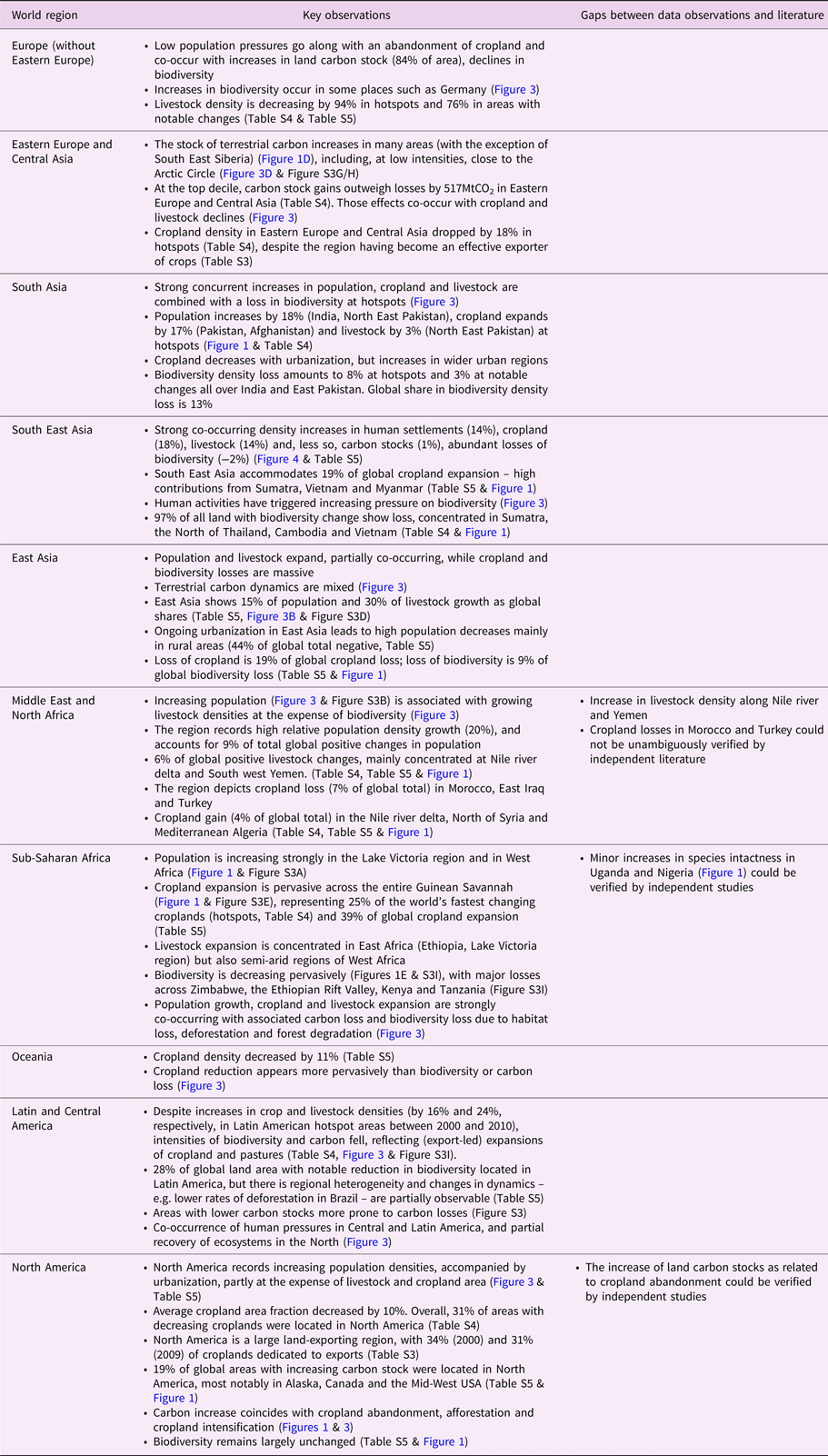
• What are the underlying land-use change dynamics? We perform a world-region specific and systematic literature review to interpret the observed land-use changes, and develop a typology of land-use change patterns across world regions.
This assessment is relevant in that there is an emerging class of global land assessments, including the Global Land Outlook (UNCCD, 2017), the upcoming IPBES Global Assessment, and the upcoming IPCC's special report on climate change, desertification, land degradation, sustainable land management, food security, and greenhouse gas fluxes in terrestrial ecosystems (SRCCL). It is our intention to provide input and background to these assessment processes.
2. Methods and data
The data analysis makes use of the highest quality data available for 2000–2010 (see Table 1 for an overview). In the following we explain data, data processing, their limitations and computational methods chosen.
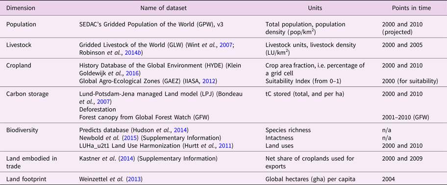
Table 1. Overview of datasets. Data selection was based on quality and availability for the years 2000 and 2010. Modelled data is only used if alternatives were unavailable. See Supplementary Information for more details.
2.1. Data and data processing
This study combines gridded datasets of different land-use dimensions and their respective intensities. Data selection is based on quality and availability for the year 2000 and 2010. All data are processed and mapped into a 30 arc-minute (0.5 degree) grid, corresponding to ≈50 × 50 km at equator, and finer resolution at higher latitudes. The sample size ensures statistically relevant measurements of co-occurrences of land-use change and statistical analysis on a world region scale. All data were read in, re-sampled (if applicable), and compiled into a single dataset for subsequent analysis, using zonal statistics in ArcGIS.
Additional processing steps were required for the data used in livestock and biodiversity dimensions as well as for carbon:
2.2. Livestock data
Livestock datasets of the most important livestock types (poultry, pigs, goats, sheep and cattle) were read in as layers and re-sampled to 2.5’ arc minute. The aggregate Livestock Unit (LU) Layer was generated with the raster calculator tool using the Livestock Layers and Livestock Unit Conversion Factors (poultry: 0.01, pigs: 0.225, goats: 0.1, sheep: 0.1 and cattle: 0.7; derived from http://www.lrrd.org/lrrd18/8/chil18117.htm).
2.3. Biodiversity data
Biodiversity is defined as the stock of plants (including trees) and animals (including fish), fungi and bacteria (e.g. for food, fuels, fibre and medicine, genetic resources for developing new crops or medicines, or as a tourism asset, etc.) following the official SEEA (System of Environmental Economic Accounting) definition (United Nations, 2014). The focus of our study is terrestrial biodiversity, thus including fish (in rivers, lakes, etc.), but not offshore marine life. We use the map of species richness by UNEP/WCMC, which covers the taxonomic groups of birds, mammals and amphibians, based on the PREDICTS project (Hudson et al., Reference Hudson, Newbold, Contu, Hill, Lysenko, De Palma, Phillips, Senior, Bennett, Booth, Choimes, Correia, Day, Echeverría-Londoño, Garon, Harrison, Ingram, Jung, Kemp, Kirkpatrick, Martin, Pan, White, Aben, Abrahamczyk, Adum, Aguilar-Barquero, Aizen, Ancrenaz, Arbeláez-Cortés, Armbrecht, Azhar, Azpiroz, Baeten, Báldi, Banks, Barlow, Batáry, Bates, Bayne, Beja, Berg, Berry, Bicknell, Bihn, Böhning-Gaese, Boekhout, Boutin, Bouyer, Brearley, Brito, Brunet, Buczkowski, Buscardo, Cabra-García, Calviño-Cancela, Cameron, Cancello, Carrijo, Carvalho, Castro, Castro-Luna, Cerda, Cerezo, Chauvat, Clarke, Cleary, Connop, D'Aniello, da Silva, Darvill, Dauber, Dejean, Diekötter, Dominguez-Haydar, Dormann, Dumont, Dures, Dynesius, Edenius, Elek, Entling, Farwig, Fayle, Felicioli, Felton, Ficetola, Filgueiras, Fonte, Fraser, Fukuda, Furlani, Ganzhorn, Garden, Gheler-Costa, Giordani, Giordano, Gottschalk, Goulson, Gove, Grogan, Hanley, Hanson, Hashim, Hawes, Hébert, Helden, Henden, Hernández, Herzog, Higuera-Diaz, Hilje, Horgan, Horváth, Hylander, Isaacs-Cubides, Ishitani, Jacobs, Jaramillo, Jauker, Jonsell, Jung, Kapoor, Kati, Katovai, Kessler, Knop, Kolb, Kőrösi, Lachat, Lantschner, Le Féon, LeBuhn, Légaré, Letcher, Littlewood, López-Quintero, Louhaichi, Lövei, Lucas-Borja, Luja, Maeto, Magura, Mallari, Marin-Spiotta, Marshall, Martínez, Mayfield, Mikusinski, Milder, Miller, Morales, Muchane, Muchane, Naidoo, Nakamura, Naoe, Nates-Parra, Navarrete Gutierrez, Neuschulz, Noreika, Norfolk, Noriega, Nöske, O'Dea, Oduro, Ofori-Boateng, Oke, Osgathorpe, Paritsis, Parra-H, Pelegrin, Peres, Persson, Petanidou, Phalan, Philips, Poveda, Power, Presley, Proença, Quaranta, Quintero, Redpath-Downing, Reid, Reis, Ribeiro, Richardson, Richardson, Robles, Römbke, Romero-Duque, Rosselli, Rossiter, Roulston, Rousseau, Sadler, Sáfián, Saldaña-Vázquez, Samnegård, Schüepp, Schweiger, Sedlock, Shahabuddin, Sheil, Silva, Slade, Smith-Pardo, Sodhi, Somarriba, Sosa, Stout, Struebig, Sung, Threlfall, Tonietto, Tóthmérész, Tscharntke, Turner, Tylianakis, Vanbergen, Vassilev, Verboven, Vergara, Vergara, Verhulst, Walker, Wang, Watling, Wells, Williams, Willig, Woinarski, Wolf, Woodcock, Yu, Zaitsev, Collen, Ewers, Mace, Purves, Scharlemann and Purvis2014). PREDICTS has collated a large dataset from published studies on how biodiversity responds to human impacts, particularly land use. It extrapolates diversity metrics such as species richness across spatial scales using global and regional statistical models. That is especially true in regions with fewer data points, such as Sub-Saharan Africa (SSA), which to a large extent depends on extrapolated data. Species richness can be interpreted as the potential number of different species in one grid cell, thus measuring actual diversity and not absolute numbers. From species richness, we compute ‘intactness’ as proxy for the biodiversity dimension. The intactness of a grid cell is an index of how much of the initial species richness of a grid cell (untouched, i.e. in 100% ‘primary’ vegetation) is impacted by other land uses (road construction and pasture expansion are explicitly considered, among others). The intactness for a given year is computed by factoring in gridded land-use data (for both 2000 and 2010). We use land-use information from the ‘Land-Use Harmonization 2’ project (Hurtt et al., Reference Hurtt, Chini, Frolking, Betts, Feddema, Fischer, Fisk, Hibbard, Houghton and Janetos2011) (version LUH2 v2 h), which uses agriculture and urban land-use data from HYDE 3.2 (Klein Goldewijk et al., Reference Klein Goldewijk, Beusen, Doelman and Stehfest2016) and other land-use information to create annual maps of human land use. Every land-use type in a grid cell (in fractions of a grid cell) gets assigned a different impact on the original, initial species richness in that cell, methodologically following Newbold et al. (Reference Newbold, Hudson, Hill, Contu, Lysenko, Senior, Börger, Bennett, Choimes and Collen2015) (see Supplementary Information, Table S1 in Newbold et al., Reference Newbold, Hudson, Hill, Contu, Lysenko, Senior, Börger, Bennett, Choimes and Collen2015). For instance, Newbold et al. assign cropland (light use) an effect size of 61.9 on species richness, indicating that the intactness of a grid cell containing only cropland is 61.9 compared to 100 under natural primary vegetation. Newbold et al. also differentiate between different intensities of land-use types (minimal, light, intense use) and, in the case of secondary vegetation, different maturities (young, intermediate, mature). These will have an impact on the effect of the land-use type on the species richness. In our calculations, the density of the land-use type is assumed to be light (not minimal or intense). The light density allows for relatively high species richness, independent of the land-use type it is associated with. The resulting estimate can be regarded as relatively conservative since it would be in the lower range of the potential effects on species richness. Using these inputs, the intactness of each grid cell is computed. The resulting intactness is weighted with the species richness of the cell and divided by the corresponding area of the cell. In other words, if intactness is considerably impacted in a region with very low species richness, the intactness density metric will be comparatively low. The resulting biodiversity density metric is intactness weighted by species richness/km2.
2.4. Land carbon data
We use the process-based dynamic global vegetation model LPJmL 3.2 (Sitch et al., Reference Sitch, Smith, Prentice, Arneth, Bondeau, Cramer, Kaplan, Levis, Lucht, Sykes, Thonicke and Venevsky2003; Gerten et al., Reference Gerten, Schaphoff, Haberlandt, Lucht and Sitch2004; Bondeau et al., Reference Bondeau, Smith, Zaehle, Schaphoff, Lucht, Cramer, Gerten, Lotze-Campen, Müller, Reichstein and Smith2007) to estimate land carbon stocks in vegetation and soils. LPJmL is a global, grid-based biogeography–biogeochemistry model, which simulates terrestrial carbon pools and fluxes and the biogeographical distribution of natural vegetation. The representation of agricultural land driven by land-use data allows for the quantification of the impacts of land use on water and carbon cycles. Here we used observation-based monthly temperature and cloud cover time series provided by the Climatic Research Unit (CRU TS version 3.21) (University of East Anglia Climatic Research Unit, Reference Jones and Harris2013; Harris et al., Reference Harris, Jones, Osborn and Lister2014) and monthly gridded precipitation data based on the Global Precipitation Climatology Centre (GPCC) Full Data Reanalysis Version 6.0 (Becker et al., Reference Becker, Finger, Meyer-Christoffer, Rudolf, Schamm, Schneider and Ziese2013). We calculate terrestrial carbon storage as the sum of all above- and below-ground carbon stocks in vegetation and soil.
We use land-use information from the LUH2 v2 h which, as already indicated, includes data from HYDE 3.2. HYDE 3.2 does not directly estimate deforestation, for example, using satellite data time series, and will therefore likely underestimate forest loss (Klein Goldewijk et al., Reference Klein Goldewijk, Beusen, Doelman and Stehfest2016) during our assessment period. This is a serious shortcoming, as the period 2000–2012 witnessed 2.3 million square kilometers of forest loss and 0.8 square kilometers of forest gain (Hansen et al., Reference Hansen, Potapov, Moore, Hancher, Turubanova, Tyukavina, Thau, Stehman, Goetz and Loveland2013). Therefore, we combined the LUH2 data with spatially explicit estimates of recent deforestation from the Global Forest Watch (GFW) project. Following the approach of Zarin et al. (Reference Zarin, Harris, Baccini, Aksenov, Hansen, Azevedo-Ramos, Azevedo, Margono, Alencar, Gabris, Allegretti, Potapov, Farina, Walker, Shevade, Loboda, Turubanova and Tyukavina2016) we use only deforestation data within the tropical latitudes because most recent conversion of natural forest to a new land use occurs within the tropics (FAO, 2016; Gibbs et al., Reference Gibbs, Ruesch, Achard, Clayton, Holmgren, Ramankutty and Foley2010).
We calculated the annual increase of tropical cropland and pastures in each cell of LUH2 and compared these changes to the amount of deforestation observed by GFW. Where GFW observes more deforestation than LUH2 we added the difference between the two to the LUH2 data for LPJmL We used average land-use composition (cropland area and types of crops as well as pasture area) from neighbouring cells, where GFW indicates deforestation but no agricultural areas exist in the cell according to LUH2. We are aware that we directly compare and combine gross deforestation measured by GFW with net deforestation in LUH2, but we believe this is a valid approach to reduce the overall deforestation bias in the underlying HYDE 3.2 data.
2.5. Limitations
Data quality limits the scope of this analysis. Data on vegetation and soil carbon stocks, and cropland suitability are modelled, and the biodiversity data are downscaled proxy data. Estimates of land carbon stock (LPJmL) are uncertain due to modelled CO2 fertilization, and only partially empirically validated for 2010 (see above). LPJmL also relies, inter alia, on HYDE data, and hence is not completely independent of cropland data. Hence, our data analysis is likely to miss some land-use changes dynamics that have occurred between 2000 and 2010. Specifically, this is a major concern in that our data insufficiently reflect deforestation dynamics from 2000 until 2010. To account for this, we include empirical data from GFW for the major deforestation regions, and corrected LPJmL data accordingly (see above).
Data are only partially available for 2010. Specifically, established datasets on livestock (Robinson et al., Reference Robinson, Wint, Conchedda, Boeckel, Ercoli, Palamara, Cinardi, D'Aietti, Hay and Gilbert2014b) only go as far as 2005. Some data (e.g. population, livestock) are based on census data. Not all countries provide frequently updated censuses, therefore some of the estimates are based on a single census year, while others have had adjustments applied to normalize the data from different census years to a common set of boundaries.
The resolution is insufficiently high for reporting shifts in land-use change on identical patches of land. Instead, the analysis reveals co-occurring land-use changes in particular regions, and by this, statistical inference of cross effects.
Data should be taken with care in inter-annual comparisons as changes can result from adjustments or reflections of national or regional growth rates rather than reflecting, for example, net migration or population growth. Hence, differences between the observed points in time, 2000 and 2010, should be seen as indicators rather than fixed values. That is especially true for the modelled data on biodiversity and carbon stocks. Both the biodiversity and the LPJmL model use land-use information from LUH2 v2 h, which draws on HYDE 3.2 data, that is, the same data we use for the cropland dimension. Observed co-occurrences between cropland and the biodiversity and carbon dimensions are hence expected.
The reason for choosing HYDE 3.2 for our cropland dimension lies in its temporal availability and the compatibility. While higher resolution cropland maps à la Ramankutty et al. (Reference Ramankutty, Evan, Monfreda and Foley2008) or Fritz et al. (Reference Fritz, See, McCallum, You, Bun, Moltchanova, Duerauer, Albrecht, Schill, Perger, Havlik, Mosnier, Thornton, Wood-Sichra, Herrero, Becker-Reshef, Justice, Hansen, Gong, Abdel Aziz, Cipriani, Cumani, Cecchi, Conchedda, Ferreira, Gomez, Haffani, Kayitakire, Malanding, Mueller, Newby, Nonguierma, Olusegun, Ortner, Rajak, Rocha, Schepaschenko, Schepaschenko, Terekhov, Tiangwa, Vancutsem, Vintrou, Wenbin, Velde, Dunwoody, Kraxner and Obersteiner2015) are likely to be more accurate, there are trade-offs in terms of temporal availability and compatibility. HYDE 3.2, which was recently upgraded, provides consistent cropland layers for both 2000 and 2010, while the other products are only available for 2000 (Ramankutty et al., Reference Ramankutty, Evan, Monfreda and Foley2008) and 2005 (Fritz et al., Reference Fritz, See, McCallum, You, Bun, Moltchanova, Duerauer, Albrecht, Schill, Perger, Havlik, Mosnier, Thornton, Wood-Sichra, Herrero, Becker-Reshef, Justice, Hansen, Gong, Abdel Aziz, Cipriani, Cumani, Cecchi, Conchedda, Ferreira, Gomez, Haffani, Kayitakire, Malanding, Mueller, Newby, Nonguierma, Olusegun, Ortner, Rajak, Rocha, Schepaschenko, Schepaschenko, Terekhov, Tiangwa, Vancutsem, Vintrou, Wenbin, Velde, Dunwoody, Kraxner and Obersteiner2015). In addition, using cropland products from different sources would raise concerns regarding the compatibility. Fritz et al., for example, have compared their findings to the product from Ramankutty et al. and found that “the size of disagreeing areas between the two products is significantly larger than any change in cropland extent between 2000 and 2005 for the majority of countries” (Fritz et al., 2016). Overall, there are considerable differences between different cropland extent datasets (Anderson et al., Reference Anderson, You, Wood, Wood-Sichra and Wu2015; Fritz et al., Reference Fritz, See, McCallum, You, Bun, Moltchanova, Duerauer, Albrecht, Schill, Perger, Havlik, Mosnier, Thornton, Wood-Sichra, Herrero, Becker-Reshef, Justice, Hansen, Gong, Abdel Aziz, Cipriani, Cumani, Cecchi, Conchedda, Ferreira, Gomez, Haffani, Kayitakire, Malanding, Mueller, Newby, Nonguierma, Olusegun, Ortner, Rajak, Rocha, Schepaschenko, Schepaschenko, Terekhov, Tiangwa, Vancutsem, Vintrou, Wenbin, Velde, Dunwoody, Kraxner and Obersteiner2015).
LPJmL models uncertain CO2 fertilization. However, previous studies indicate that LPJ reproduces the magnitude of observed changes in forest productivity due to rising CO2 concentrations (Hickler et al., Reference Hickler, Smith, Prentice, Mjöfors, Miller, Arneth and Sykes2008). Effects of continuous forest management on vegetation and soil carbon stocks are not included, because spatially explicit, global data on forest management are not available (e.g. small-scale or selective logging). To capture relevant dynamics, we hence consider large area deforestation recorded in the GFW data in the simulations, thus putting our estimates into the right magnitude. This study combines gridded datasets of different land-use dimensions and their respective intensities. It focuses exclusively on land-use dynamics and does not cover water as an additional component, which is beyond the scope of this study. By focusing on a rather limited time period only (2000–2010), more recent dynamics are not captured in our data analysis.
Importantly, while some data points of the image maps might be wrong, all messages reported in the text manuscripts were cross-validated with the systematic review in Table 3 and the associated text.
2.6. Density curves
Density curves are constructed to depict the distribution of the land-use dimensions in terms of area and density. To this end, area (in km2) of grid cells that fall into the respective density bins were aggregated. To measure the spatial concentration of land use we computed the Gini coefficient of the five dimensions.
For most dimensions we use a density metric (including a ‘productivity’ dimension), such as livestock units per unit area. For croplands, the corresponding metric would have been cropland area fraction (the percentage of a unit area/grid cell that is covered by croplands). However, this would not account for quality of the respective cropland, which we consider an essential component in the context of croplands. To account for this, we include the GAEZ cropland suitability index as metric for cropland when calculating the distribution of changes in the density of land use. For the rest of the analysis, we use the cropland area fraction.
2.7. Density change
Density change refers to the respective land-use dimension (Tables S1, S4 & S5) in a grid cell between 2000 and 2010, for example, the change in population density (population/km2) in a grid cell. First, we calculate the density for each land-use dimension. Second, we compute the change for each grid cell between 2000 and 2010. We calculate both relative and absolute density change to identify where and to what extent specific changes occurred, respectively, and how much area was affected and at what magnitude.
2.8. Principle component analysis
Principle component analysis (PCA) was performed using STATA 14 to identify major underlying patterns of land-use changes. The PCA is a statistical technique to reduce the dimensions of large datasets by orthogonal transformations to a lower-dimensional space (Jolliffe, Reference Jolliffe2002). Particularly, we are interested in the first principal component which accounts for the largest variance in the data when considering only one dimension. The first component is the eigenvector of the correlation matrix, which corresponds to the largest eigenvalue. The results are shown in Table S2.
The first component (Figure S1A) indicates that the variables can be grouped into those with positive signs (population density, crop area and livestock density) and with negative signs (carbon, biodiversity). These two groups have a clear interpretation as they correspond to direct human pressures (positive sign) and the nature-related residual (negative sign) which means that categorizing dynamics among this dimension allows to explain the largest share of the variability in the data. Adding additional orthogonal components (e.g. component 2; Figure S1B) would increase explanatory power; the second component is, however, difficult to interpret. We therefore restrict to only the first component, which has high statistical power as well as a clear interpretation.
In order to visualize overall land-use dynamics according to the first principal component (the ‘human-vs-nature’ dimension), the corresponding eigenvector is multiplied with the normalized data. The normalization to zero mean and one standard deviation variance is necessary to convert the different variables and dimensions to one comparable metric. The resulting scores indicate whether overall land-use changes are related to human drivers (high positive score) or to the nature residual (large negative score). As the scores result from the normalized data, they must be interpreted relative to the overall land-use dynamics. Hence, a negative score does not mean that nature-related land-use changes are ‘stronger’ than human-related land-use changes. Rather, large positive and negative values indicate regions where human or natural forces are particularly strong.
For interpretation and in-depth understanding of observed co-occurring global land-use change between 2000 and 2010, we perform an in-depth literature research on regional drivers of land-use dynamics, explaining hotspots and their regional and global relevance (see Supplementary Information and associated online material).
2.9. Land embodied in crop trade
Our detailed spatial analysis focuses on local dynamics. For discussing the results, referring to spatial linkages particularly through trade is useful because trade in agricultural products links local land-use decisions to far-distant or global demand changes. Trade in agricultural products involves implicit trade of the production factors that are used to produce the traded goods. The concept of factors embodied in trade is particularly used for analyzing virtual water trade (Hoekstra & Hung, Reference Hoekstra and Hung2005; Dalin et al., Reference Dalin, Konar, Hanasaki, Rinaldo and Rodriguez-Iturbe2012), carbon emissions embodied in trade (Peters & Hertwich, Reference Peters and Hertwich2008) and, more recently, also for quantifying crop land that is associated with trade (Kastner et al., Reference Kastner, Erb and Haberl2014). Based on bilateral virtual land trade data (Kastner et al., Reference Kastner, Erb and Haberl2014), we calculate in Table S3 the share of the cropland in our world regions that is associated with net exports in the years 2000 and 2009. The Oceania region is, for example, a large land exporter as roughly 70% of the cropland is associated with net exports of crops. Hence, local land-use dynamics can be expected to be strongly influenced by international markets. On the contrary, Sub-Saharan Africa, South Eastern Asia and Southern Asia are largely land self-sufficient. Note that this can be consistent with large food trade flows (as we look only at exports net of imports) and trade deficits or surpluses that are measured in monetary terms and quantities of particular food items (and not land). Finally, Europe, Eastern Asia, the Middle East and North Africa rely on large land imports. For these three regions, dependency on imported land has substantially increased.
2.10. Systematic review
We cross-validated our results – co-occurring land-use change patterns in particular regions and cross effects – with a detailed systematic review of region-specific literature, both in the manuscript and in more detail in the Supplementary Information. The systematic review builds on the query: “land use change” AND “[world region]” AND “2000” AND “2010” excluding publications published before 2011. We read the first 30 publications for each query in Google Scholar in detail. We designed additional targeted queries if our data analysis indicated hotspots of specific issues in some particular region. Observations of our data analysis are systematically summarized in Table 3 and verified by detailed analysis in the systematic review of the Supplementary Information. Table 3 also lists observations, which could not be verified by the systematic literature review.
3. Results
3.1. Mapping change in global land use
We first investigated the change in density of land use for human pressures from population growth, expanding livestock production and croplands, as well as their impacts on the biophysical metrics carbon density and biodiversity (Figure 1 & Table 2). Underlying data sources are in several instances (carbon and biodiversity in particular, see Methods and data section) based on numeric models. The ‘changes’ we describe here hence need to be understood against this background and should mainly be understood as model-based estimates. We validate the model-driven results with (data-driven) literature results in a separate section. We rely on density metrics, here always understood as units (population, livestock unit, cropland area fraction, carbon storage by using tonnes of terrestrial carbon stored and biodiversity intactness weighted by species richness) per area (km2), see Methods and data section. We designated hotspots as areas where 10% of the highest absolute changes in density occur, and notable change areas where 80% of the highest absolute changes in density occur, filtering out land-use change of low magnitudes. When not explicitly described as hotspots, land-use dynamics are represented by notable change areas.
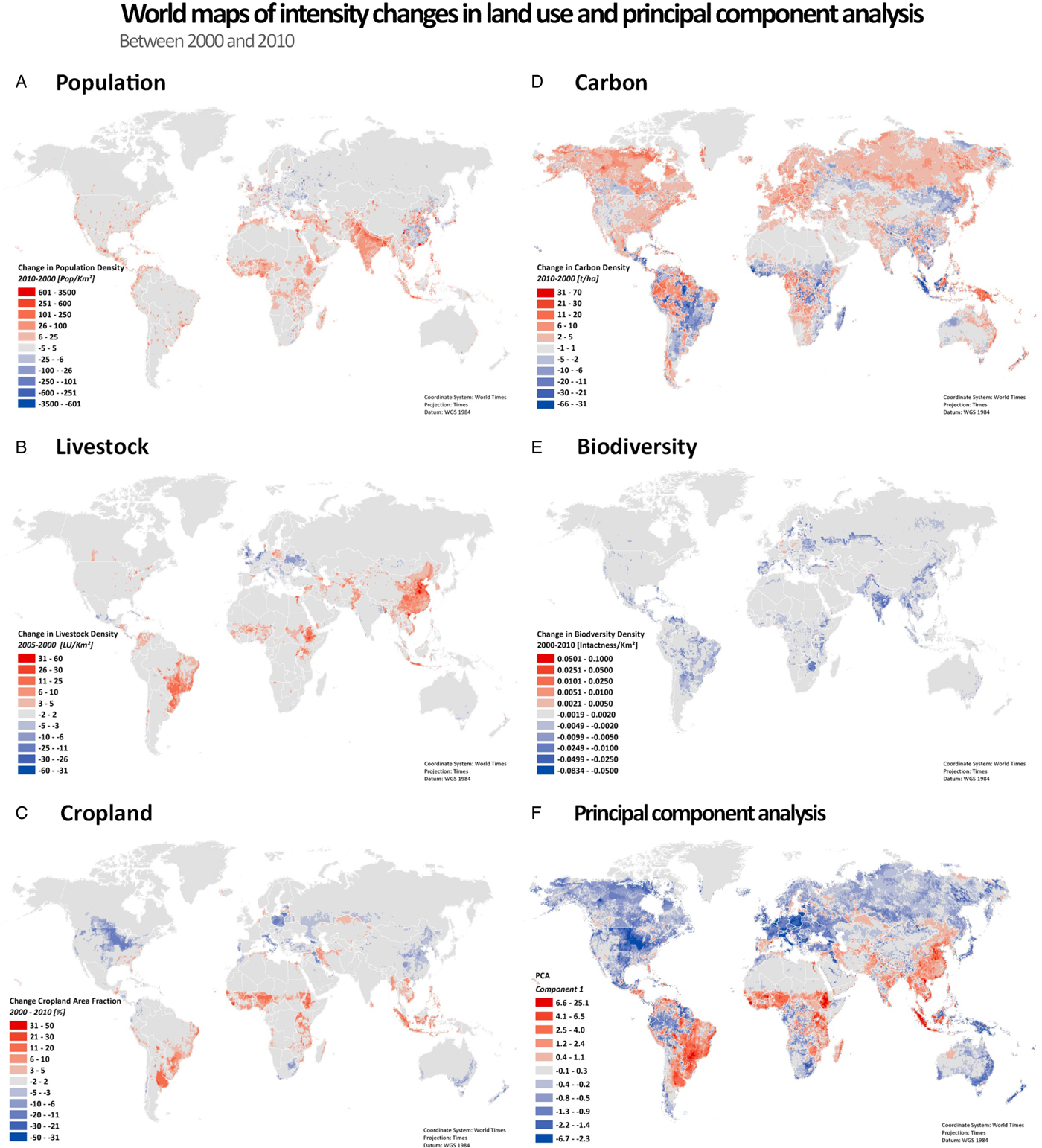
Fig. 1. Change in density of land use between 2000 and 2010. (A) Population density; (B) Livestock density (for 2000 and 2005); (C) Cropland area fraction; (D) Terrestrial carbon density; (E) Biodiversity intactness (proxy for biodiversity); (F) Principal component analysis Z-scores from the product of the first eigenvector with the standardized data of density changes. Blue colors indicate that increases in carbon stocks and biodiversity are relatively strong while red colors indicate that population, cropland and livestock gains dominate (relative to the mean change). All data are processed and mapped into a 30 arc-minute (0.5 degree) grid (63879 data points), corresponding to ≈50 × 50 km at equator, and finer resolution at higher latitudes. Data sources are summarized in Table S1.
Table 2. Gain/loss per land-use dimension with density change above threshold between 2000 and 2010 (2000 and 2005 for livestock).
Density units: 1) Population: population/km2; 2) Livestock: livestock units/km2; 3) Cropland: cropland area fraction (here defined as percentage of cropland in a grid cell); 4) Carbon: tC/ha; 5) Biodiversity: intactness/km2 (weighted with species richness). Intactness measures the degree to which the original biodiversity of a terrestrial site remains unimpaired in the face of human land use and related pressures. Threshold refers to changes in density between 2010 (2005 for livestock) and 2000: Top 10% = hotspot areas of density change; Top 80% = areas with notable changes.
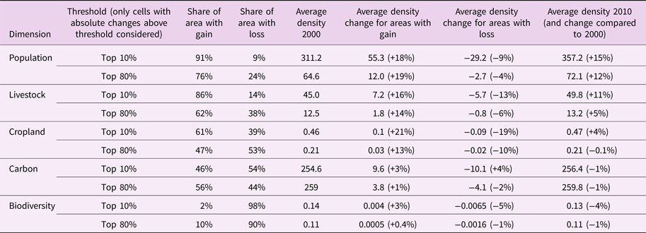
Population density is increasing on 76% of land (within notable change areas), and on 91% of the hotspot areas (Table 2 & Figure 1A). Population density growth is most substantial on the Indian subcontinent, Northern Africa and Western Asia, West Africa, the Lake Victoria region and around the Sao Paolo mega-urban region (Figure 1A). In parts of Eastern Europe, and rural China, population density is decreasing. The cropland area fraction is increasing in hotspot areas (on 61% of hotspot area), but overall, cropland area fraction is decreasing in a slight majority of places (53%; Table 2). Cropland is expanding most prominently in Mato Grosso, Brazil, the Guinean Savannah zone and Sumatra (South East Asia), but is declining across large parts of the Northern hemisphere (Figure 1C). Sub-Saharan Africa is the region showing greatest human pressures as population density increased on average by 27%, and cropland expanded by 18%, between 2000 and 2010 (Table S5). Next to population, the greatest increase is in livestock (on 62% of land). The most notable increases in livestock density appear in China, Brazil and parts of Sub-Saharan Africa, but there are decreases in parts of Europe (Figure 1B). Worldwide, a small majority of places display an increase in land carbon stock (55%), notably in the Northern hemisphere and in tropical rain forests (parts of the Amazon, Congo and Indonesia) (Figure 1D). By contrast, decreases occur in most of South America, Sub-Saharan Africa, Sumatra and some North-American regions (e.g. Alberta). Notably, 57% of global net terrestrial carbon loss took place in Sub-Saharan Africa and Latin America, together with 68% of global net cropland expansion (Table S5). With rare exceptions, biodiversity is decreasing worldwide (90%; and 98% of hotspots).
3.2. Shifts in density of land uses
Changes of land use are concentrated in specific density bands (Figure 2). An analysis of the magnitude of density shift for all land areas reveals that more than 90% of the shifts have an absolute value of <10% of their respective scales as presented in Figure 2; population and livestock shifts tend to be positive, while biodiversity shifts are strongly negative (Figure S2). We cross-validated results from Figure 2 with a world-region specific literature review (Table 3). Remote land becomes more populated, reflecting human land take in sub-Saharan Africa, the Arabian Peninsula and in a few scarcely populated areas of the Americas (Figure 2A, Figure S3A & Table 3). The area of high population concentration (>900 pop/km2) increases, reflecting urbanization in the Bengal delta, coastal China, the Nile delta and Java (Figure 2A, Figure S3B & Table 3). Livestock land area declines exponentially with density: with large areas of land being used for very low-intensive husbandry (Figure 2B). Livestock is increasing in areas of very low density, that is, mostly in Brazil, Northern China, and the Guinean Savannah, but there is less husbandry in Eastern Europe (Figure 2B, Figure S3C & Table 3). Livestock is also increasing in areas of higher density, reflecting industrial livestock breeding in Shandong, Hebei and Henan provinces in China, and around Sao Paulo, Brazil (Figure 1, Figure 2B, Figure S3D & Table 3). There is an expansion of cropland of medium suitability in the Guinean Savannah and South America, but there is a loss of cropland in the USA and Eastern Europe (Figure 2, Figure S3E & Table 3). Land of very high suitability was utilized less for agriculture in the US Mid-West in 2010, while cropland has expanded in the highly suitable Chaco region of Argentina producing soybean for exports (Figure 2C, Figure S3F & Table 3). At the same time, some land of low suitability has been abandoned (Figure 2C). Most of this land has less than 50tC/ha carbon stock, which is low compared to the peak value of 1850tC/ha (Keith et al., Reference Keith, Mackey and Lindenmayer2009) (Figure 2D). The change in density of terrestrial carbon is complex, but there is a distinct increase in carbon stored by land at <100tC/ha, particularly close to the Arctic Circle (Figure 2D & Figure S3G). There is also an increase of terrestrial carbon stored at around 400tC/ha in boreal areas and in the tropics (Figure 2D, Figure S3H & Table 3). Areas of medium–high species intactness are lost, particularly in South Asia (India and Pakistan) and the Chaco region, Argentina (Figure 2E, Figure S3I & Table 3).
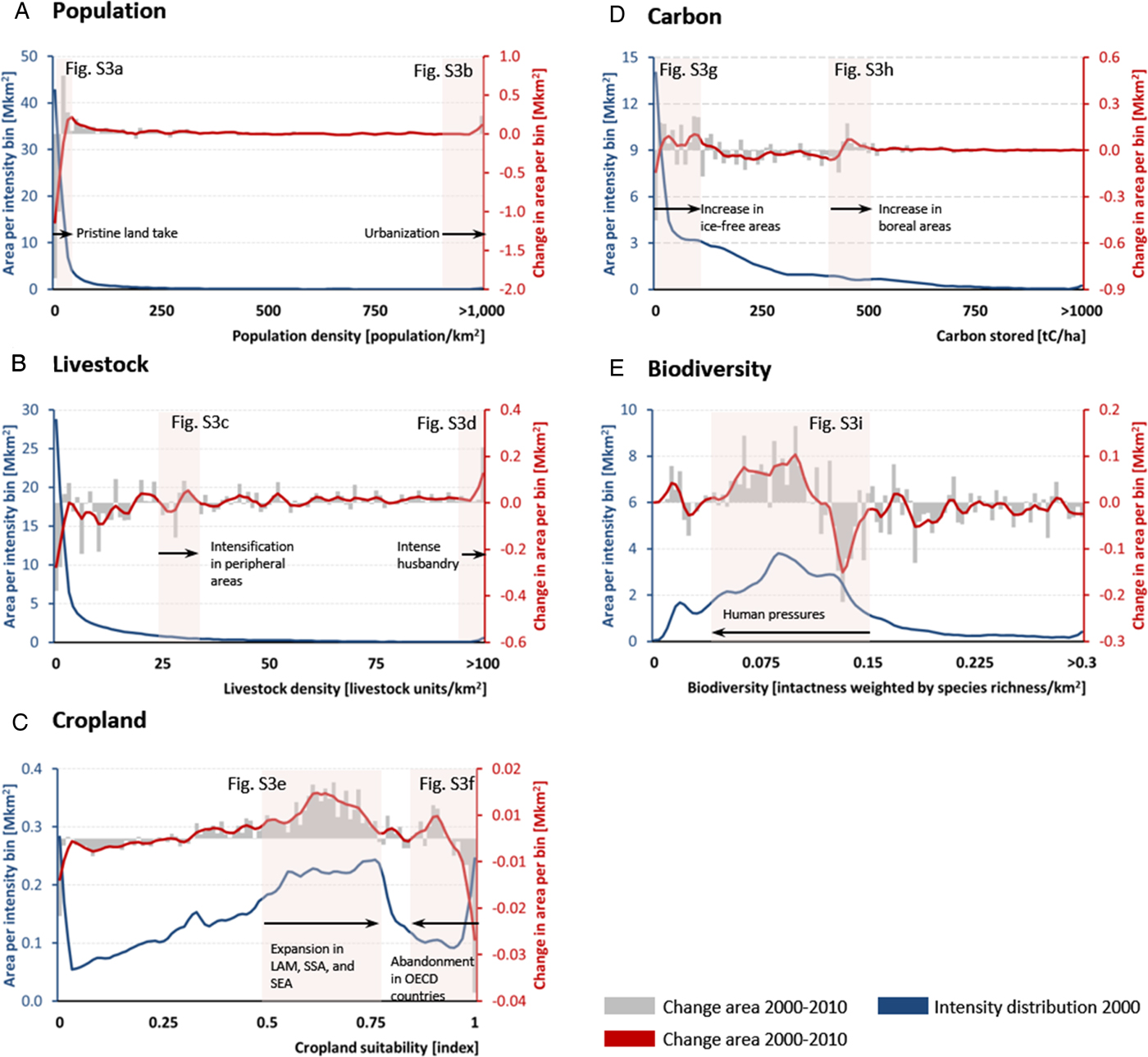
Fig. 2. Distribution of changes in the density of land use between 2000 and 2010 for population (A), livestock (B), cropland (C), carbon (D), and biodiversity (E). Bin sizes are 0.01. Lines represent five-bin weighted mean average. The blue lines represent frequency of land (total area) within each bin; the red lines changes in frequency. Red boxes indicate density bins of special interest and are substantiated with maps in Figure S3 in the Supplementary Information for analysis of spatial patterns, and by the world-region specific review (Tables 2 & 3, & Tables S4 & S5 in the Supplementary Information).
Table 3. Land-use change dynamics in world regions 2000–2010. Key observations were verified by systematic literature review for each world region. See methods for search query, systematic review results in Supplementary Information text, and key references for each world region in Table S7.
3.3. Identifying co-occurrence in land-use changes
Next, we analyzed the spatial co-occurrence of land-use changes by aggregating the area of grid cells on which land-use changes co-occur (Figure 3A). We found that human activities (population, livestock, cropland) tend to grow together, as confirmed by PCA. The first PCA eigenvector, explaining the largest share of data variation, clearly distinguishes between increasing human direct pressures and negative impact on biophysical dimensions (Figure 1F, Figure S1, Figure S2 & Table S2). The second eigenvector describes that increases in population density and terrestrial carbon tend to co-occur with losses in cropland area, biodiversity and, to a lower extent, livestock. This reflects on the one hand cropland and biodiversity reduction due to urban expansion (Bren d'Amour et al., Reference Bren d'Amour, Reitsma, Baiocchi, Barthel, Güneralp, Erb, Haberl, Creutzig and Seto2017) and population growth (India), and on the other hand increased carbon stocks in Europe, the US and in remote areas of the boreal and tropical biomes due to reduced agricultural activity (US, Europe) and CO2 fertilization, respectively.
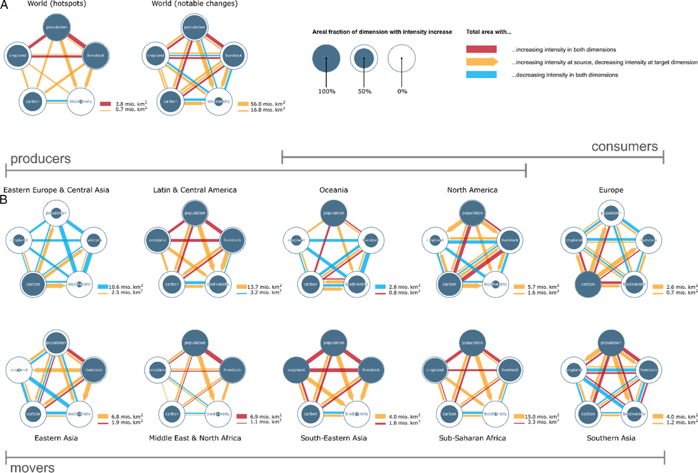
Fig. 3. Co-occurrences of land-use changes between 2000 and 2010 (population, cropland, carbon, biodiversity) and 2000 and 2005 (livestock), respectively, within grid cells for (A) world (hotspots and notable changes), and (B) world regions (notable changes). Solid circle filling represents the area that experienced density increases or decreases within each type of land use. Links between types of land use depict pair-wise co-occurrences. Undirected red (blue) links represent mutual increase (decrease) in density. Reported are gross changes. For example, in some parts of the world, both cropland and livestock decrease simultaneously. In others, they increase simultaneously. This results in both red and blue lines between cropland and livestock. Directed yellow links represent a density increase in source land use, and decrease in target land use. Co-occurrences measured at 0.5° grid resolution. Width of the links shows the respective total area of pair-wise co-occurrence. Links smaller than 2% of total co-occurrence area were omitted.
Biodiversity reduction co-occurs pervasively with density increases for all other land uses (Figure 3A); an observation that is partially a result of the modelling underlying the biodiversity loss data. The highest co-occurrent decrease in land use appears between biodiversity and land carbon stock (Figure 3A). There is an increase in land carbon stock in other areas most likely related to CO2 fertilization, longer growing periods or increased precipitation. In the aggregate perspective of our co-occurrence analysis, in hotspots, population and livestock increase, but carbon stock and especially biodiversity is reduced (Figure 3A). Population exerts a dominant pressure over all land-use changes (Figure 3A). Increases in population where densities are high (urbanization) lead to cropland losses measurable on a global scale. In other locations, cropland expansion coincides with biodiversity loss.
4. Literature review to validate results
4.1. Archetypes of world regions
A world-region specific analysis of co-occurring land-use changes (Figure 3B), substantiated by literature review (Table 3 & Supplementary Information for detailed discussion) and an analysis of the increasingly important role of international trade (Table S3) reveals that regions can be associated with at least one of three types of land-use dynamics (Figure 4). Archetype A is characterized by a large land footprint – but at most moderate population growth (we denote this type as ‘consumers’). Europe fits best into this archetype, with stagnating population, intensification of agriculture and increased reliance on imported foods. Europe outsourced land-intensive food production at a scale corresponding to up-to-half of its domestic cropland use (Figure 4 & Table S3). This enabled a partial recovery of terrestrial carbon and biodiversity. North America and Oceania have high footprints as well, but also feature moderate population growth and high biocapacity enabling exports of its agricultural surplus. Human pressure and losses of ecosystem services have decoupled in only a few instances: land carbon stock and biodiversity are partially co-improving in Europe and Oceania. A possible explanation for the improvement in Europe and Oceania is the emergence of new institutions and policies as, for example, in European Union accession countries from Eastern Europe.
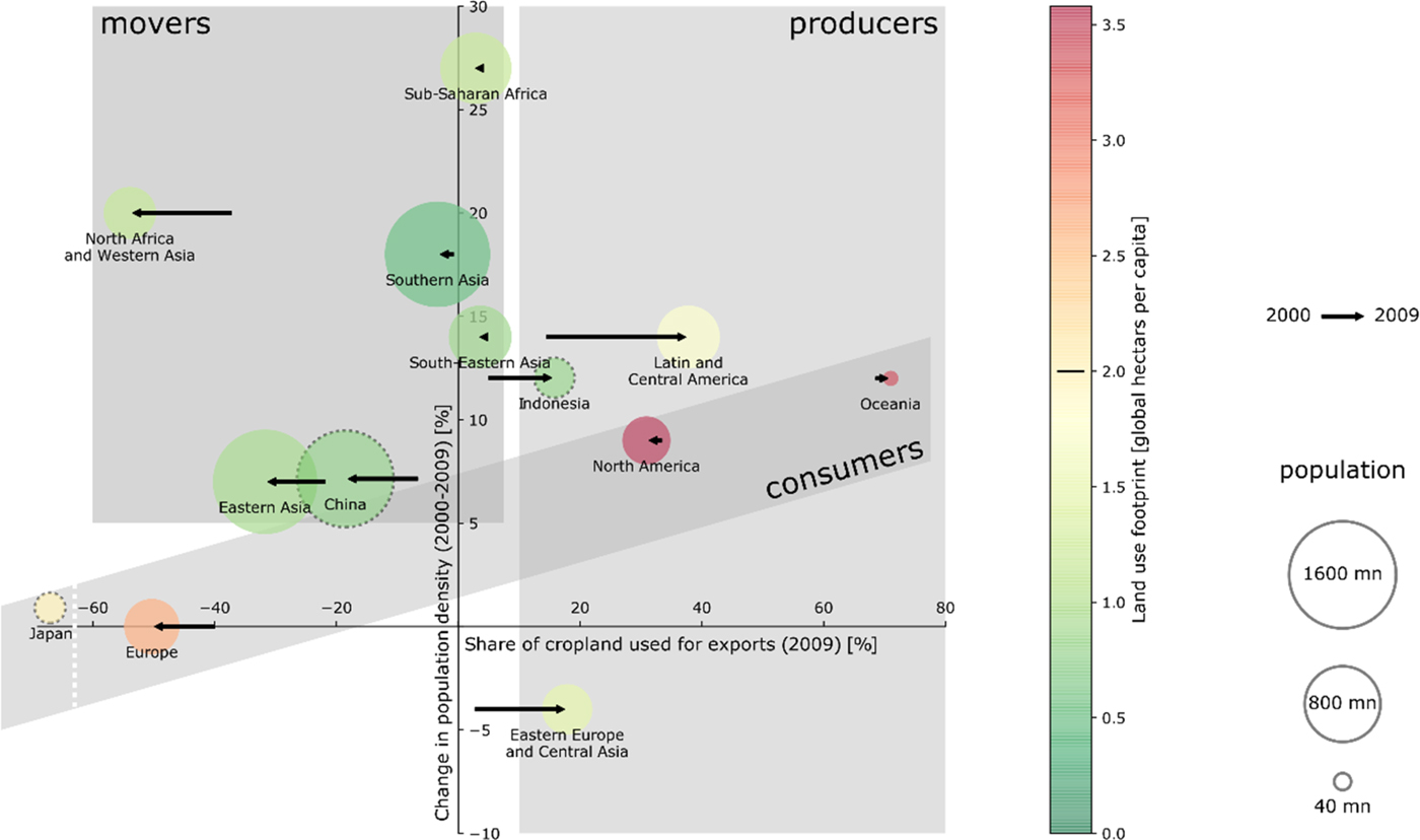
Fig. 4. Land-use change across world regions belongs to different archetypes. Type A (consumers): High land footprint, moderate population growth (Europe, North America, Oceania). Type B (producers): High biocapacity and institutional capacity that enables a share of cropland >10% being exported (Eastern Europe and Central Asia, Latin America, North America, Oceania, South East Asia). Type C (movers): population growth >5% and export share <5%: (North Africa and Western Asia, Southern Asia, Eastern Asia, Sub-Saharan Africa, South Eastern Asia). Data from Kastner et al. (Reference Kastner, Erb and Haberl2014) and Weinzettel et al. (Reference Weinzettel, Hertwich, Peters, Steen-Olsen and Galli2013), see also Table S6 for more detail.
Archetype B is defined by significant export shares (>10% of land is used for export) as enabled by high capacity relative to overall population (‘producers’). Notably, this involves Latin America that increasingly serves the consumer needs of Europe and Eastern Asia. Specifically, South America and Russia increased their cropland embedded in net exports by 24 and 16 percentage points, respectively (Table S3). Importantly, telecoupled and trade-induced land-use links drive biodiversity and carbon loss, epitomized by Latin America, notably in parts of Brazil and the Argentinian Chaco region (Table 3 & Table S3). Also, export of palm oil from Indonesia is a major driver for biodiversity loss and deforestation in South East Asia (Table 3 & Table S3). Overall, exports are responsible for 17% of species loss, with the highest impact embodied in exports from Indonesia to the US and China (Chaudhary & Kastner, Reference Chaudhary and Kastner2016). These insights correspond to the high co-occurrence of decreasing biodiversity and land carbon stock observed in Figure 3A (world) and Figure 3B (especially Latin America, South East Asia). Also, Eastern Europe and Central Asia, witnessing decreasing population, see an increasing share of land used for exports. The consumer world regions of North America and Oceania belong simultaneously to the producers, exporting high margins to other world regions.
Archetype C is characterized by high population growth (>5%) (hence labelled ‘movers’) and limited land used for export (export share of land <5% and increased imports in 2009 compared to 2000). We denote this type as ‘movers’ reflecting their dynamic population and economic growth, and their expected future global influence on global land-use change. Land-use change is dominated by direct regional demands, feeding a growing and more affluent population. A total of 83% of species loss is attributed to agriculture devoted to domestic consumption (Chaudhary & Kastner, Reference Chaudhary and Kastner2016), and demand is increasingly driven by growing affluence and dietary change rather than population growth (Kastner et al., Reference Kastner, Rivas, Koch and Nonhebel2012). Most of Asia and Africa belongs to this archetype. But the variety of ‘mover’ world regions is considerable, ranging from a concurrent expansion of population, livestock and croplands in Sub-Saharan Africa at the cost of natural habitats to strong pressure on cropland by urbanization in Eastern Asia (Figure 3). In fact, a detailed companion study finds that urbanization consumes around 2–3% of global agricultural land between 2000 and 2030, mostly in East Asia; this is prime agricultural land and is nearly twice as productive as average agricultural land, implying a productivity loss of 4–5% (Bren d'Amour et al., Reference Bren d'Amour, Reitsma, Baiocchi, Barthel, Güneralp, Erb, Haberl, Creutzig and Seto2017). Eastern Asia, the Middle East and North Africa import a high proportion of land-based products from elsewhere, similar to Europe. The Middle East and North Africa (MENA) are in the most precarious situation with high population growth and strong reliance on imported food and other land produce (Figure 4).
4.2. Drivers of land-use changes
Here, we report the insights of the systematic literature review on drivers of land-use change helping to interpret the data-based archetypes of world regions and explaining the data-based observations in Table 3. For detailed world-region specific evidence, we refer to Table S7 of the Supplementary Information, and the Supplementary Information text. We identify four robust underlying drivers of land-use changes throughout all regions and strands of literature: population growth and urbanization, institutional drivers, international trade and climate change.
4.3. Population growth and urbanization
Population growth and urbanization is a key driver of land-use changes in many world regions. Population growth and urbanization is closely related to economic growth (Seto et al., Reference Seto, Fragkias, Güneralp and Reilly2011), and the separation of demographic and economic drivers of land-use change is an important question for further research. In East Asia, rapid urbanization and population growth around big metropolitan and urban centres between 2000 and 2010 squeezed other land-use types, for example, by consuming productive croplands (Chen, Reference Chen2007; Galli et al., Reference Galli, Halle and Grunewald2015; Bren d'Amour et al., Reference Bren d'Amour, Reitsma, Baiocchi, Barthel, Güneralp, Erb, Haberl, Creutzig and Seto2017). In India, urban land expansion reduced the harvested area of rice by 4% – but yields increased by 15% (Supplementary Information). In South East Asia, growth in population in cities (>31%) as well as urban land (22%) is high, and dominated by Malaysia, Vietnam, Cambodia, the Philippines and Laos (Schneider et al., Reference Schneider, Mertes, Tatem, Tan, Sulla-Menashe, Graves, Patel, Horton, Gaughan, Rollo, Schelly, Stevens and Dastur2015). The expansion of urban areas and intensification of agriculture has led to cropland loss in the US (Sleeter et al., Reference Sleeter, Sohl, Loveland, Auch, Acevedo, Drummond, Sayler and Stehman2013). However, in other parts of the Americas, especially in parts of the Caribbean and Central America, rural inhabitants abandoned land and migrated to cities, enabling ecosystem recovery (Grau & Aide, Reference Grau and Aide2008). In MENA, human and economic activities congregate around the available, but scarce water resources, such as rivers, oases, or deltas. As a result, human activities compete fiercely for land: by the Nile river in Egypt, urban area expansion is forecast to engulf more than a quarter of valuable croplands (Bren d'Amour et al., Reference Bren d'Amour, Reitsma, Baiocchi, Barthel, Güneralp, Erb, Haberl, Creutzig and Seto2017). Pristine land take in the Arabian Peninsula is closely related to population growth, and agricultural expansion, fostered by unsustainable reliance on fossil water reserves (Odhiambo, Reference Odhiambo2016). In SSA, population dynamics are characterized by high fertility rates and rural–urban migration (Buhaug & Urdal, Reference Buhaug and Urdal2013), driven by population growth in resource constrained rural areas rather than urban agglomeration pull (Holden & Otsuka, Reference Holden and Otsuka2014). Local cropland losses in South Africa coincides with expansion of horticulture (Liebenberg & Pardey, Reference Liebenberg and Pardey2010).
Urbanization has also been an important driver of biodiversity losses. For example, in the Pearl River delta, 26% of natural habitat and 42% of local wetlands have been prey to increasing urban land (He et al., Reference He, Liu, Tian and Ma2014). In India, urbanization also emerged as a key pressure affecting biodiversity loss, but conservation programs and a switch away from traditional fuels ameliorated the loss of biodiversity (Nagendra et al., Reference Nagendra, Sudhira, Katti, Schewenius, Elmqvist, Fragkias, Goodness, Güneralp, Marcotullio, McDonald, Parnell, Schewenius, Sendstad, Seto and Wilkinson2013; Reddy et al., Reference Reddy, Jha, Dadhwal, Krishna, Pasha, Satish, Dutta, Saranya, Rakesh, Rajashekar and Diwakar2015). In Turkey, biodiversity loss appears where important wetlands, grasslands and even rivers are disappearing due to human activities (Şekercioğlu et al., Reference Şekercioğlu, Anderson, Akçay, Bilgin, Can, Semiz, Tavşanoğlu, Yokeş, Soyumert and Ipekdal2011).
The co-occurring population and crop yield growth in the Guinean Savannah is in line with existing evidence on Boserupian intensification in Sub-Sahara Africa (Jayne et al., Reference Jayne, Chamberlin and Headey2014). Cropland expansion, however, also results in a reduction in land carbon stock (cf. Searchinger et al., Reference Searchinger, Estes, Thornton, Beringer, Notenbaert, Rubenstein, Heimlich, Licker and Herrero2015) and land-use emissions for savannah burning exceed those of fossil fuels in Sub-Saharan Africa (Ciais et al., Reference Ciais, Bombelli, Williams, Piao, Chave, Ryan, Henry, Brender and Valentini2011). By contrast, carbon fertilization and increased precipitation generated an increase in land carbon stock in forest areas (Ciais et al., Reference Ciais, Bombelli, Williams, Piao, Chave, Ryan, Henry, Brender and Valentini2011).
4.4. The role of institutions
Analysis of drivers from the literature reveals the importance of institutional drivers, including agricultural policies in Europe and North America, afforestation programs in China, conservation programs in India, forest protection in the Amazon and the legal underpinnings of international trade (see subsequent section).
Land-use change does not inevitably result from population growth and economic dynamics. Instead, institutions and governance usually make the difference. In Europe, changes in the European Common Agricultural Policy explain location-specific reductions in agricultural land use (van Vliet et al., Reference van Vliet, de Groot, Rietveld and Verburg2015).
Energy policy, and specifically biofuel mandates, became a novel driver of land-use change in the 2000s. Biofuel production was responsible for about half the global cropland expansion of about 44Mha between 2000 and 2010; it increased more than four-fold between 2000 and 2010 and, by 2010, biofuels required about 30Mha of land (Bruinsma, Reference Bruinsma2009; Lambin & Meyfroidt, Reference Lambin and Meyfroidt2011). This expansion has mostly taken place on pasture land in Brazil (Lapola et al., Reference Lapola, Martinelli, Peres, Ometto, Ferreira, Nobre, Aguiar, Bustamante, Cardoso, Costa, Joly, Leite, Moutinho, Sampaio, Strassburg and Vieira2014) and, in total, >8Mha of palm oil (only partially used as fuel) in Sumatra, Borneo and Malaysia (Koh et al., Reference Koh, Miettinen, Liew and Ghazoul2011). Biofuel mandates also provided new incentives to expand crop production in the US (Wright & Wimberly, Reference Wright and Wimberly2013), correlating with about 2.3Mha biodiversity-rich prairie land loss in the US from 2008–2012 (Lark et al., Reference Lark, Salmon and Gibbs2015). Wide-spread conversion of grasslands, shrublands and wetlands to agricultural uses (mainly corn and soybean (Faber et al., Reference Faber, Rundquist and Male2012; Wallander et al., Reference Wallander, Claassen and Nickerson2011)) reappeared across the country with hotspots of change located in the Corn Belt and the Lake States.
Better monitoring and more rigorous enforcement in Brazil led to declining deforestation rates after 2005 (Nepstad et al., Reference Nepstad, McGrath, Stickler, Alencar, Azevedo, Swette, Bezerra, DiGiano, Shimada, Motta, Armijo, Castello, Brando, Hansen, McGrath-Horn, Carvalho and Hess2014); The Low-Carbon Agriculture Program and other policies simultaneously supported intensified cattle ranching, especially in the Brazilian subtropics, decoupling husbandry from deforestation (Lapola et al., Reference Lapola, Martinelli, Peres, Ometto, Ferreira, Nobre, Aguiar, Bustamante, Cardoso, Costa, Joly, Leite, Moutinho, Sampaio, Strassburg and Vieira2014). However, in some Brazilian states, institutional failures enable further deforestation by soy producers (Celentano et al., Reference Celentano, Rousseau, Muniz, van Deursen Varga, Martinez, Carneiro, Miranda, Barros, Freitas and da Silva Narvaes2017; Silva & Lima, Reference Silva and Lima2017).
Targeted intentional policies leave a visible mark on global carbon maps. A prime example is China's afforestation policy: afforestation and restored grassland on degraded agricultural land in rural areas (e.g. Tibet, Inner Mongolia) increased terrestrial carbon stock (Deng et al., Reference Deng, Liu and Shangguan2014) (even as cropland extensification, e.g. in the Sichuan basin and Heilongjiang, increased emissions from land-use change (Zhang et al., Reference Zhang, Huang, Chuai, Yang, Lai and Tan2015)).
Institutional change can be a highly important driver of land-use change, even when not intended. As a side effect of the Soviet collapse, rural emigrants abandoned farms enabling reforestation (>30Mha) (Kuemmerle et al., Reference Kuemmerle, Levers, Erb, Estel, Jepsen, Müller, Plutzar, Stürck, Verkerk and Verburg2016) in former socialist countries. Land-use change varied however between former socialist countries, which has been attributed to strong differences in market reform (Alcantara et al., Reference Alcantara, Kuemmerle, Baumann, Bragina, Griffiths, Hostert, Knorn, Müller, Prishchepov and Schierhorn2013). In European Russia the gain amounts to more than 44tCO2/ha during our observation period, which makes it outstanding as a sink in the boreal region and comparable to sinks in the temperate biome (Pan et al., Reference Pan, Birdsey, Fang, Houghton, Kauppi, Kurz, Phillips, Shvidenko, Lewis, Canadell, Ciais, Jackson, Pacala, McGuire, Piao, Rautiainen, Sitch and Hayes2011). Varied patterns exist in carbon stock changes, partially depending on the timing of land abandonment (Schierhorn et al., Reference Schierhorn, Müller, Beringer, Prishchepov, Kuemmerle and Balmann2013).
4.5. International trade
As a specific institutional driver, emerging literature increasingly emphasizes globalized markets for land-use changes, which dramatically shifts the interpretation of regionally observed land-use changes. As a prime case, Europe outsources land-intensive crop production through international trade: the share of ‘imported’ cropland, driven by dietary change (Galli et al., Reference Galli, Iha, Halle, El Bilali, Grunewald, Eaton, Capone, Debs and Bottalico2017), grew by 20% from 2000 to 2009 and by then corresponded to more than half of the cropland under domestic production (Table S3). Both agricultural intensification of the most productive lands (e.g. in Denmark) and farmland abandonment in marginal, less competitive regions are driven by the globalization of agricultural markets (van Vliet et al., Reference van Vliet, de Groot, Rietveld and Verburg2015; Kuemmerle et al., Reference Kuemmerle, Levers, Erb, Estel, Jepsen, Müller, Plutzar, Stürck, Verkerk and Verburg2016).
The MENA region is also found to outsource land-intensive production by imports, which have increased substantially between 2000 and 2010 (Galli et al., Reference Galli, Iha, Halle, El Bilali, Grunewald, Eaton, Capone, Debs and Bottalico2017) (Table S3), increasing the risk for telecoupled food supply shocks (Bren d'Amour et al., Reference Bren d'Amour, Wenz, Kalkuhl, Steckel and Creutzig2016). A major driver is large population growth; in Morocco, for example, food demand multiplied driven by population growth (160% in 1961–2009) and per capita demand (>50% in 1961–2009) (Galli, Reference Galli2015).
Economic growth in East Asia resulted in telecoupled land-use changes. For example, Chinese demand for timber has driven deforestation and hence carbon-loss in South East Siberia (Liang et al., Reference Liang, Guo, Newell, Qu, Feng, Chiu and Xu2016). While meat demand resulting from increasing incomes and economic growth in East Asia (Thornton, Reference Thornton2010) is mostly satisfied by industrialized livestock breeding, particularly in urban areas (Bai et al., Reference Bai, Ma, Qin, Chen, Oenema and Zhang2014), increasing fodder imports to East Asia, particularly maize and soybean, for livestock production have raised land-use pressures elsewhere (particularly in Latin America and South East Asia) as the proportion of indirect cropland imports grew (Table S3).
Land-use change for exported goods is pervasive in tropical regions. In Latin America, farmers and companies increasingly produced and exported soy and maize for markets in Europe and East Asia (Kastner et al., Reference Kastner, Erb and Haberl2014), driven by a combination of the availability of fertile land and low production costs, especially in the peripheral Amazon basin (Grau & Aide, Reference Grau and Aide2008) and the Argentinian Chaco region (Gasparri & Grau, Reference Gasparri and Grau2009) (Figure 1). In South East Asia palm oil production drives deforestation (Hosonuma et al., Reference Hosonuma, Herold, De Sy, De Fries, Brockhaus, Verchot, Angelsen and Romijn2012) (>30% for international markets (Wilcove et al., Reference Wilcove, Giam, Edwards, Fisher and Koh2013)). In addition, it is sometimes related to large-scale land acquisitions (Davis et al., Reference Davis, Yu, Rulli, Pichdara and D'Odorico2015) and causes severe losses of biodiversity in South East Asia. The draining and burning of peatland releases large amounts of carbon, especially in Sumatra, and to a lesser degree in Borneo (Wilcove et al., Reference Wilcove, Giam, Edwards, Fisher and Koh2013). To understand the scale: in 2015, peak emissions from deforestation and fires in South East Asia exceeded those of the European Union fossil fuel burning (Huijnen et al., Reference Huijnen, Wooster, Kaiser, Gaveau, Flemming, Parrington, Inness, Murdiyarso, Main and van Weele2016).
In Sub-Saharan Africa cropland dynamics have largely been driven by local factors rather than by international trade (Table S3). Rural densification and biodiversity loss is most strongly associated with population pressure, but also with cropland expansion (Searchinger et al., Reference Searchinger, Estes, Thornton, Beringer, Notenbaert, Rubenstein, Heimlich, Licker and Herrero2015). Lack of infrastructure and low investment rates resulting from poor institutional quality have thus far impeded a further integration of SSA in international agricultural markets (Barrett, Reference Barrett2008; Kalkuhl, Reference Kalkuhl2016)
4.6. Anthropogenic climate change
Region-specific dynamics demonstrate that anthropogenic climate change already affects land-use change. Carbon fertilization has especially affected carbon stocks in the intact tropical rainforests, such as in Congo, and the boreal zone, including Siberia (Zhu et al., Reference Zhu, Piao, Myneni, Huang, Zeng, Canadell, Ciais, Sitch, Friedlingstein, Arneth, Cao, Cheng, Kato, Koven, Li, Lian, Liu, Liu, Mao, Pan, Peng, Peñuelas, Poulter, Pugh, Stocker, Viovy, Wang, Wang, Xiao, Yang, Zaehle and Zeng2016). Increased precipitation in the Sahel zone (Park et al., Reference Park, Bader and Matei2016) and Central Africa enabled higher carbon stocks, while salinization and droughts, partially attributed to anthropogenic climate change (Gallant et al., Reference Gallant, Kiem, Verdon-Kidd, Stone and Karoly2012), compromised more than half of the farmland and crop production in Australia (MSEIC, 2010) (see also Table S5).
5. Discussion and conclusion: towards managing global land-use change
In this paper, we investigated data on global land use between 2000 and 2010, and reviewed the corresponding land-use change. We fill an important gap as other literature is either focused on one land-use dimension, such as food (Bruinsma, Reference Bruinsma2009) or biodiversity (Newbold et al., Reference Newbold, Hudson, Hill, Contu, Lysenko, Senior, Börger, Bennett, Choimes and Collen2015), or investigates century-long time scales (Hurtt et al., Reference Hurtt, Chini, Frolking, Betts, Feddema, Fischer, Fisk, Hibbard, Houghton and Janetos2011). We find that human-related activities – population growth, and agricultural and livestock intensification – co-occur on coarse spatial scales, and that biodiversity is under pressure worldwide. Our data and literature-based assessment also reveals that the regionally diverging patterns of global land-use change are grounded in direct human pressures, domestic institutions, telecoupled land demand by international trade and varying climate change impacts. We identify three archetypes of world regions: (A) ‘consumers’, characterized by high per capita land footprint, such as Europe; (B) ‘producers’, characterized by a significant export share of land, such as Latin America; and (C) ‘movers’, characterized by high population growth and increasing demand for land outside their own regions, such as South Asia. Due to its population and dynamic change, the ‘movers’ will have the most important role in future global land-use change. These results are useful for global assessments of land-use change and are a baseline for further research. Our data comparison ends in 2010, but more recent dynamics further underline the importance of continuously capturing the human-related activities across scales as the example of deforestation shows: in the period from 2010–2015, tropical forest continued to decrease by 5.5Mha/year, while temperate forest increased by 2.2Mha/year (Keenan et al., Reference Keenan, Reams, Achard, de Freitas, Grainger and Lindquist2015).
The results also provide motivation and orientation for governing global land use. We complement other scientific findings (e.g. Lepers et al., Reference Lepers, Lambin, Janetos, DeFries, Achard, Ramankutty and Scholes2005; Lambin & Geist, Reference Lambin and Geist2008) in providing further evidence and spatial information on the force and direction of anthropogenic land-use change. Both the global importance of biodiversity and food security, and the telecoupled nature of land-use change drivers point to the importance of international coordination to manage global land use. Managing global land-use change requires an explicit consideration of the socio-economic, biophysical and institutional differences between world regions. The strong telecoupling, both by international trade and climate change, substantiate the need for international cooperation to manage global land (Magalhães et al., Reference Magalhães, Steffen, Bosselmann, Aragão and Soromenho-Marques2016; Creutzig, Reference Creutzig2017), supporting national and local policies. In consumer regions, such as Europe, sustainability certificates and dietary change could foster a shift to sustainable land use on the demand side (Tayleur et al., Reference Tayleur, Balmford, Buchanan, Butchart, Ducharme, Green, Milder, Sanderson, Thomas, Vickery and Phalan2016; Galli et al., Reference Galli, Iha, Halle, El Bilali, Grunewald, Eaton, Capone, Debs and Bottalico2017). In producer regions, in particular those with rich biodiversity, harmonization of ecosystem protection measures and financing of nature conversation (le Polain de Waroux et al., Reference le Polain de Waroux, Garrett, Heilmayr and Lambin2016), and an upscaling of international payment for ecosystem services schemes (Rands et al., Reference Rands, Adams, Bennun, Butchart, Clements, Coomes, Entwistle, Hodge, Kapos, Scharlemann, Sutherland and Vira2010) would be a key component of protecting intact ecosystems. As carbon stock movements are not always related to biodiversity, it is crucial for the design of environmental policies to differentiate between land carbon stocks and biodiversity (Phelps et al., Reference Phelps, Webb and Adams2012). Complementing payments for ecosystems, land taxes are discussed as a new policy instrument that would reduce pressure on ecosystems (Kalkuhl, & Edenhofer, Reference Kalkuhl and Edenhofer2017; Kalkuhl et al., Reference Kalkuhl, Milan, Schwerhoff, Jakob, Hahnen and Creutzig2018; Tahvonen & Rautiainen, Reference Tahvonen and Rautiainen2017). Our data reveals that in Sub-Saharan Africa and Latin America rural population growth is accompanied by an increase in cropland and a reduction in biodiversity (Figures 1 & 3), pointing to potential expansions in agricultural production due to population pressure (cf. Boserup, Reference Boserup2005). Specific measures to further improve efficient land use involve intensification that complies with the protection of important ecosystems, soil carbon and water resources (Garnett et al., Reference Garnett, Appleby, Balmford, Bateman, Benton, Bloomer, Burlingame, Dawkins, Dolan, Fraser, Herrero, Hoffmann, Smith, Thornton, Toulmin, Vermeulen and Godfray2013); multi-purpose systems that integrate several land uses, an approach called land sharing (Lambin & Meyfroidt, Reference Lambin and Meyfroidt2011; Fischer et al., Reference Fischer, Abson, Butsic, Chappell, Ekroos, Hanspach, Kuemmerle, Smith and von Wehrden2014); and compact urbanization that preserves cropland (Bren d'Amour et al., Reference Bren d'Amour, Reitsma, Baiocchi, Barthel, Güneralp, Erb, Haberl, Creutzig and Seto2017). Improved land tenure and property rights can facilitate adoption of sustainable land-use management with positive impacts on carbon stocks and biodiversity (Abdulai et al., Reference Abdulai, Owusu and Goetz2011; Abdulai & Goetz, Reference Abdulai and Goetz2014; Robinson et al., Reference Robinson, Holland and Naughton-Treves2014a; Etongo et al., Reference Etongo, Djenontin, Kanninen, Fobissie, Korhonen-Kurki and Djoudi2015). Prioritizing a small set of leverage points could greatly increase the sustainability and efficiency of food production (West et al., Reference West, Gerber, Engstrom, Mueller, Brauman, Carlson, Cassidy, Johnston, MacDonald, Ray and Siebert2014).
Improving institutional capacity emerges as a key factor for realizing nature conservation and efficient land use. It will be an important task of further research to identify the most effective options for both local action and international cooperation to sustainably manage global land-use change.
Supplementary material
The supplementary material for this article can be found at https://doi.org/10.1017/sus.2018.15
Author ORCIDs
Felix Creutzig 0000-0002-5710-3348
Acknowledgements
The authors thank Global Forest Watch for sharing data and Tim Newbold for help with interpreting data. The authors also thank Jan Minx and Annika Marxen for support in early stages of this project.
Author contributions
F. C. designed the project with inputs from all authors. C. B. D. A., U. W., T. B., A. G., A. R., M. K. and F. C. performed data analysis. All authors contributed to reviewing the literature and writing.
Financial support
None.
Conflict of interest
None.
Ethical standards
This research and article complies with Global Sustainability's publishing ethics guidelines.


 Open access