Introduction

During the last two decades many global climate models (GCMs) have been used to simulate the climate of the Last Glacial Maximum (LGM). In the last 5–10 years, however, all of the major boundary conditions that are prescribed for these simulations have been questioned or revised. The timing of the LGM as defined by δ¹⁸O deep-sea-core records has been revised from 21000 to 18 000 years ago (Reference Bard, Hamelin, Fairbanks and ZindlerBard and others, 1990), thus changing the orbital elements with small, but perceptible, effects on climate simulations (Reference Hyde and PeltierHyde and Peltier, 1993). The CLIMAP (1981) ice-sheet reconstructions used until recently by most GCM simulations are being superceded by the more sophisticated reconstructions of Reference PeltierPeltier (1994), whose ICE-4G Laurentide and Eurasian ice sheets are much thinner than those of CLIMAP. And since the mid-1980s, data have accumulated that question the relatively small 1–2°C cooling of tropical and subtropical seasurface temperatures estimated by the planktonic transferfunction techniques of CLIMAP (1981). This includes independent evidence of greater cooling on low-latitude land masses (e.g. Reference Rind and PeteetRind and Peteet, 1985) and at least one tropical sea-surface temperature (SST) site (Reference Guilderson, Fairbanks and RubenstoneGuilderson and others, 1994), suggesting cooling of ∼5°C. The effects of these different SSTs and ice-sheet boundary conditions on LGM climate simulations are potentially significant, and are just beginning to be explored.

One fact concerning the LGM has not changed: about 21000 years ago (henceforth 21 ka BP) the global ice volume as measured by deep-sea-core δ¹⁸O records reached a maximum value. This was preceded by at least 5000 years of strong positive global-ice growth, and succeeded by about 15 000 years of overall rapid ice-melt during the last deglaciation (e.g. Reference Imbrie, Berger, Imbrie, Hays, Kukla and SaltzmanImbrie and others, 1984; Reference ShackletonShackleton, 1987). This is roughly consistent with terrestrial geologic records left by the Laurentide and Eurasian ice sheets, the southern margins of which, by and large, reached their maximum extents around that time (Denton and Hughes, 1981; Reference Dyke and PrestDyke and Prest, 1987; Reference RuddimanRuddiman and Wright, 1987; Reference ClarkClark, 1994). The straightforward implication is that the net annual mass balance of ice sheets and glaciers worldwide was positive from at least 25–21 ka BP, nearly zero for a period around 21 ka BP, and became strongly negative shortly after 21 ka BP.

In principle this provides a test of GCMs and the prescribed boundary conditions used to simulate the LGM climate. In those GCMs where the surface mass balance over all ice-sheet points is calculated, the global surface icesheet mass budget can be predicted. According to the above rationale, this value should be relatively small, or positive to balance basal melt and iceberg/ice-shelf discharge, but should not be strongly negative. If it were strongly negative, it would suggest either that the GCM physics is wrong, or that one or more of the boundary conditions used in the simulation (prescribed SSTs, prescribed ice-sheet extent and elevations, or atmospheric CO₂ amount) are in error, and are producing too much melt and/or too little precipitation on the ice sheets. By “strongly negative”, we mean values that would correspond to a global eustatic sea-level rise of ∼1 cm a^–1 or more (a typical rate during the last deglaciation), or a complete wastage of individual ice sheets in less than ∼10 000 years.

In order for this test to be meaningful, the GGM physics involved in ice-sheet mass balance should be reasonably realistic, and the results for present-day ice sheets should be close to observed estimates. However, most previous GCM calculations of surface mass budgets for present-day Greenland have been severely in error, mainly due to problems of scale and to the neglect of refreezing of meltwater. As described below, we have recently addressed these problems in a new version of the Global ENvironmental and Ecological Simulation of Interactive Systems (GENESIS) GCM, and have obtained good present-day simulations of the precipitation, ablation and mass balance on Greenland and Antarctica (Reference Thompson and PollardThompson and Pollard, 1997). The main purpose of this paper is to present LGM results using this GCM and various combinations of SSTs (predicted and prescribed) and ice-sheet prescriptions, focusing on the predicted mass balances of the Laurentide and Eurasian ice sheets, and to discuss the overall consistency of the results.

The next section outlines the formulation of the GENESIS GCM, and defines the experimental setup and boundary conditions used for the LGM simulations. The third section outlines the methods used to predict ice-sheet budgets in this GCM, and presents these budgets for various LGM simulations with predicted and prescribed SSTs and different ice-sheet reconstructions. It is found that, for all plausible combinations of boundary conditions, the predicted ice-sheet budgets appear to be too negative. Some of the consequences of this are discussed in the final section, including speculation on ice-sheet evolution in the several thousand years leading up to the LGM.

Global Climate Model Description

The GCM used here is version 2.0. a of GENESIS (hereafter abbreviated to version 2). It has been developed at NCAR with emphasis on terrestrial, biophysical and cryospheric processes, for the purpose of performing greenhouse and paleoclimatic experiments. An earlier version (1.02) of the model with coarser atmospheric resolution has been described in Reference Thompson and PollardThompson and Pollard (1995a, Reference Thompson and Pollardb) and Reference Pollard and ThompsonPollard and Thompson (1994,Reference Pollard and Thompson1995). Present-day results with version 2 are significantly improved over version 1.02, and the new physics in version 2 and its present-day climate including Greenland and Antarctic mass balance is described in Reference Thompson and PollardThompson and Pollard (1997). More information on the global climate of the 21 ka BP simulations is included in Reference Pollard and ThompsonPollard and Thompson (in press) and a further application coupled to a dynamic ice-sheet model is described in Reference Pollard and ThompsonPollard and Thompson (1997). For brevity, only a few basic features of the model are mentioned here; more complete descriptions are given in the above references.

The standard version-2 model consists of an atmospheric GCM (AGCM) coupled to multi-layer models of vegetation, soil or land ice, and snow. SSTs and sea ice are computed using a 50 m slab oceanic layer. The AGCM grid is independent of the surface grid, and fields are transferred between the AGCM and the surface by bi-linear interpolation (AGCM fields to surface) or straightforward area-averaging (surface fluxes to AGCM) at each time-step. The nominal AGCM resolution is spectral T31 (∼3.75° x 3.75°) with 18 vertical levels, and the surface grid used for all surface models is 2° x 2°, with an overall GCM time-step of 0.5 hours. These resolutions were used for the GCM experiments described below.

A land-surface transfer model (LSX) accounts for the physical effects of vegetation (Reference Pollard and ThompsonPollard and Thompson, 1995). Up to two vegetation layers (“trees” and “grass“) can be specified at each grid point, and the radiative and turbulent fluxes through these layers to the soil or snow surface can be calculated. Vegetation attributes, such as leaf-area indices, fractional cover, leaf albedos, etc., are prescribed from present-day off-line results of a predictive naturalvegetation model (the EVE model; personal communication from J. C. Bergengren, 1996). No modifications to the present-day natural vegetation have been made for the 21 ka BP experiments in this paper.

A 6-layer soil model extends from the surface to 4.25 m depth, with layer thicknesses increasing from 5 cm at the top to 2.5 m at the bottom. Physical processes in the vertical soil column include heat diffusion, liquid-water transport, surface runoff and bottom drainage, uptake of liquid water by plant roots for transpiration, and the freezing and thawing of soil ice. The same 6-layer model is used for ice-sheet surfaces, with physical parameters appropriate for ice, and with internal-liquid moisture. A 3-layer snow model is used for snow cover on soil, ice-sheet and sea-ice surfaces, including fractional areal cover when the snow is thin.

A 3-layer thermodynamic sea-ice model predicts the effect of local melting and freezing on the ice thickness and fractional areal coverage. Sea-ice advection is included using the “cavitating-fluid” model of Reference Flato and HiblerFlato and Hibler (1992), using AGCM surface winds and prescribed ocean currents. The ocean is represented by a 50 m thick thermodynamic slab, which crudely captures the seasonal heat capacity of the surface-mixed layer. Oceanic heat transport is treated as horizontal diffusion down the gradient of the mixed-layer temperature, with the diffusion coefficient depending on latitude to produce roughly the present observed zonal-mean transport. A region of enhanced winter-flux convergence in the Norwegian Sea is specified that keeps the region ice-free, as observed for the present day, and an additive global adjustment is made at each time-step to ensure that the global integral of the convergence is zero.

Ice-Sheet Budgets

The precipitation, melting and evaporation over the model ice sheets at the LGM are determined by the simulated climate, notably by storm tracks, surface-air temperatures, surface winds and cloudiness. These and other global-model fields for 21 ka BP are described in Reference Pollard and ThompsonPollard and Thompson (in press), and compared in some detail with proxy data and results from other GCMs. For brevity, we will not reproduce these global climate results here, but concentrate instead on the mass balance over the ice sheets.

In order to test the GCM's predictions for LGM icesheet mass balance, the model physics involved in those processes must be reasonably realistic. However, there are two significant problems in using GCMs to predict massbalance distributions on ice sheets: (i) the relatively coarse GCM horizontal resolution truncates the topography of the ice-sheet flanks and smaller ice sheets such as Greenland, and to a lesser extent the Eurasian and the flanks of the Laurentide, and (ii) the snow and ice physics in most GCMs does not include ice-sheet-specific processes such as the re-freezing of meltwater.

Due partly to these shortcomings, the simulated budgets of present-day Greenland and/or the LGM Laurentide and Eurasian ice sheets have been much too negative in many earlier coarse- and medium-resolution GCMs (Reference Manabe and BroccoliManabe and Broccoli, 1985; Reference RindRind, 1987; Reference Broccoli, Manabe and PeltierBroccoli and Manabe, 1993). In GENESIS version 2 two techniques are employed that attack these problems (Reference Thompson and PollardThompson and Pollard, 1997). For the scale problem, the AGCM meteorological fields passed to the ice-sheet surface model at each time-step are (i) interpolated to the 2° x 2° surface grid as for all surface models, and (ii) corrected for the error between the AGCM spectrally truncated topography and the true 2° x 2° topography, using simple adjustments based on a constant lapse rate of –7.0°C km^–1. (This value is an estimate of the change in surface-air temperature that would result in a vertical shift of the large-scale surface itself; it has no obvious relationship to the free-air temperature profiles predicted by the GCM above the spectrally truncated surface.) Furthermore, a post-processing correction of the refreezing of meltwater is made to the annual history fields over ice sheets, following Reference Pfeffer, Meier and IllangasekarePfeffer and others (1991); this parameterization reduces the account of local snow and ice-melt that becomes mobile enough to escape the ice sheet, depending on the ratio of the annual melt to the previous winter's snowpack. With these two corrections the model's precipitation, ablation and surface mass balances for present-day Greenland and Antarctica lie well within the mid-ranges of recent observed estimates (Reference Warrick, Oerlemans, Houghton, Jenkins and EphraumsWarrick and Oerlemans, 1990; Reference Van der VeenVan der Veen, 1991; Reference Meier and PeltierMeier, 1993; Reference Warrick, Le Provost, Meier, Oerlemans, Woodworth, Houghton, Meira Filho, Callander, Harris, Kattenberg and MaskellWarrick and others, 1996; Reference Thompson and PollardThompson and Pollard, 1997), so we may expect the same techniques applied to the LGM ice sheets should substantially nullify the above sources of error.

In presenting our results below we use precipitation (snowfall plus rainfall), rather than accumulation, which has various usages in the literature (sometimes including or excluding rainfall, evaporation, and/or wind-blown snow). In addition, we use the term “runoff” to imply that part of the local surface melt and rainfall on bare ice that escapes according to the refreezing parameterization; “ablation” refers to the escaped runoff plus evaporation; and “mass balance” is the net surface budget (precipitation minus ablation). For the areally averaged ice-sheet budgets reported below, we compute averages over the Laurentide and Cordilleran ice sheet separately, taking the view that they remained dynamically distinct through the LGM. Greenland is also reported as a distinct ice sheet, divided from the Laurentide by a line running north-northeast between Ellesmere Island and Greenland, and not including Iceland (Ellesmere Island and the rest of the Canadian Archipelago are considered part of the Laurentide). Budgets for the Eurasian ice sheet do not include the separate ICE-4G British and Siberian ice sheets, and similarly budgets for Antarctica do not include the separate ICE-4G Patagonian (southern Andes) and New Zealand ice sheets. However, the “global” averages below include all ice-sheet surfaces in the model including the minor ice masses.

With ICE-4G ice sheets

Figures 1 and 2 show annual precipitation, ablation and net balance fields at the LGM for the ICE-4G ice sheets, with prescribed SSTs (Fig. 1) and predicted SSTs (Fig. 2). The fields are similar for the two types of simulations, as might be expected from the similarity of the temperature and precipitation changes over land (Reference Pollard and ThompsonPollard and Thompson, in press). For the Laurentide, the largest precipitation of 50- 100 cm a^–1 occurs on the southern flanks. Higher values of 100-200 cm a^–1 occur on the western flank of the Cordilleran ice sheet, presumably due to orographic uplift of the westerlies, and this causes a “shadow” region of reduced precipitation on the western Laurentide. Precipitation rates over the higher Laurentide interior are much lower, ranging from ∼5-30 cm a^–1, There is also very little ablation in most of the interior (Figs lb and 2b). Around the much lower southern flanks, however, several meters of ice melt each year. This is reflected in the net mass balance (Figs lc and 2c), with positive values of up to ∼50 cm a^–1 over most of the interior, and much larger negative values around the southern and western flanks and in the Cordilleran–Laurentide divide.

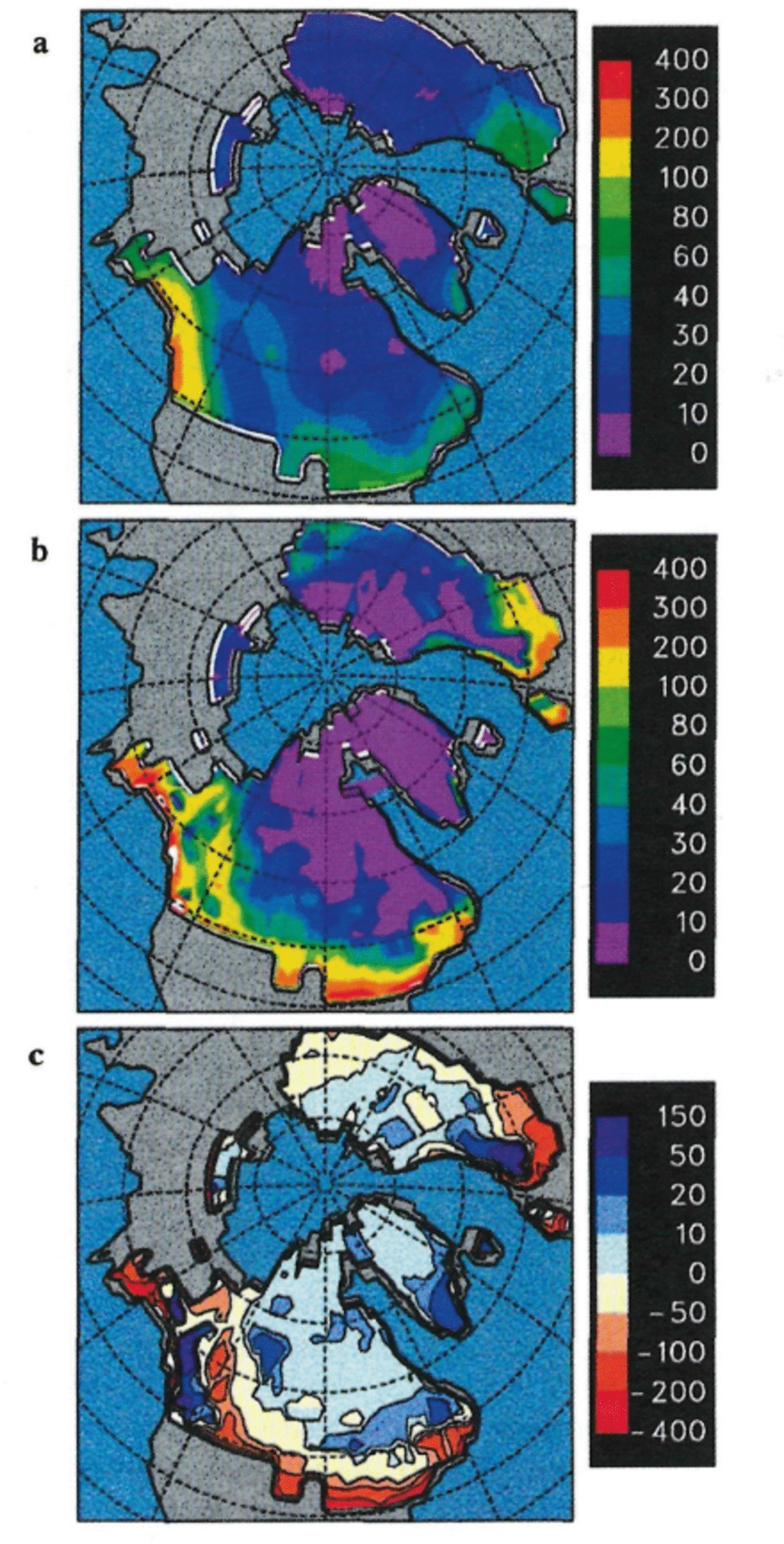
Fig. 1. Ice-sheet surface mass-budget terms over Northern Hemispheric ice sheets for 21ka BP, in cm a , with ICE-4G ice sheets and prescribed SSTs and sea ice. (a) Annual precipitation, (b) Annual ablation (surface melt and rainfall that escapes the ice sheet, plus evaporation), (c) Net annual surface budget (precipitation minus ablation).

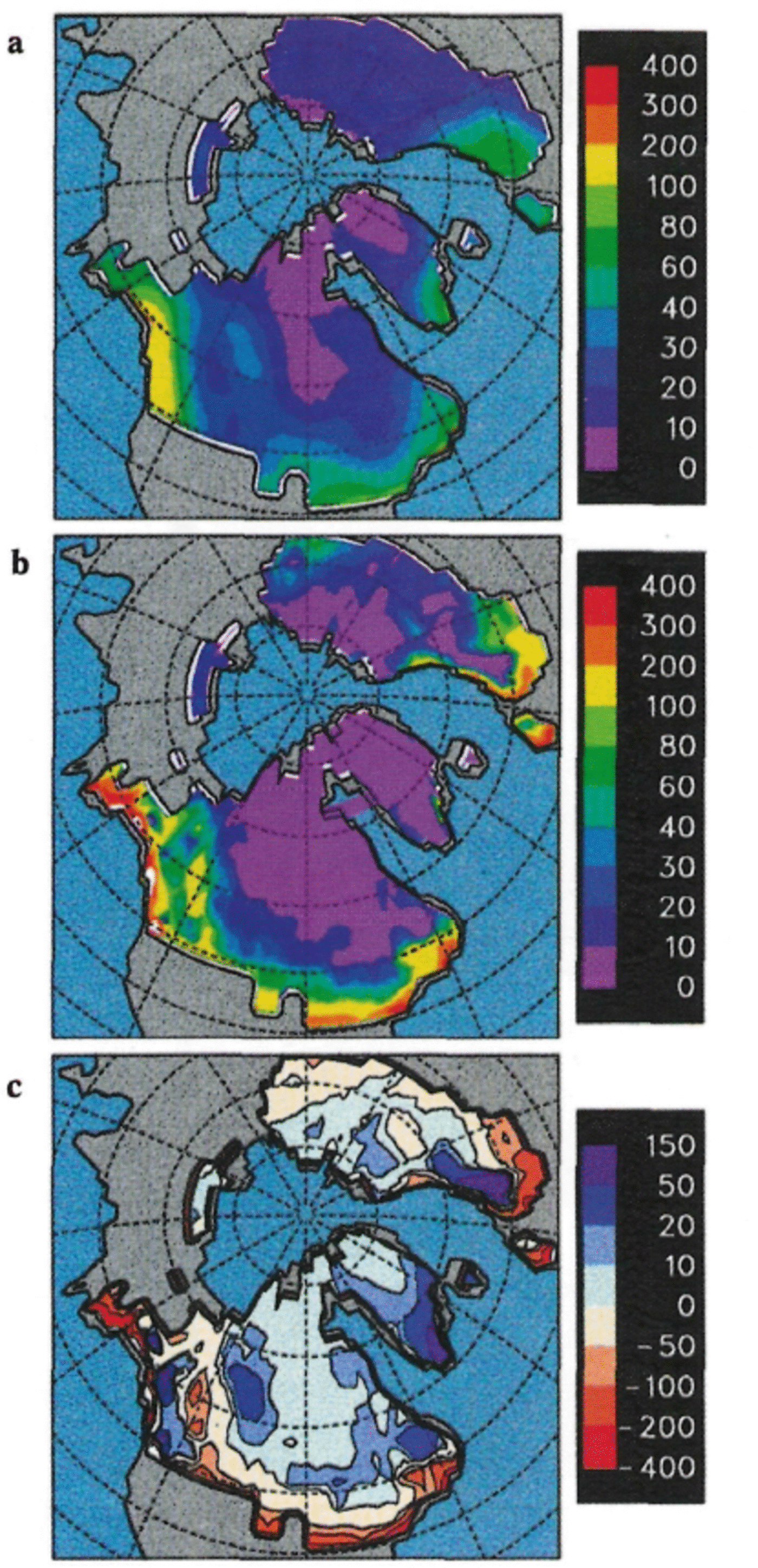
Fig. 2. As Figure 1, except with predicted SSTs and sea ice.

The areal and annual mean surface mass balance for the ICE-4G Laurentide shown in Table 1 is –17 cm a^–1 (predicted SSTs) or –31 cm a^–1 (prescribed SSTs), dominated by the melting around the southern flanks. The prescribed SST budget is more negative because of greater total ablation (not shown), which we suspect is due to warmer subtropical CLIMAP SSTs causing slightly warmer surface-air temperatures over the southern flanks. Dividing these budget values into a rough average thickness of the ice sheet (1600 m), implies time-scales for complete wastage of ∼9400 or 5100 years, respectively. This does not necessarily mean that a hypothetical ice sheet would vanish in exactly that time given our surface forcing; it might do so faster (due to warmer air temperatures as its elevations decrease, and/or due to additional wastage by iceberg/ice-shelf discharge), or only the low southern flanks might vanish leaving a high central core with steeper edges. But in any case, the geologic, δ¹⁸O and sea-level records suggest that the LGM ice sheets, and even the peripheral Laurentide lobes, did not begin such major retreats until shortly after the LGM, so at first sight these overall surface budgets for the LGM Laurentide are much too negative. This will be discussed further in the next section.

Table 1. Ice-sheet annual mean net surface mass balances in cm^-2 a^-1 (or cm a^-1 ojliquid water equivalent), for the present and 21 ka BP, and for various model runs with prescribed and predicted SSIs and different ice-sheet reconstructions. The last row excludes the relatively small British, Siberian, Patagonian, New Zealand and Iceland ice sheets from the global average. Standard deviations due to inter-annual variability (not shown) are mostly 5~10 % of the mean values, so the resultant uncertainties in the multi-year means are relatively small.

The annual surface mass balance for the ICE-4G Cordilleran ice sheet is –131 cm a^–1 (predicted SSTs) or – 117 cm a^–1 (prescribed SSTs). Conceivably some surface loss could have been balanced by ice flow from the Laurentide, since the extent of coalescence of the Laurentide and Cordilleran ice sheets at LGM is not well known (Denton and Hughes, 1981). Even with this caveat, we consider such large negative Cordilleran budgets to be very unrealistic (see below).

The patterns of precipitation, ablation and mass balance on the Eurasian ice sheet at LGM are quite similar to those on the Laurentide (Figs 1 and 2). Relatively large amounts of precipitation fall on the southwestern flanks, presumably due to orographic uplift of the westerlies, and several meters of ice melts each year around the southern and western flanks. The overall annual budget (Table 1) is –16 cm a^–1 (predicted SSTs) or –20 cm a^–1 (prescribed SSTs). Dividing these into a rough average thickness of the ice sheet (900 m), the implied time-scales for complete wastage are ∼5000 years.

Since the δ¹⁸O and eustatic sea-level records represent variations of global ice volume, it is of interest to examine the budgets of the other major ice sheets in the model. For Greenland, the net annual surface budget is 16 cm a^–1 (predicted SSTs) or 9 cm a^–1 (prescribed SSTs), quite close to the model's present-day values of 15 or 18 cm a ^–1 although the LGM precipitation and ablation arc both much reduced in magnitude from the present. The positive Greenland regime, compared to the negative ICE-4G Laurentide and Eurasian values, is due to the more northern location of Greenland, and also to its much steeper flanks and consequently much narrower ablation zones.

The net surface budget for Antarctica at the LGM is 16 cm a ^–1 (predicted SSTs) or 12 cm a ^–1 (prescribed SSTs), compared to the model's present-day values of 20 and 17 cm a^–1. This is due to slightly less LGM precipitation, as might be expected due to the reduced global hydrological cycle compared to the present. This is not necessarily in conflict with the greater size of Antarctica at the LGM deduced from observations (e.g. Denton and Hughes, 1981), which is controlled more by sea level, grounding-line locations and ice-shelf discharge rates, and not by the overall surface budget.

Averaged globally for all model LGM ice-sheet surfaces, the annual budget is –12.8 cm a^–1 (predicted SSTs) or – 18.7 cm a^–1 (prescribed SSTs) over a total land-ice area of 45.1 x 10⁶ km². The first value corresponds to a global eustatic sea-level rise of 1.6 cm a^–1. The relatively small British, Siberian, Patagonian and New Zealand ICE-4G ice sheets have very negative annual budgets in our model (for instance, the Patagonian budget is about –300 cm a^–1), which are possibly spurious due to the inability of our 2° x 2° surface grid to resolve some of their structures. Excluding those ice sheets (and Iceland) from the global averages, the net sea-level rise with predicted SSTs is still 0.86 cm a^–1. These rates ignore any basal melt, iceberg and ice-shelf discharge, which would of course add to the sealevel rise. They are similar to the overall observed rate during the last dcglaciation from ∼17–7 ka BP and, according to the rationale presented in the introduction, they suggest that either the GCM physics or one or more of the major prescribed LGM boundary conditions (ice sheets, SSTs, atmospheric CO₂ levels, or orbital elements), are seriously in error. The fact that we obtain similar results with both prescribed CLIMAP SSTs, and a slab mixed-layer ocean, suggests that SSTs are not the problem, although we cannot rule out the possibility that both sets of SSTs are coincidentally too warm. In the mixed-layer case this may be due to the absence of explicit ocean-gyral and thermohaline-circulation changes.

As in all GCM paleoclimate simulations, the possibility of large errors in the GCM physics certainly exists. But, as mentioned in the introduction, exactly the same GCM with the ice-sheet-specific corrections described above produces realistic budgets for present-day Greenland and Antarctica. This leads us to suppose, at least temporarily, that the GCM is substantially correct, and to explore the possibility of error in the boundary datasets.

With CLIMAP ice sheets

If our GCM climate and the surface budgets of the ICE-4G ice sheets at 21 ka BP are even approximately correct, and if their elevations were not much higher in the preceding few thousand years, the Laurentide and Eurasian would never have expanded to anywhere near their observed LGM southern extents; instead they would have been drastically retreating during that time. (Admittedly the Earth's orbit was somewhat more conducive to ice growth prior to 21 ka BP, with minima in summer half-year insolation at northern mid-latitudes occurring around 24–26 ka BP. These insolation differences were relatively small; the primary forcing of Northern Hemispheric climate between ∼30∼20 ka BP was due to the presence of the ice sheets, not insolation variations. However, if our predicted SST experiments were repeated using the 25 ka BP orbit, we suspect that there would be small but noticeable increases in the icesheet mass budgets, which would help the scenario discussed in the next section.)

A possible solution to this dilemma is to suppose that the ice elevations were much higher than ICE-4G during some part of the several thousand years leading up to 21 ka BP. As a crude test of this hypothesis, we performed another GCM simulation for 21 ka BP with ice-sheet extents and elevations from the CLIMAP (1981) reconstruction. Although the geographical boundaries of the ICE-4G ice sheets are quite similar to the earlier CLIMAP reconstructions, the ICE- 4G elevations are considerably lower, especially around the southern flanks and on the central plateaus (Fig. 3). The steeper and thicker CLIMAP (1981) reconstruction is based on the assumption of non-deforming beds supporting relatively high basal-shear stresses, as for Greenland and Antarctica today. In contrast, the ICE-4G reconstruction is independent of ice-sheet rheology, and involves time-dependent models of the asthenospheric and lithospheric response to the post-LGM ice loading, and comparison with observed relative sea-level records (Reference PeltierPeltier, 1994). There are significant uncertainties in both reconstructions: for CLIMAP, these include the possibility of deforming beds (Reference ClarkClark, 1994, 1995), the assumption of dynamic equilibrium at the LGM, and the possibility of major marine-based ice-sheet segments (Denton and Hughes, 1981); for ICE-4G, the uncertainties include the assumption of complete isostatic equilibrium of the bedrock depression at the LGM starting point, and the vertical profile of asthenospheric viscosity (Reference Mitrovica and DavisMitrovica and Davis, 1995).

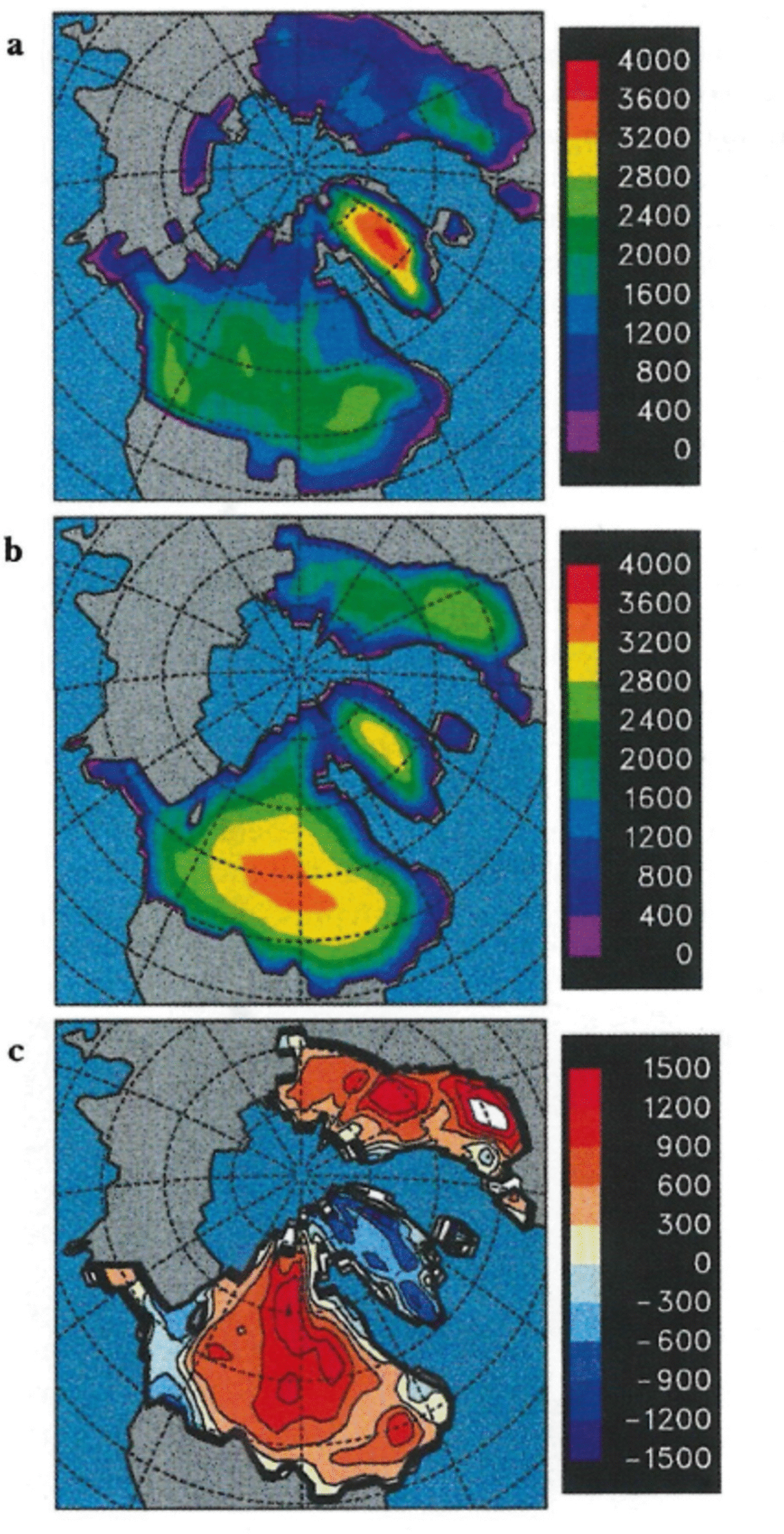
Fig. 3. Ice-sheet topography (before spectral truncation) in ma.s.l.for 21 ka BP Northern Hemispheric ice sheets, (a) ICE-4G ice sheets, (b) CLIMAP ice sheets, (c) Difference (CLIMAP minus ICE-4G).

For our GCM run with CLIMAP ice sheets, SSTs were prescribed from CLIMAP as described above and, except for the ice sheets, the run was identical to the prescribed SST ICE-4G LGM simulation. Figure 4 shows the resulting budgets over the CLIMAP ice sheets. The southern zones of high ablation on the major Northern Hemispheric ice sheets are considerably narrower than for ICE-4G, except for the Cordilleran, the CLIMAP budget of which is even more negative, since its elevations are lower than for ICE-4G. Unlike ICE-4G, there is no obvious “shadow” effect of the CLIMAP Cordilleran on the western Laurentide (in fact, this is a misleading concept since there is no divide separating them in the CLIMAP topography; see Fig. 3b). Despite the higher elevations and steeper flanks, the overall net annual budget for the CLIMAP Laurentide is still –10 cm a^–1 (Table 1), corresponding to a rough time-scale for complete wastage of 25 000 years. This is considerably less negative than the ICE-4G prescribed-SST value of –31 cm a^–1, but still seems implausible, since it implies that the model would not allow a CLIMAP-like Laurentide to expand to its maximum extent in the few thousand years preceding the LGM. For the CLIMAP Eurasian, the annual budget is –5 cm a^–1 (wastage time-scale ∼20 000 years), again considerably less negative than for IGE-4G but still implausible for the LGM. Averaged globally over all CLIMAP ice sheets, the mean budget is –2.2 cm a^–1, corresponding to a sea-level rise of 0.26 cm a^–1.

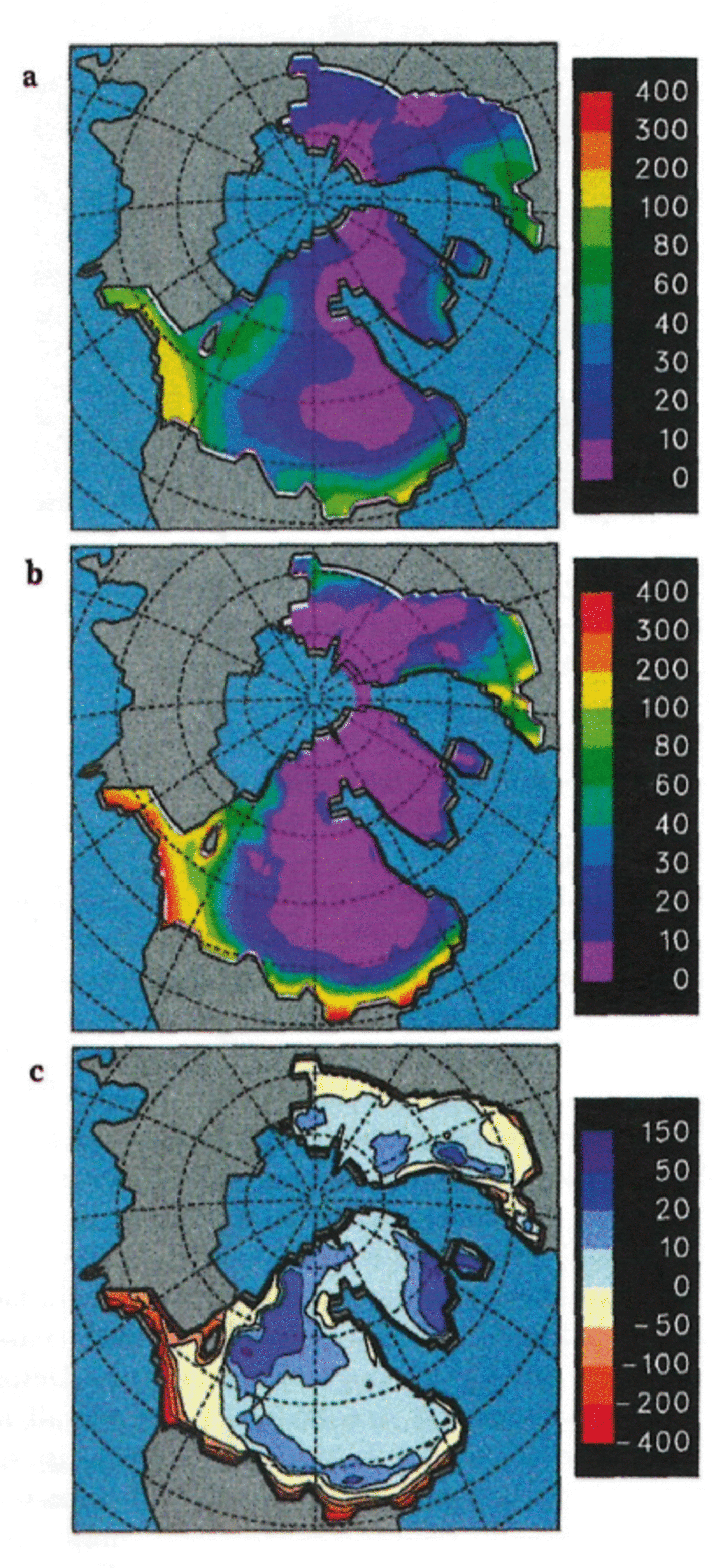
Fig. 4. As Figure 1 except with CLIMAP ice sheets.

Discussion

The central question posed by these ice-sheet budget results is: how could the Laurentide and Eurasian ice sheets have grown out to their maximum observed LGM extents in the interval from about 25-21 ka BP, given the large negative overall budgets simulated by our model for both CLIMAP and ICE-4G ice sheets and for both prescribed CLIMAP and predicted SSTs? One immediate answer is of course that the GCM climate is in error. This is a real possibility, and we will pursue that in the future; also it will be tested as other modern high-resolution GCMs are applied to this problem.

Some of the main uncertainties in the present model are discussed in Reference Pollard and ThompsonPollard and Thompson (in press). However, as discussed in that paper, the 21 ka BP climate of the model compares favorably to a number of other proxy data. And our two current ice-sheet-specific techniques, that correct the relatively coarse-grid GCM meteorology to the icesheet surface, and account for the GCM's neglect of meltwater refreezing, do yield realistic mass balances for present- day ice sheets (Reference Thompson and PollardThompson and Pollard, 1997). That gives us the temerity to imagine (at least for the remainder of this paper) that the GCM physics is more or less correct, and to explore the consequences of our negative LGM icesheet budgets in terms of the prescribed boundary datasets and the basic rationale itself of non-negative budgets at the LGM.

We have only been able to achieve a near-zero ICE-4G Laurentide budget with an unreasonably large imposed cooling of SSTs. Using CLIMAP SSTs and CLIMAP ice sheets, the Laurentide budget is still slightly negative (–10 cm a^–1), but we expect that a further simulation with moderate additional cooling from aerosols (Reference HarveyHarvey, 1988; but see Reference Anderson and CharlsonAnderson and Charlson, 1990), combined with GLIMAP ice sheets and predicted mixed-layer SSTs could yield zero or positive ice budgets, and we are currently preparing to make such a run. Assuming that expectation is true and, if a CLIMAP-like Laurentide ice sheet existed from ∼25–22 ka BP, it could have grown out to the observed southern boundaries at the LGM. But in order to be consistent with the ICE-4G reconstruction at 21 ka BP, such an ice sheet would have had to undergo rapid collapse to the ICE-4G profile just before 21 ka BP.

Is this scenario physically possible? Such a collapse is similar to the surges over deformable thawed beds proposed by Reference MacAyealMacAyeal (1993), Reference ClarkClark (1994, Reference Clark1995) and others. Clark has suggested that surging of the southern periphery of the Laurentide occurred repeatedly during and since the LGM, due to the sedimentary beds underlying the southern parts of the ice sheet south of the Canadian Shield. Surges occurred when these beds warmed to the melting point and became lubricated; at other times they were frozen and could support higher basal-shear stress. So from 25–22 ka BP these southern beds could have been frozen and able to support the steep flanks of a CLIMAP-like ice sheet, and could have become lubricated at about 21 ka BP and induced a sudden collapse of the ICE-4G profile. Immediately following the surgeinduced collapse, the southern portions of the ICE-4G Laurentide would have experienced rapid ablation, and the southern margins would have begun to retreat rapidly.

Is this scenario in obvious conflict with the geologic record? The collapse of such a large volume of ice, if it had flowed into the Gulf of Mexico, should have left a freshwater signal in δ¹⁸O and planktonic foraminifera cores in that region, but no such spikes are evident during that period (Reference Kennett and ShackletonKennett and Shackleton, 1975). However, if most flowed into the North Atlantic, that would coincide with Hcinrich Event H2 (Reference BondBond and others, 1993; Reference BroeckerBroecker, 1994). Global ice-volume records determined from δ¹⁸O cores show a single global ice-volume maximum at 21 ka BP; however, these represent the combined contributions of other ice sheets (notably Antarctica), and the exact timing of the last maximum is smeared by at least 1000–2000 years due to bioturbation. Hence the true maximum volume of the Laurentide could have occurred slightly earlier than 21 ka BP. High-resolution eustatic sea-level curves should have recorded a sudden sea-level rise of several tens of meters corresponding to the difference in the GLIMAP and ICE- 4G Laurentide volumes, but, to date, such records only extend back to about 21 ka BP (Reference FairbanksFairbanks, 1989).

The terrestrial evidence of the margins of the Laurentide are not as well dated as the deep-sea cores, but do suggest the possibility of complex behavior around the LGM; for instance, measured dates of maximum advance or initial retreat vary between 24–14 ka ¹⁴C around the southern and western margins (Reference RuddimanRuddiman and Wright, 1987; Reference ClarkClark, 1994). One consequence of this scenario would be to alter the initial conditions at 21 ka BP assumed for the ICE-4G reconstruction, which were complete isostatic equilibrium of the bedrock depression under the relatively thin ICE-4G ice sheets (Reference PeltierPeltier, 1994). In the above scenario, the initial depression would have been much deeper due to the prior prolonged existence of a much thicker CLIMAP-like ice sheet. Reference Mitrovica and DavisMitrovica and Davis (1995) have shown that similar changes in the assumed initial conditions have significant effects on the subsequent time-dependent ICE-4G results (although they did not analyze the particular scenario suggested here).

The large negative model budgets for the Cordilleran noted above suggest that even with steeper CLIMAP profiles, additional aerosols, and earlier orbits, the Cordilleran could not have grown out to its CLIMAP or ICE-4G extent by 21 ka BP. However, the terrestrial stratigraphic record suggests that the Cordilleran ice sheet was largely non-existent for much of the period from ∼60 ka BP to a few thousand years before the LGM, and did not reach its maximum extent until 15-14 ka ¹⁴C years (18–17 kaBP) (Reference ClarkClark and others, 1993). This would explain our predicted negative Cordilleran budgets, but would leave unexplained how the Cordilleran could then have grown to its maximum size between 21-17 kaBP, while the Laurentide was retreating. (The “shadowing” effect of the ICE-4G Cordilleran noted above suggests that a much smaller Cordilleran prior to 21 ka BP could have allowed more snowfall from the moist westerlies to reach the western and southwestern flanks of the Laurentide, thus aiding the latter's growth to the LGM, and that subsequent growth of the Cordilleran after the LGM could have accelerated retreat of the Laurentide's western sectors (personal communication from P. Clark, 1996).)

We propose the above scenario tentatively, as a possible starting point for exploration of conditions leading up to the LGM. Given the uncertainties inherent in any paleoclimatic GCM simulation, it would be foolhardy to take our simulated negative-ice budgets at face value. But if they do turn out to be robust, and arc confirmed by independent GCM simulations in the future (with higher resolutions, and/or using similar icc-sheet-specific correction techniques to those above), then the question will remain: how could the Laurentide and Eurasian ice sheets have expanded to their maximum extents in the few thousand years leading up to the LGM? Based on the scenario suggested above, we plan to perform additional GCM experiments with (i) additional aerosols, (ii) 25kaBP orbit, (iii) CLIMAP ice-sheet profiles, and (iv) a lowered or non-existent Cordilleran ice sheet to reduce its “shadow” effect on the Laurentide precipitation. If these experiments produce positive mass balances, then it would be worthwhile to perform an asynchronous run spanning the interval ~30-21 ka BP, with the GCM coupled to a 2-D dynamical ice-sheet model (Reference Pollard and ThompsonPollard and Thompson, 1997; Reference Schlesinger and VerbitskySchlesinger and Verbitsky, 1996).