


1. Introduction
Many developed countries in Europe and North America have adopted the unfunded pay-as-you-go (PAYGO) pension system. Due to unexpected and substantial fertility and mortality changes, a lot of them have suffered budgetary difficulties in recent decades. Learning from the experience of these countries, more and more emerging economies opt for the defined-contribution system. At the same time, some developed countries have also reformed their pension system by adding a new (and usually smaller) defined-contribution component [OECD (2021), pp. 49–51]. While the governments adopting this kind of arrangement are less likely to have budgetary problems when facing demographic changes, one disadvantage of this system is that the retirees have to bear more risks, including the longevity risk (the risk of outliving their resources when they live longer than anticipated).
In this context, an important policy debate is whether appropriate financial instruments are available for retirees to insure against longevity risk during the wealth decumulation phase [Mitchell and Piggott (Reference Mitchell, Piggott, Mitchell and Piggott2011)]. In principle, they can rely on the private financial market to hedge this risk. However, it is well known that few individuals purchase annuity products, and, for those who purchase, they only spend a small portion of their wealth on annuities [Modigliani (Reference Modigliani1986), Brown (Reference Brown2001), Benartzi et al. (Reference Benartzi, Previtero and Thaler2011)].
Perhaps because of the retirees’ lack of enthusiasm in participating in the private annuity market, several economies including Denmark, Hong Kong, India, Lithuania, Singapore, and Sweden have introduced the public annuity (PA) plans in recent years. Lau and Zhang (Reference Lau and Zhang2023) summarize the similarities and differences of public annuitization policies in these economies. In particular, there is a major difference among these plans regarding how the retirees are expected to participate: retirees in Hong Kong and India can choose whether to purchase the PA or not, while the participation in the other four economies is mandatory.Footnote 1 Moreover, a simple two-way classification of voluntary versus mandatory plans does not describe very accurately the observed practices that the PA plans in Singapore and Sweden are mandatory but with some flexibility in annuitization choice, while the PA plan in Hong Kong is voluntary but with a restriction on the maximum purchase amount. It is not entirely clear what are the roles of flexibility in a mandatory PA plan and restrictiveness in a voluntary PA plan?
Given these different practices, our first objective is to understand the economic reasons of introducing two observed PA plans: the mandatory public annuity with flexibility (MPAf) and voluntary public annuity with ceiling (VPAc) plans. Another objective is to understand how different retirees are affected if the government decides to introduce a particular PA plan.
We analyze these two PA plans in a model with asymmetric information on survival probability. The model structure is similar to those in existing annuity studies such as Abel (Reference Abel1986) and Brugiavini (Reference Brugiavini1993), but our focus is on the roles of flexibility versus restrictiveness in a mandatory or voluntary PA plan. We obtain two major sets of results. First, when compared with the private annuity payout before the PA plan is introduced, the equilibrium PA payout is higher, but that of the private annuity is lower. Second, we find that the MPAf and VPAc plans have systematically different effects on the welfare of retirees with different survival probabilities. The average health group benefits and the good health group is adversely affected in either the MPAf or VPAc plan. The poor health group benefits from the VPAc plan, but is adversely affected in the MPAf plan.
The underlying reasons of both sets of results are that introducing either PA plan leads to two effects. Because of the quantity restrictions of the PA plan, the severity of adverse selection in public annuities is reduced, leading to a higher equilibrium PA payout. We label it the severity reduction effect. However, this advantage is accompanied by a negative effect of more distortion in the private annuity market, leading to a lower equilibrium private annuity payout. We label it the private market distortion effect. Moreover, when compared with a MPAf plan with the same restriction on the maximum amount of PA purchase, the strength of the severity reduction effect and that of the private market distortion effect in the VPAc plan are both smaller. The interaction of these two effects also explains the systematically different effects on the welfare of distinct groups of retirees. Whether the MPAf or VPAc plan is adopted, the average health group benefits because the severity reduction effect dominates, and the good health group is adversely affected because the private market distortion effect dominates. On the other hand, the impact on the poor health group depends on which PA plan is adopted. In particular, they are adversely affected in the MPAf plan because of the distortion caused by the requirement to buy the minimum mandated level, but benefit from the VPAc plan because the restriction of the maximum purchase does not affect their preferred level of PA purchase.
The rest of this paper is organized as follows. Section 2 provides literature review. Section 3 introduces the model. In Section 4, we examine separately two observed PA plans: the VPAc plan and the MPAf plan. In particular, we study the relative importance of the severity reduction and private market distortion effects in these plans. Section 5 examines the effects of the PA plans on the utility levels of different retirees. Section 6 concludes.
2. Related literature
Our study is related to two strands of the literature. First, it is related to the literature of retirement financing [such as McGrattan and Prescott (Reference McGrattan and Prescott2017), Hosseini and Shourideh (Reference Hosseini and Shourideh2019)]. In particular, our study is related closely to the idea of government-provided annuity during the wealth decumulation phase of retirement financing. In the context of PAYGO system, Diamond (Reference Diamond2004) suggests the idea of government-provided annuity because of the potential efficiency due to economies of scale and lower administrative cost. Fong et al. (Reference Fong, Mitchell and Koh2011) evaluate the money’s worth of the mandatory public annuities offered by the Singaporean government and find that the annuity purchasers benefit from the lower cost of PA provision. They also examine the possible crowding out effect of the government-provided annuities on private annuity providers.
Motivated by recent PA practices, Lau and Zhang (Reference Lau and Zhang2023) examine retirement financing policy questions related to the guarantee and non-escalating payments of the voluntary PA plan. However, the mandatory PA plan and the private annuity market have not been examined in that paper. This paper studies the more fundamental question of voluntary versus mandatory PA plans when the private annuity market is present.
Second, our study is related to the annuity demand literature in the presence of adverse selection. The seminal study of Yaari (Reference Yaari1965) starts the research on annuity demand. Davidoff et al. (Reference Davidoff, Brown and Diamond2005) extend Yaari’s (Reference Yaari1965) analysis by considering weaker conditions. Rothschild and Stiglitz (Reference Rothschild and Stiglitz1976) and Wilson (Reference Wilson1977) examine information asymmetry in the insurance market generally, and Abel (Reference Abel1986) and Eichenbaum and Peled (Reference Eichenbaum and Peled1987) study adverse selection in the annuity market. Subsequently, simulation studies [such as Friedman and Warshawsky (Reference Friedman and Warshawsky1990)] and empirical studies [such as Finkelstein and Poterba (Reference Finkelstein and Poterba2002, Reference Finkelstein and Poterba2004), Einav et al. (Reference Einav, Finkelstein and Schrimpf2010)] support the idea that information asymmetry causes adverse selection in the annuity market.
The major forms of annuity contract discussed in the literature are either non-exclusive contract with linear pricing [Abel (Reference Abel1986), Brugiavini (Reference Brugiavini1993), Hosseini (Reference Hosseini2015)] or exclusive contract specifying both prices and quantities [Eckstein et al. (Reference Eckstein, Eichenbaum and Peled1985), Eichenbaum and Peled (Reference Eichenbaum and Peled1987)]. Motivated by the form of PA contracts offered in various economies, we differ from these studies in one key aspect: we examine the annuities specifying linear price for all buyers but having possible quantity restrictions on the minimum and maximum amounts of purchase. This extension allows us to examine the roles of mandatory and voluntary elements in a PA plan and apply the annuity demand theory to study various empirically relevant PA plans.
3. A model of private and public annuities
In this section, we introduce a simple two-period model of annuity purchase when public and private annuities coexist. In reality, we seldom observe a complete crowding out of the private annuity market by the provision of public annuities.
In the literature, several important factors have been emphasized in understanding annuitization behavior, especially the low level of purchase of private annuities. The factors include high annuity price (which may arise from adverse selection, high administrative cost, etc.), illiquidity concern, intra-family risk sharing, and crowding out effect of government pension. Among them, adverse selection due to asymmetric information on survival probability is a major factor, based on previous theoretical work [such as Eckstein et al. (Reference Eckstein, Eichenbaum and Peled1985); Abel (Reference Abel1986); Hosseini (Reference Hosseini2015)] and empirical studies [such as Finkelstein and Poterba (Reference Finkelstein and Poterba2004); Einav et al. (Reference Einav, Finkelstein and Schrimpf2010)].
Incorporating the above idea, our model contains the feature of information asymmetry on survival probability.Footnote 2 In the following analysis, we first establish the model environment before the PA plan is introduced and then analyze the outcomes after the introduction of various PA plans.
3.1 Asymmetric information on survival probability
We consider a continuum of retirees who live for two periods at most: Period 1 with certainty and Period 2 with some probability ( $\theta$
). The two periods correspond to, respectively, the early and advanced stages of retirement. Retirees have different probabilities of surviving to Period 2, represented by a cumulative distribution
$\theta$
). The two periods correspond to, respectively, the early and advanced stages of retirement. Retirees have different probabilities of surviving to Period 2, represented by a cumulative distribution $F(\theta )$
where
$F(\theta )$
where $\theta \in \lbrack \underline{\theta },\overline{\theta }]$
and
$\theta \in \lbrack \underline{\theta },\overline{\theta }]$
and $0\leq \underline{\theta }< \overline{\theta }\leq 1$
.Footnote
3
Generally, an individual knows her behavior and preference in health-related activities and has a better sense about her health and survival probability. In this model, we assume that
$0\leq \underline{\theta }< \overline{\theta }\leq 1$
.Footnote
3
Generally, an individual knows her behavior and preference in health-related activities and has a better sense about her health and survival probability. In this model, we assume that $\theta$
is private information and is known by the individual in Period 1.
$\theta$
is private information and is known by the individual in Period 1.
We assume that non-exclusive annuity contracts with linear pricing (as in Abel, Reference Abel1986; Hosseini, Reference Hosseini2015), rather than exclusive contracts with price convexity [as in Eckstein et al. (Reference Eckstein, Eichenbaum and Peled1985); Eichenbaum and Peled (Reference Eichenbaum and Peled1987)], are offered, because all observed PA contracts in various economies are similar to this type. Moreover, as pointed out by Abel (Reference Abel1986), it is hard to determine whether a buyer also holds annuities from other providers. This difficulty affects the effectiveness of exclusive contracts in the annuity market.Footnote 4 Motivated by observed practices, we also assume that quantity restrictions are imposed on the public annuities. As will be elaborated in Section 4.3, a distinguishing feature between public and private annuity provision in the presence of adverse selection is the effectiveness of imposing the quantity restrictions.
In the model, the lifetime utility of a retiree with survival probability $\theta$
is given by
$\theta$
is given by
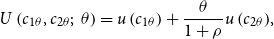 \begin{equation} U\left ( c_{1\theta },c_{2\theta };\,\ \theta \right ) =u\left ( c_{1\theta }\right ) +\frac{\theta }{1+\rho }u\left ( c_{2\theta }\right )\!, \end{equation}
where $c_{i\theta }$
is the level of consumption expenditure in Period
$c_{i\theta }$
is the level of consumption expenditure in Period $i$
(
$i$
( $i=1,2$
) and
$i=1,2$
) and $\rho$
is the subjective discount rate. We assume that the utility function
$\rho$
is the subjective discount rate. We assume that the utility function $U ( c_{1\theta },c_{2\theta };\,\ \theta )$
in (1) is homothetic, with the property that the marginal rate of substitution is a homogeneous function of degree 0:
$U ( c_{1\theta },c_{2\theta };\,\ \theta )$
in (1) is homothetic, with the property that the marginal rate of substitution is a homogeneous function of degree 0:
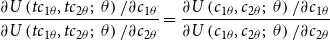 \begin{equation} \frac{\partial U\left ( tc_{1\theta },tc_{2\theta };\,\ \theta \right )/\partial c_{1\theta }}{\partial U\left ( tc_{1\theta },tc_{2\theta };\,\ \theta \right )/\partial c_{2\theta }}=\frac{\partial U\left ( c_{1\theta },c_{2\theta };\,\ \theta \right )/\partial c_{1\theta }}{\partial U\left ( c_{1\theta },c_{2\theta };\,\ \theta \right )/\partial c_{2\theta }} \end{equation}
for $t> 0$
.Footnote
5
Moreover, the standard assumptions that
$t> 0$
.Footnote
5
Moreover, the standard assumptions that $u ( c )$
is strictly concave and
$u ( c )$
is strictly concave and $\lim _{c\rightarrow 0}u^{^{\prime }} ( c ) =\infty$
hold.
$\lim _{c\rightarrow 0}u^{^{\prime }} ( c ) =\infty$
hold.
For simplicity, we do not consider bequest motive in this paper, because it is not likely to be a major factor in understanding the similarities and differences of voluntary versus mandatory PA plans. Assuming away bequest motive means that the annuity always dominates the risk-free bond as the financial tool to hedge longevity risk [e.g. Yaari (Reference Yaari1965), Davidoff et al. (Reference Davidoff, Brown and Diamond2005)]. As a result, retirees do not consider the purchase of risk-free bond in our model.
3.2 Before the introduction of the PA plan
We first consider the outcome before the introduction of the PA plan. A typical retiree makes the consumption and annuitization choices to maximize her expected lifetime utility, given by (1). The outcome under this environment will be useful in subsequent analysis, particularly the analysis (in Section 5) of the impact on different retirees when the government considers whether to adopt a particular PA plan or not.
In this paper, we consider an annuity contract with survival-contingent payments only. The private annuity contract operates as follows. If a retiree buys one dollar of annuity in Period 1, she will receive $\widehat{V}$
dollars in Period 2 if she is alive. With this annuity product, her budget constraints are given by:
$\widehat{V}$
dollars in Period 2 if she is alive. With this annuity product, her budget constraints are given by:
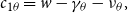
 \begin{equation} \widehat{c}_{1\theta }=w-\widehat{\nu }_{\theta }, \end{equation}
and
 \begin{equation} \widehat{c}_{2\theta }=\widehat{V}\widehat{\nu }_{\theta }, \end{equation}
where $\widehat{\nu }_{\theta }$
is the annuitization amount of a retiree with parameter
$\widehat{\nu }_{\theta }$
is the annuitization amount of a retiree with parameter $\theta$
and
$\theta$
and $w$
is the retiree’s wealth. Since borrowing against annuity contracts is not allowed in most societies, the restriction of non-negative amounts of annuity purchase (
$w$
is the retiree’s wealth. Since borrowing against annuity contracts is not allowed in most societies, the restriction of non-negative amounts of annuity purchase ( $\widehat{\nu }_{\theta }\geq 0$
) is imposed. Note that we use the symbol
$\widehat{\nu }_{\theta }\geq 0$
) is imposed. Note that we use the symbol $^{\wedge}$
above a variable to denote the corresponding variable in the economy before the introduction of the PA (i.e., with private annuity market only).
$^{\wedge}$
above a variable to denote the corresponding variable in the economy before the introduction of the PA (i.e., with private annuity market only).
The annuity buyer’s optimization problem, after knowing her private information $\theta$
, is to choose
$\theta$
, is to choose $\widehat{\nu }_{\theta }$
to maximize
$\widehat{\nu }_{\theta }$
to maximize
 \begin{equation} U\left ( \widehat{c}_{1\theta },\widehat{c}_{2\theta };\,\ \theta \right ) =u\left ( \widehat{c}_{1\theta }\right ) +\frac{\theta }{1+\rho }u\left ( \widehat{c}_{2\theta }\right ) =u\left ( w-\widehat{\nu }_{\theta }\right ) +\frac{\theta }{1+\rho }u\left ( \widehat{V}\widehat{\nu }_{\theta }\right ). \end{equation}
It is easy to show that the optimal choice of $\widehat{\nu }_{\theta }$
is an interior solution, which is characterized by:Footnote
6
$\widehat{\nu }_{\theta }$
is an interior solution, which is characterized by:Footnote
6
 \begin{equation} u^{\prime }\left ( w-\widehat{\nu }_{\theta }^{\ast }\right ) =\frac{\theta }{1+\rho }\widehat{V}u^{\prime }\left ( \widehat{V}\widehat{\nu }_{\theta }^{\ast }\right ), \end{equation}
where the symbol * associated with a variable denotes the optimal choice of that variable.
The left-hand side (LHS) in the first-order condition (6) is the marginal cost of annuitizing one more dollar, because the buyer has to reduce one unit of consumption in Period 1. In terms of utility, the marginal cost is $u^{\prime } ( \widehat{c}_{1\theta }^{\ast } ) =u^{\prime } ( w-\widehat{\nu }_{\theta }^{\ast } )$
. If the buyer is alive in Period 2, she receives
$u^{\prime } ( \widehat{c}_{1\theta }^{\ast } ) =u^{\prime } ( w-\widehat{\nu }_{\theta }^{\ast } )$
. If the buyer is alive in Period 2, she receives $\widehat{V}$
extra units of annuity income. Thus, the increase in her utility level is given by
$\widehat{V}$
extra units of annuity income. Thus, the increase in her utility level is given by $\widehat{V}u^{\prime } ( \widehat{c}_{2\theta }^{\ast } ) =\widehat{V}u^{\prime } ( \widehat{V}\widehat{\nu }_{\theta }^{\ast } )$
. After discounting the expected value of this future utility benefit back to Period 1, we have the right-hand side (RHS) term of (6). At the optimal choice, the marginal benefit and marginal cost are equal according to (6).
$\widehat{V}u^{\prime } ( \widehat{c}_{2\theta }^{\ast } ) =\widehat{V}u^{\prime } ( \widehat{V}\widehat{\nu }_{\theta }^{\ast } )$
. After discounting the expected value of this future utility benefit back to Period 1, we have the right-hand side (RHS) term of (6). At the optimal choice, the marginal benefit and marginal cost are equal according to (6).
Differentiating (6) totally, we obtain
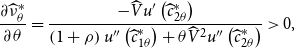 \begin{equation} \frac{\partial \widehat{\nu }_{\theta }^{\ast }}{\partial \theta }=\frac{-\widehat{V}u^{\prime }\left ( \widehat{c}_{2\theta }^{\ast }\right ) }{\left ( 1+\rho \right ) u^{\prime \prime }\left ( \widehat{c}_{1\theta }^{\ast }\right ) +\theta \widehat{V}^{2}u^{\prime \prime }\left ( \widehat{c}_{2\theta }^{\ast }\right ) }> 0, \end{equation}
which suggests that the optimal annuity choice $\widehat{v}_{\theta }^{\ast }$
is increasing in the survival probability
$\widehat{v}_{\theta }^{\ast }$
is increasing in the survival probability $\theta$
. The relationship is shown in Panel A of Figure 1.
$\theta$
. The relationship is shown in Panel A of Figure 1.
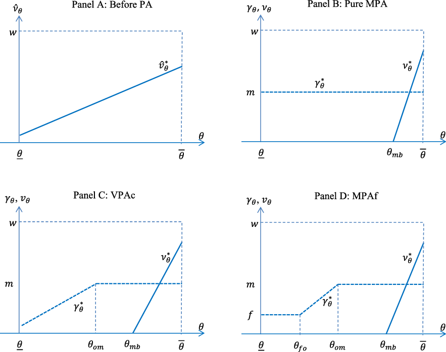
Figure 1. Annuity choices under various plans.
Based on the buyers’ choices described above, annuity providers’ revenue in Period 1 is given by $\int _{\underline{\theta }}^{\overline{\theta }}\widehat{\nu }_{\theta }^{\ast }dF(\theta )$
, and their expected payment in Period 2 is
$\int _{\underline{\theta }}^{\overline{\theta }}\widehat{\nu }_{\theta }^{\ast }dF(\theta )$
, and their expected payment in Period 2 is $\int _{\underline{\theta }}^{\overline{\theta }}\theta \widehat{V}^{\ast }\widehat{\nu }_{\theta }^{\ast }dF(\theta )$
. Following many researchers [such as Abel (Reference Abel1986), Hosseini (Reference Hosseini2015)], we assume the zero-profit condition for the provision of annuities. This assumption offers the advantage that the correlation between survival probability and annuity purchase, which is the source of adverse selection, is reflected in the equilibrium annuity payout level. Under the zero-profit condition for private annuity market, the equilibrium value of the payout term
$\int _{\underline{\theta }}^{\overline{\theta }}\theta \widehat{V}^{\ast }\widehat{\nu }_{\theta }^{\ast }dF(\theta )$
. Following many researchers [such as Abel (Reference Abel1986), Hosseini (Reference Hosseini2015)], we assume the zero-profit condition for the provision of annuities. This assumption offers the advantage that the correlation between survival probability and annuity purchase, which is the source of adverse selection, is reflected in the equilibrium annuity payout level. Under the zero-profit condition for private annuity market, the equilibrium value of the payout term $\widehat{V}$
, denoted by
$\widehat{V}$
, denoted by $\widehat{V}^{\ast }$
, is determined according to
$\widehat{V}^{\ast }$
, is determined according to
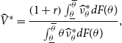 \begin{equation} \widehat{V}^{\ast }=\frac{\left ( 1+r\right ) \int _{\underline{\theta }}^{\overline{\theta }}\widehat{\nu }_{\theta }^{\ast }dF(\theta )}{\int _{\underline{\theta }}^{\overline{\theta }}\theta \widehat{\nu }_{\theta }^{\ast }dF(\theta )}, \end{equation}
after using the discount factor $1/(1+r)$
to adjust for the revenue and payment terms in the two different periods, where
$1/(1+r)$
to adjust for the revenue and payment terms in the two different periods, where $r$
is the interest rate.Footnote
7
According to Lau et al. (Reference Lau, Ying and Zhang2022), the equilibrium payout
$r$
is the interest rate.Footnote
7
According to Lau et al. (Reference Lau, Ying and Zhang2022), the equilibrium payout $\widehat{V}^{\ast }$
is unique for all time-separable utility functions (1) if the distribution of retirees’ survival probabilities satisfies a rather weak condition. For example, a uniform distribution or a truncated normal distribution (
$\widehat{V}^{\ast }$
is unique for all time-separable utility functions (1) if the distribution of retirees’ survival probabilities satisfies a rather weak condition. For example, a uniform distribution or a truncated normal distribution ( $\underline{\theta }\leq \theta \leq \overline{\theta }$
) with variance larger than some threshold level satisfies this sufficient condition.
$\underline{\theta }\leq \theta \leq \overline{\theta }$
) with variance larger than some threshold level satisfies this sufficient condition.
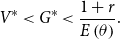
Comparing the payout $\widehat{V}^{\ast }$
with the actuarially fair payout
$\widehat{V}^{\ast }$
with the actuarially fair payout $\frac{1+r}{E\left ( \theta \right ) }$
based on average survival probability of the population, it is straightforward to conclude that
$\frac{1+r}{E\left ( \theta \right ) }$
based on average survival probability of the population, it is straightforward to conclude that
 \begin{equation} \widehat{V}^{\ast }< \frac{1+r}{E\left ( \theta \right ) }, \end{equation}
because $\widehat{\nu }_{\theta }^{\ast }$
and
$\widehat{\nu }_{\theta }^{\ast }$
and $\theta$
are positively correlated according to (7).
$\theta$
are positively correlated according to (7).
The value of payout $\widehat{V}^{\ast }$
is below the actuarially fair level, indicating some efficiency loss due to adverse selection, which is often cited as an important reason calling for government intervention.
$\widehat{V}^{\ast }$
is below the actuarially fair level, indicating some efficiency loss due to adverse selection, which is often cited as an important reason calling for government intervention.
3.3 Introducing the PA plan
In the presence of market imperfection such as adverse selection, the government may choose to intervene in the annuity market in different ways, such as taxation, regulation, or annuity provision. Drawing on the PA practices in various economies [see, e.g. Section 2 and Table 1 of Lau and Zhang (Reference Lau and Zhang2023)], we consider the case that the government (directly or indirectly through a statutory body) steps in the market as the PA provider.
We assume that the PA contract provides survival-contingent payments only. If a retiree buys one dollar of the PA in Period 1, she will receive $G$
dollars in Period 2 if she is alive. Therefore, the retiree’s budget constraints, when both private and public annuities are available, are given by
$G$
dollars in Period 2 if she is alive. Therefore, the retiree’s budget constraints, when both private and public annuities are available, are given by
 \begin{equation} c_{1\theta }=w-\gamma _{\theta }-\nu _{\theta }, \end{equation}
and
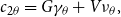 \begin{equation} c_{2\theta }=G\gamma _{\theta }+V\nu _{\theta }, \end{equation}
where $\gamma _{\theta }$
(
$\gamma _{\theta }$
( $\gamma _{\theta }\geq 0$
) is her purchase amount of PA and
$\gamma _{\theta }\geq 0$
) is her purchase amount of PA and $\nu _{\theta }$
(
$\nu _{\theta }$
( $\nu _{\theta }\geq 0$
) is her purchase amount of private annuity. The other variables are the same as before, except that the symbol
$\nu _{\theta }\geq 0$
) is her purchase amount of private annuity. The other variables are the same as before, except that the symbol $^{\wedge}$
is absent after the PA plan is introduced.
$^{\wedge}$
is absent after the PA plan is introduced.
Combining (1), (10), and (11), the problem becomes
 \begin{equation*} \max _{\gamma _{\theta },\nu _{\theta }}U\left ( c_{1\theta },c_{2\theta };\,\ \theta \right ) =u\left ( w-\gamma _{\theta }-\nu _{\theta }\right ) +\frac {\theta }{1+\rho }u\left ( G\gamma _{\theta }+V\nu _{\theta }\right ). \end{equation*}
Solving the above problem leads to the following two conditions:
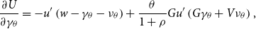 \begin{equation} \frac{\partial U}{\partial \gamma _{\theta }}=-u^{\prime }\left ( w-\gamma _{\theta }-\nu _{\theta }\right ) +\frac{\theta }{1+\rho }Gu^{\prime }\left ( G\gamma _{\theta }+V\nu _{\theta }\right ), \end{equation}
and
 \begin{equation} \frac{\partial U}{\partial \nu _{\theta }}=-u^{\prime }\left ( w-\gamma _{\theta }-\nu _{\theta }\right ) +\frac{\theta }{1+\rho }Vu^{\prime }\left ( G\gamma _{\theta }+V\nu _{\theta }\right ), \end{equation}
where $u^{\prime } ( w-\gamma _{\theta }-\nu _{\theta } )$
in either (12) or (13) is the marginal cost of buying one more unit of a public or private annuity. On the other hand, the marginal benefit of buying a private annuity is different from that of buying the PA, with
$u^{\prime } ( w-\gamma _{\theta }-\nu _{\theta } )$
in either (12) or (13) is the marginal cost of buying one more unit of a public or private annuity. On the other hand, the marginal benefit of buying a private annuity is different from that of buying the PA, with $\frac{\theta }{1+\rho }Gu^{\prime }\left ( G\gamma _{\theta }+V\nu _{\theta }\right )$
in (12) being the marginal benefit of buying the PA, and
$\frac{\theta }{1+\rho }Gu^{\prime }\left ( G\gamma _{\theta }+V\nu _{\theta }\right )$
in (12) being the marginal benefit of buying the PA, and $\frac{\theta }{1+\rho }Vu^{\prime }\left ( G\gamma _{\theta }+V\nu _{\theta }\right )$
in (13) being the marginal benefit of buying the private annuity.
$\frac{\theta }{1+\rho }Vu^{\prime }\left ( G\gamma _{\theta }+V\nu _{\theta }\right )$
in (13) being the marginal benefit of buying the private annuity.
3.4 Pure mandatory PA plan
Before analyzing two PA plans which are empirically relevant, we first consider a benchmark case of a pure mandatory public annuity plan (pure MPA plan) in which all retirees are required to purchase the same level of PA. The results of this case, together with those in the opposite extreme case of a pure VPA plan,Footnote 8 are helpful to understand the similarities and differences of the two PA plans to be considered in the next section.
The pure MPA plan is represented by
 \begin{equation} \gamma _{\theta }=m. \end{equation}
For this plan, the behavior of PA purchase is straightforward, as all retirees are required to buy the same amount ( $m$
) of public annuities. On the other hand, the behavior in the private annuity market is more interesting, particularly when
$m$
) of public annuities. On the other hand, the behavior in the private annuity market is more interesting, particularly when $m$
is set at a not-too-high level such that retirees with high value of
$m$
is set at a not-too-high level such that retirees with high value of $\theta$
still have residual annuitization demand after purchasing the mandated amount of public annuities. In this case, retirees with good health satisfy their residual demands by purchasing annuities from the private sector. The optimal choice of private annuity (
$\theta$
still have residual annuitization demand after purchasing the mandated amount of public annuities. In this case, retirees with good health satisfy their residual demands by purchasing annuities from the private sector. The optimal choice of private annuity ( $\nu _{\theta }^{\ast }$
), which is obtained by combining (14) and
$\nu _{\theta }^{\ast }$
), which is obtained by combining (14) and $\left. \frac{\partial U}{\partial \nu _{\theta }}\right \vert _{\nu _{\theta }=\nu _{\theta }^{\ast }}=0$
in (13), is given by
$\left. \frac{\partial U}{\partial \nu _{\theta }}\right \vert _{\nu _{\theta }=\nu _{\theta }^{\ast }}=0$
in (13), is given by
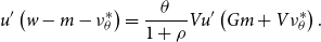 \begin{equation} u^{\prime }\left ( w-m-\nu _{\theta }^{\ast }\right ) =\frac{\theta }{1+\rho }Vu^{\prime }\left ( Gm+V\nu _{\theta }^{\ast }\right ). \end{equation}
Using similar procedure as in (7), we can show that
 \begin{equation} \frac{\partial \nu _{\theta }^{\ast }}{\partial \theta }> 0. \end{equation}
Since $\nu _{\theta }^{\ast }$
is always increasing for those who buy private annuity, we can determine the threshold level of survival probability
$\nu _{\theta }^{\ast }$
is always increasing for those who buy private annuity, we can determine the threshold level of survival probability $\theta _{mb}$
by substituting
$\theta _{mb}$
by substituting $\nu _{\theta }^{\ast }=0$
in (15) to obtain
$\nu _{\theta }^{\ast }=0$
in (15) to obtain
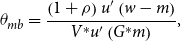 \begin{equation} \theta _{mb}=\frac{\left ( 1+\rho \right ) u^{\prime }\left ( w-m\right ) }{V^{\ast }u^{\prime }\left ( G^{\ast }m\right ) }, \end{equation}
where $V^{\ast }$
is the equilibrium value of payout of the private annuity, which is determined according to the zero-profit condition as
$V^{\ast }$
is the equilibrium value of payout of the private annuity, which is determined according to the zero-profit condition as
 \begin{equation} V^{\ast }=\frac{\left ( 1+r\right ) \int _{\underline{\theta }}^{\overline{\theta }}\nu _{\theta }^{\ast }dF(\theta )}{\int _{\underline{\theta }}^{\overline{\theta }}\theta \nu _{\theta }^{\ast }dF(\theta )}=\frac{\left ( 1+r\right ) \int _{\theta _{mb}}^{\overline{\theta }}\nu _{\theta }^{\ast }dF(\theta )}{\int _{\theta _{mb}}^{\overline{\theta }}\theta \nu _{\theta }^{\ast }dF(\theta )}. \end{equation}
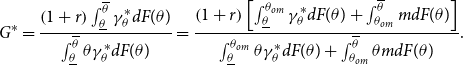
It is straightforward to see that the equilibrium value of PA payout ( $G^{\ast }$
) for the pure MPA plan under the zero-profit condition is given byFootnote
9
$G^{\ast }$
) for the pure MPA plan under the zero-profit condition is given byFootnote
9
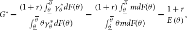 \begin{equation} G^{\ast }=\frac{\left ( 1+r\right ) \int _{\underline{\theta }}^{\overline{\theta }}\gamma _{\theta }^{\ast }dF(\theta )}{\int _{\underline{\theta }}^{\overline{\theta }}\theta \gamma _{\theta }^{\ast }dF(\theta )}=\frac{\left ( 1+r\right ) \int _{\underline{\theta }}^{\overline{\theta }}mdF(\theta )}{\int _{\underline{\theta }}^{\overline{\theta }}\theta mdF(\theta )}=\frac{1+r}{E\left ( \theta \right ) }, \end{equation}
the actuarially fair level.
Buyers’ choices after the introduction of the pure MPA plan are summarized as follows. Buyers with $\theta \leq \theta _{mb}$
purchase the PA (
$\theta \leq \theta _{mb}$
purchase the PA ( $\gamma _{\theta }^{\ast }=m$
) only, where
$\gamma _{\theta }^{\ast }=m$
) only, where $\theta _{mb}$
is defined in (17). On the other hand, buyers with
$\theta _{mb}$
is defined in (17). On the other hand, buyers with $\theta > \theta _{mb}$
purchase both the PA (at the mandated amount,
$\theta > \theta _{mb}$
purchase both the PA (at the mandated amount, $\gamma _{\theta }^{\ast }=m$
) and the private annuity (
$\gamma _{\theta }^{\ast }=m$
) and the private annuity ( $\nu _{\theta }^{\ast }$
), where
$\nu _{\theta }^{\ast }$
), where $\nu _{\theta }^{\ast }$
is determined according to (15) and is increasing in
$\nu _{\theta }^{\ast }$
is determined according to (15) and is increasing in $\theta$
.
$\theta$
.
Buyers’ annuitization choices under the pure MPA plan are shown in Panel B of Figure 1.
4. Two observed PA plans
While analyzing the pure mandatory PA and pure voluntary PA plans allows us to obtain some interesting results, these two plans are less relevant because they are not commonly observed, as we have briefly described in Section 1. In existing voluntary PA plans, there is a restriction on the maximum amount of purchase. Presumably, the PA provider wants to exercise financial prudence to ensure that some buyers, particularly those who are likely to live very long, would not be able to purchase a substantial amount of the PA. On the other hand, there are some elements of flexibility in existing mandatory PA plans, perhaps because the presence of some factors (such as the concern about whether the annuity buyers can afford to purchase the mandated level) makes a uniform mandated level of annuity purchase undesirable for the retirees.
We now analyze buyers’ behavior under two empirically relevant PA plans: a voluntary plan with a restriction on the maximum amount of purchase and a mandatory plan with flexibility.
4.1 VPA plan with ceiling
The Hong Kong Mortgage Corporation (HKMC) Annuity Plan was first launched in July 2018. The plan is a voluntary one. Individuals over a certain age (60 currently) are allowed to purchase the public annuities, with the amount of purchase ranging from HKD50,000 (roughly USD6,400) to a level set by the PA provider from time to time. Currently, the maximum amount of purchase is HKD5 million (roughly USD641,000), which was set at June 2022.Footnote 10
Motivated by the observed practices in Hong Kong, we consider the VPA plan with ceiling, which is specified as:Footnote 11
 \begin{equation} 0\leq \gamma _{\theta }\leq m, \end{equation}
where
 \begin{equation} m\leq \overline{m}, \end{equation}
with $\overline{m}$
being determined according toFootnote
12
$\overline{m}$
being determined according toFootnote
12
 \begin{equation} u^{\prime }\left ( w-\frac{G^{\ast }-V^{\ast }}{\widehat{V}^{\ast }-V^{\ast }}\overline{m}\right ) =\frac{\overline{\theta }}{1+\rho }V^{\ast }u^{\prime }\left ( \widehat{V}^{\ast }\frac{G^{\ast }-V^{\ast }}{\widehat{V}^{\ast }-V^{\ast }}\overline{m}\right ), \end{equation}
and $V^{\ast }$
is determined according to (18) and
$V^{\ast }$
is determined according to (18) and $G^{\ast }$
is the equilibrium payout of the VPAc plan, given by (26) below. Since setting a very high level of
$G^{\ast }$
is the equilibrium payout of the VPAc plan, given by (26) below. Since setting a very high level of $m$
may not be financially prudent and may lead to a complete or substantial crowding out of the private annuity market, it is not likely that many governments want to do so. As will be shown in subsequent analysis, imposing the not-too-high ceiling condition (21) ensures that the private annuity market is not substantially crowded out.
$m$
may not be financially prudent and may lead to a complete or substantial crowding out of the private annuity market, it is not likely that many governments want to do so. As will be shown in subsequent analysis, imposing the not-too-high ceiling condition (21) ensures that the private annuity market is not substantially crowded out.
When the payout of the PA is higher than that of the private annuity (to be shown in Proposition 1) and when the optimal amount of PA purchased by individual $\theta$
, denoted by
$\theta$
, denoted by $\gamma _{\theta }^{\ast }$
, is less than the ceiling level
$\gamma _{\theta }^{\ast }$
, is less than the ceiling level $m$
, the optimal choice
$m$
, the optimal choice $\gamma _{\theta }^{\ast }$
is defined by
$\gamma _{\theta }^{\ast }$
is defined by
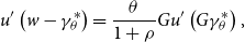 \begin{equation} u^{\prime }\left ( w-\gamma _{\theta }^{\ast }\right ) =\frac{\theta }{1+\rho }Gu^{\prime }\left ( G\gamma _{\theta }^{\ast }\right ), \end{equation}
which is obtained by combining $\nu _{\theta }=0$
and
$\nu _{\theta }=0$
and $\left. \frac{\partial U_{\theta }}{\partial \gamma _{\theta }}\right | _{\gamma _{\theta }=\gamma _{\theta }^{\ast }}=0$
in (12). Following similar procedure as in (7), it is straightforward to show that
$\left. \frac{\partial U_{\theta }}{\partial \gamma _{\theta }}\right | _{\gamma _{\theta }=\gamma _{\theta }^{\ast }}=0$
in (12). Following similar procedure as in (7), it is straightforward to show that
 \begin{equation} \frac{\partial \gamma _{\theta }^{\ast }}{\partial \theta }=\frac{-Gu^{\prime }\left ( c_{2\theta }^{\ast }\right ) }{\left ( 1+\rho \right ) u^{\prime \prime }\left ( c_{1\theta }^{\ast }\right ) +\theta G^{2}u^{\prime \prime }\left ( c_{2\theta }^{\ast }\right ) }> 0. \end{equation}
Buyers’ choices under the VPAc plan are summarized as follows. When this plan is introduced, (a) buyers with $\theta < \theta _{om}$
purchase the PA only, with the PA purchase (
$\theta < \theta _{om}$
purchase the PA only, with the PA purchase ( $\gamma _{\theta }^{\ast }$
) being determined according to (23) and increasing in
$\gamma _{\theta }^{\ast }$
) being determined according to (23) and increasing in $\theta$
, where
$\theta$
, where
 \begin{equation} \theta _{om}=\frac{\left ( 1+\rho \right ) u^{\prime }\left ( w-m\right ) }{G^{\ast }u^{\prime }\left ( G^{\ast }m\right ) }; \end{equation}
(b) buyers with $\theta _{om}\leq \theta \leq \theta _{mb}$
purchase the PA only, and purchase the maximum amount of PA (
$\theta _{om}\leq \theta \leq \theta _{mb}$
purchase the PA only, and purchase the maximum amount of PA ( $\gamma _{\theta }^{\ast }=m$
), where
$\gamma _{\theta }^{\ast }=m$
), where $\theta _{mb}$
is defined in (17); and (c) buyers with
$\theta _{mb}$
is defined in (17); and (c) buyers with $\theta > \theta _{mb}$
purchase both the PA (at the maximum amount,
$\theta > \theta _{mb}$
purchase both the PA (at the maximum amount, $\gamma _{\theta }^{\ast }=m$
) and the private annuity (
$\gamma _{\theta }^{\ast }=m$
) and the private annuity ( $\nu _{\theta }^{\ast }$
), with
$\nu _{\theta }^{\ast }$
), with $\nu _{\theta }^{\ast }$
being determined according to (15) and increasing in
$\nu _{\theta }^{\ast }$
being determined according to (15) and increasing in $\theta$
. (The proof of the above results, which is straightforward but tedious, is given in the Online Appendix.)
$\theta$
. (The proof of the above results, which is straightforward but tedious, is given in the Online Appendix.)
Consistent with the buyers’ behavior, the equilibrium value of PA payout of the VPAc plan is given byFootnote 13
 \begin{equation} G^{\ast }=\frac{\left ( 1+r\right ) \int _{\underline{\theta }}^{\overline{\theta }}\gamma _{\theta }^{\ast }dF(\theta )}{\int _{\underline{\theta }}^{\overline{\theta }}\theta \gamma _{\theta }^{\ast }dF(\theta )}=\frac{\left ( 1+r\right ) \left [ \int _{\underline{\theta }}^{\theta _{om}}\gamma _{\theta }^{\ast }dF(\theta )+\int _{\theta _{om}}^{\overline{\theta }}mdF(\theta )\right ] }{\int _{\underline{\theta }}^{\theta _{om}}\theta \gamma _{\theta }^{\ast }dF(\theta )+\int _{\theta _{om}}^{\overline{\theta }}\theta mdF(\theta )}. \end{equation}
Buyers’ annuitization choices under the VPAc plan are shown in Panel C of Figure 1.
4.2 MPA plan with flexibility
The Central Provident Fund (CPF) Lifelong Income for the Elderly (LIFE) program in Singapore was introduced in 2009 and has become mandatory since 2013. Participants are required to set aside the Full Retirement Sum (FRS) to buy the lifelong annuity provided by the CPF Board. The FRS level is adjusted periodically and the current level is, for example, 192,000 Singaporean dollars (about USD142,000) for those aged 55 in 2022. In 2016, the CPF Board introduced the Retirement Sum Topping-Up Scheme. Participants can use this scheme to top-up their Retirement Sum up to the Enhanced Retirement Sum (ERS), which is 1.5 times of the FRS.Footnote 14 We observe that a floor (i.e. the FRS) and a ceiling (i.e. the ERS) are imposed on the amount of PA purchase in the CPF LIFE plan. Some flexibility between these two levels is given to the participants in this MPA program.
Motivated by the observed practices in Singapore,Footnote 15 the MPA plan with flexibility is specified as:
 \begin{equation} f\leq \gamma _{\theta }\leq m, \end{equation}
where parameters $m$
and
$m$
and $f$
satisfy (21) andFootnote
16
$f$
satisfy (21) andFootnote
16
 \begin{equation} \widehat{\nu }_{\underline{\theta }}^{\ast }\leq f< m. \end{equation}
If condition (28) does not hold, the lowest mandated level ( $f$
) of the MPAf plan is even lower than the purchase level of private annuity of the least healthy retiree before the PA plan is introduced. We impose condition (28) to eliminate this uninteresting case.Footnote
17
$f$
) of the MPAf plan is even lower than the purchase level of private annuity of the least healthy retiree before the PA plan is introduced. We impose condition (28) to eliminate this uninteresting case.Footnote
17
Following similar procedure as above, buyer’s behavior under this PA plan is given as follows. After the PA plan is introduced, (a) buyers with $\theta \leq \theta _{fo}$
only purchase the minimum required level (
$\theta \leq \theta _{fo}$
only purchase the minimum required level ( $\gamma _{\theta }^{\ast }=f$
) of PA, where
$\gamma _{\theta }^{\ast }=f$
) of PA, where
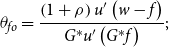 \begin{equation} \theta _{fo}=\frac{\left ( 1+\rho \right ) u^{\prime }\left ( w-f\right ) }{G^{\ast }u^{\prime }\left ( G^{\ast }f\right ) }; \end{equation}
(b) buyers with $\theta _{fo}< \theta < \theta _{om}$
purchase the PA only, with the PA purchase (
$\theta _{fo}< \theta < \theta _{om}$
purchase the PA only, with the PA purchase ( $\gamma _{\theta }^{\ast }$
) being determined according to (23) and increasing in
$\gamma _{\theta }^{\ast }$
) being determined according to (23) and increasing in $\theta$
, where
$\theta$
, where $\theta _{om}$
is defined in (25); (c) buyers with
$\theta _{om}$
is defined in (25); (c) buyers with $\theta _{om}\leq \theta \leq \theta _{mb}$
purchase the maximum amount of PA (
$\theta _{om}\leq \theta \leq \theta _{mb}$
purchase the maximum amount of PA ( $\gamma _{\theta }^{\ast }=m$
) only, where
$\gamma _{\theta }^{\ast }=m$
) only, where $\theta _{mb}$
is defined in (17); and (d) buyers with
$\theta _{mb}$
is defined in (17); and (d) buyers with $\theta > \theta _{mb}$
purchase both the PA (at the maximum amount,
$\theta > \theta _{mb}$
purchase both the PA (at the maximum amount, $\gamma _{\theta }^{\ast }=m$
) and the private annuity (
$\gamma _{\theta }^{\ast }=m$
) and the private annuity ( $\nu _{\theta }^{\ast }$
), with
$\nu _{\theta }^{\ast }$
), with $\nu _{\theta }^{\ast }$
being determined according to (15) and increasing in
$\nu _{\theta }^{\ast }$
being determined according to (15) and increasing in $\theta$
. Moreover, the equilibrium PA payout of the MPAf plan is given by
$\theta$
. Moreover, the equilibrium PA payout of the MPAf plan is given by
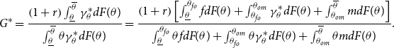 \begin{equation} G^{\ast }=\frac{\left ( 1+r\right ) \int _{\underline{\theta }}^{\overline{\theta }}\gamma _{\theta }^{\ast }dF(\theta )}{\int _{\underline{\theta }}^{\overline{\theta }}\theta \gamma _{\theta }^{\ast }dF(\theta )}=\frac{\left ( 1+r\right ) \left [ \int _{\underline{\theta }}^{\theta _{fo}}fdF(\theta )+\int _{\theta _{fo}}^{\theta _{om}}\gamma _{\theta }^{\ast }dF(\theta )+\int _{\theta _{om}}^{\overline{\theta }}mdF(\theta )\right ] }{\int _{\underline{\theta }}^{\theta _{fo}}\theta fdF(\theta )+\int _{\theta _{fo}}^{\theta _{om}}\theta \gamma _{\theta }^{\ast }dF(\theta )+\int _{\theta _{om}}^{\overline{\theta }}\theta mdF(\theta )}. \end{equation}
Buyers’ annuitization choices under the MPAf plan are shown in Panel D of Figure 1.
4.3 Severity reduction and private market distortion effects in a two-tier annuity market
In Sections 4.1 and 4.2, we obtained the results about annuity buyers’ choices conditional on a higher payout for the PA ( $G^{\ast }> V^{\ast }$
). The following proposition, which compares each of the equilibrium payouts of the public and private annuities with the payout level of the private annuity market before the PA plan is introduced, confirms that
$G^{\ast }> V^{\ast }$
). The following proposition, which compares each of the equilibrium payouts of the public and private annuities with the payout level of the private annuity market before the PA plan is introduced, confirms that $G^{\ast }> V^{\ast }$
is an endogenous outcome under either the VPAc or MPAf plan.Footnote
18
$G^{\ast }> V^{\ast }$
is an endogenous outcome under either the VPAc or MPAf plan.Footnote
18
Proposition 1. Consider the introduction of either the VPAc plan or MPAf plan. Compared with the equilibrium payout of the private annuity ( $\widehat{V}^{\ast }$
) before the introduction of the PA plan,
$\widehat{V}^{\ast }$
) before the introduction of the PA plan,
(a) the equilibrium payout of the PA is higher:
 \begin{equation} G^{\ast }> \widehat{V}^{\ast }; \end{equation}
and (b) the equilibrium payout of the private annuity is lower:
 \begin{equation} V^{\ast }< \widehat{V}^{\ast }. \end{equation}
Proof. See Appendix A.
Combining parts (a) and (b) of Proposition 1, together with the positive correlation of the annuity purchase amount and $\theta$
according to (24) for those buyers whose purchase amounts are not constrained by the quantity restrictions of the PA plan, we obtainFootnote
19
$\theta$
according to (24) for those buyers whose purchase amounts are not constrained by the quantity restrictions of the PA plan, we obtainFootnote
19
 \begin{equation} V^{\ast }< G^{\ast }< \frac{1+r}{E\left ( \theta \right ) }. \end{equation}
An implication of (33) is the outcome of a two-tier annuity market. Less healthy people only purchase the public annuities, but healthier people purchase both public and private annuities. Moreover, we observe from the above analysis that there are two key effects when the PA plan is introduced.
First, the design of the PA plan matters. The imposed quantity restrictions (for both the ceiling and floor) on the PA purchase lead to a reduction in the severity of adverse selection, which originally arises from the positive correlation of the risk type (based on survival probability) and the PA purchase amount. Specifically, the ceiling restriction of both PA plans reduces the positive correlation of these two variables at the upper end by restricting the purchase amount of healthier retirees to the maximum level ( $m$
), and the floor restriction of the MPAf plan reduces the positive correlation at the lower end by requiring the less healthy retirees to purchase the minimum mandated level (
$m$
), and the floor restriction of the MPAf plan reduces the positive correlation at the lower end by requiring the less healthy retirees to purchase the minimum mandated level ( $f$
). We call this effect the severity reduction effect.
$f$
). We call this effect the severity reduction effect.
The restrictions imposed by the PA plans may not be implemented in the private annuity market, and even if some of them are implemented, the effects are different. Obviously, private annuity companies cannot make retirees’ purchase of private annuity products mandatory. On the other hand, imposing the maximum purchase level is possible for private annuity companies, but this policy is not effective in reducing the severity of adverse selection of the competitive private market. In a competitive market where different companies offer similar annuity products, if a company sets a purchase ceiling, a retiree with good health can buy the maximum amount from this company and then go to another one to satisfy her unfulfilled demand. It is not likely (and also not legal in many countries) that different companies share their customer lists and restrict the customers from going to other companies to buy annuities.Footnote 20 Since the overall severity of adverse selection is determined by the total amount of private annuity purchased by all retirees, the effect of imposing purchase restriction on the severity of adverse selection in the PA sector cannot be replicated in the private market.
Second, the PA plan affects indirectly the private annuity market. Since the public and private annuity contracts provide the same financial function to the retirees, and the payout of the PA is higher, the retirees satisfy their annuity demand by first purchasing the more attractive PA. Because of the restrictions imposed by either VPAc or MPAf plan, the demands of some retirees may not be completely satisfied. As shown in (18), the presence of the PA plan causes less healthy retirees to drop out completely from the private annuity market. The equilibrium price of private annuities will be higher (and annuity payout lower) since the low-risk buyers do not participate in the private annuity market. At the same time, healthier retirees’ purchases of the private annuity are also distorted by the PA plan, since their budget constraints are changed after purchasing $m$
units of PA at a cheaper price.Footnote
21
When the utility function is homothetic, combining these two factors leads to (32), as shown in Appendix A. We label this effect the private market distortion effect.
$m$
units of PA at a cheaper price.Footnote
21
When the utility function is homothetic, combining these two factors leads to (32), as shown in Appendix A. We label this effect the private market distortion effect.
4.4 Comparing PA plans with different degrees of choice restriction
Based on Proposition 1, we trace the effects of the PA plans on the two equilibrium annuity payouts ( $G^{\ast }$
and
$G^{\ast }$
and $V^{\ast }$
) to the severity reduction and private market distortion effects. The above analysis focuses on the similarities of the VPAc and MPAf plans and shows that both effects are present in each plan. We now examine their differences by analyzing the relative importance of the two effects in the two plans.
$V^{\ast }$
) to the severity reduction and private market distortion effects. The above analysis focuses on the similarities of the VPAc and MPAf plans and shows that both effects are present in each plan. We now examine their differences by analyzing the relative importance of the two effects in the two plans.
In general, different economies adopting different PA plans are also likely to select different ceiling ( $m$
) and floor (
$m$
) and floor ( $f$
) levels. It is usually difficult to obtain unambiguous results when comparing different PA plans with changes in both
$f$
) levels. It is usually difficult to obtain unambiguous results when comparing different PA plans with changes in both $m$
and
$m$
and $f$
parameters. Instead, we conduct a comparative static exercise based on the following distinction when comparing parameters
$f$
parameters. Instead, we conduct a comparative static exercise based on the following distinction when comparing parameters $m$
and
$m$
and $f$
of various PA plans: there is no floor (
$f$
of various PA plans: there is no floor ( $f=0$
) for the VPAc plan based on (20), there is a floor (
$f=0$
) for the VPAc plan based on (20), there is a floor ( $0\leq \widehat{\nu }_{\underline{\theta }}^{\ast }< f< m$
) for the MPAf plan based on (28), and the floor is the same as the ceiling (
$0\leq \widehat{\nu }_{\underline{\theta }}^{\ast }< f< m$
) for the MPAf plan based on (28), and the floor is the same as the ceiling ( $f=m$
) for the pure MPA plan based on (14).
$f=m$
) for the pure MPA plan based on (14).
We now compare the equilibrium payouts of various PA plans with the same level of $m$
but different values of
$m$
but different values of $f$
. The results are summarized in the following proposition.
$f$
. The results are summarized in the following proposition.
Proposition 2.
Comparing a VPAc plan, a MPAf plan, and a pure MPA plan such that each plan has the same level of $m$
, the equilibrium payouts of the private and public annuities in the three plans are ranked as follows:
$m$
, the equilibrium payouts of the private and public annuities in the three plans are ranked as follows:
 \begin{equation} V_{MPA}^{\ast }< V_{MPAf}^{\ast }< V_{VPAc}^{\ast }< \widehat{V}^{\ast }< G_{VPAc}^{\ast }< G_{MPAf}^{\ast }\,< G_{MPA}^{\ast }. \end{equation}
The proof of Proposition 2 is very similar to that of Proposition 1. It is available in the Online Appendix.
Among different PA plans with the same ceiling level ( $m$
), the floor parameter (
$m$
), the floor parameter ( $f$
) of a particular PA plan can be interpreted as representing its degree of choice restriction. Comparing with the pure MPA plan with the same ceiling level, the MPAf plan has less choice restriction (
$f$
) of a particular PA plan can be interpreted as representing its degree of choice restriction. Comparing with the pure MPA plan with the same ceiling level, the MPAf plan has less choice restriction ( $f< m$
). As a result, the severity reduction effect is not so strong and the private market distortion effect is also weaker, leading to the results that
$f< m$
). As a result, the severity reduction effect is not so strong and the private market distortion effect is also weaker, leading to the results that $G_{MPAf}^{\ast }\,$
is lower (than
$G_{MPAf}^{\ast }\,$
is lower (than $G_{MPA}^{\ast }$
) in the PA sector but
$G_{MPA}^{\ast }$
) in the PA sector but $V_{MPAf}^{\ast }\,$
is higher (than
$V_{MPAf}^{\ast }\,$
is higher (than $V_{MPA}^{\ast }$
) in the private annuity market. On the other hand, we observe that while both the VPAc and MPAf plans with the same ceiling level have elements of flexibility and restrictiveness, the relative emphasis is different. Comparing with the VPAc plan, the MPAf plan has a higher degree of choice restriction (
$V_{MPA}^{\ast }$
) in the private annuity market. On the other hand, we observe that while both the VPAc and MPAf plans with the same ceiling level have elements of flexibility and restrictiveness, the relative emphasis is different. Comparing with the VPAc plan, the MPAf plan has a higher degree of choice restriction ( $f> 0$
). As a result,
$f> 0$
). As a result, $G_{MPAf}^{\ast }\,$
is higher (than
$G_{MPAf}^{\ast }\,$
is higher (than $G_{VPAc}^{\ast }$
) in the PA sector but
$G_{VPAc}^{\ast }$
) in the PA sector but $V_{MPAf}^{\ast }\,$
is lower (than
$V_{MPAf}^{\ast }\,$
is lower (than $V_{VPAc}^{\ast }$
) in the private annuity market.
$V_{VPAc}^{\ast }$
) in the private annuity market.
More generally, the intuition of Proposition 2 can be understood as follows. When the degree of choice restriction of the PA plan is increased by raising the floor parameter $f$
from 0 (VPAc plan) to an intermediate value
$f$
from 0 (VPAc plan) to an intermediate value $0\leq \widehat{\nu }_{\underline{\theta }}^{\ast }< f< m$
(MPAf plan) and then to
$0\leq \widehat{\nu }_{\underline{\theta }}^{\ast }< f< m$
(MPAf plan) and then to $m$
(pure MPA plan), poor health buyers are required to purchase more units of the PA. As a result, the severity reduction effect in the PA sector becomes stronger (i.e.
$m$
(pure MPA plan), poor health buyers are required to purchase more units of the PA. As a result, the severity reduction effect in the PA sector becomes stronger (i.e. $G_{MPA}^{\ast }$
is the highest). On the other hand, fewer buyers (only those who are very healthy) participate in the private annuity market, resulting in a stronger private market distortion effect (i.e.
$G_{MPA}^{\ast }$
is the highest). On the other hand, fewer buyers (only those who are very healthy) participate in the private annuity market, resulting in a stronger private market distortion effect (i.e. $V_{MPA}^{\ast }$
is lowest).
$V_{MPA}^{\ast }$
is lowest).
To summarize, the tradeoff between the severity reduction and private market distortion effects is present in each of the three PA plans: VPAc, MPAf, and pure MPA plans. The PA plan with a lower degree of choice restriction (such as the VPAc plan) has a smaller gain in the severity reduction effect but also a smaller loss in the private market distortion effect. On the other hand, the PA plan with a higher degree of choice restriction has a larger gain in the severity reduction effect but also a larger loss in the private market distortion effect.
5. Effects on retirees’ welfare
In the previous sections, we analyze the diverse practices of voluntary versus mandatory PA plans, and the focus is on the equilibrium annuity payout values. We now analyze a related issue regarding the annuity buyers’ utility levels: what will be the effects on different retirees when a government introduces a VPAc or MPAf plan? This question is particularly important when the government is contemplating whether they want to adopt a PA plan, and which PA plan to adopt if they decide to go.Footnote 22
Define $\widehat{U}_{\theta }^{\ast }=U ( \widehat{c}_{1\theta }^{\ast },\widehat{c}_{2\theta }^{\ast };\,\ \theta )$
as the maximized value of
$\widehat{U}_{\theta }^{\ast }=U ( \widehat{c}_{1\theta }^{\ast },\widehat{c}_{2\theta }^{\ast };\,\ \theta )$
as the maximized value of $U ( \widehat{c}_{1\theta },\widehat{c}_{2\theta };\,\ \theta )$
in (5) before the PA plan is introduced, and
$U ( \widehat{c}_{1\theta },\widehat{c}_{2\theta };\,\ \theta )$
in (5) before the PA plan is introduced, and $U_{\theta }^{\ast }=U ( c_{1\theta }^{\ast },c_{2\theta }^{\ast };\,\ \theta )$
as the maximized value of
$U_{\theta }^{\ast }=U ( c_{1\theta }^{\ast },c_{2\theta }^{\ast };\,\ \theta )$
as the maximized value of $U ( c_{1\theta },c_{2\theta };\,\ \theta )$
in (1) after the PA plan is introduced. We are interested in the difference of these two maximized values for buyers with various survival probabilities, before and after a particular PA plan is introduced. The following lemma is useful for subsequent analysis.
$U ( c_{1\theta },c_{2\theta };\,\ \theta )$
in (1) after the PA plan is introduced. We are interested in the difference of these two maximized values for buyers with various survival probabilities, before and after a particular PA plan is introduced. The following lemma is useful for subsequent analysis.
Lemma 1.
When the government introduces a PA plan (either a VPAc or MPAf plan), the derivative of the change in the maximized utility of an annuity buyer with respect to her survival probability $\theta$
is given by
$\theta$
is given by
 \begin{equation} \frac{\partial \left ( U_{\theta }^{\ast }-\widehat{U}_{\theta }^{\ast }\right ) }{\partial \theta }=\frac{1}{1+\rho }\left [ u\left ( c_{2\theta }^{\ast }\right ) -u\left ( \widehat{c}_{2\theta }^{\ast }\right ) \right ]. \end{equation}
Proof. See Appendix B.
Lemma 1 has an interesting interpretation. The derivative
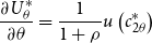
 \begin{equation} \frac{\partial \widehat{U}_{\theta }^{\ast }}{\partial \theta }=\frac{1}{1+\rho }u\left ( \widehat{c}_{2\theta }^{\ast }\right ), \end{equation}
can be regarded as the marginal benefit of longevity (MBL), measured in utility level, before the PA plan is introduced. When $\theta$
increases a little, a buyer has a higher chance of surviving to Period 2. Thus, the buyer has a higher chance of consuming
$\theta$
increases a little, a buyer has a higher chance of surviving to Period 2. Thus, the buyer has a higher chance of consuming $\widehat{c}_{2\theta }^{\ast }$
and thereby obtains the benefit of
$\widehat{c}_{2\theta }^{\ast }$
and thereby obtains the benefit of $u ( \widehat{c}_{2\theta }^{\ast } )$
. The RHS term in (36) represents this benefit, which is discounted back to Period 1. Similarly,
$u ( \widehat{c}_{2\theta }^{\ast } )$
. The RHS term in (36) represents this benefit, which is discounted back to Period 1. Similarly,
 \begin{equation} \frac{\partial U_{\theta }^{\ast }}{\partial \theta }=\frac{1}{1+\rho }u\left ( c_{2\theta }^{\ast }\right ) \end{equation}
captures the MBL after the PA plan is introduced. Combining them leads to (35), which is the difference of the MBL before and after the PA plan is introduced.
Since $u^{^{\prime }} (. ) > 0$
, whether
$u^{^{\prime }} (. ) > 0$
, whether $U_{\theta }^{\ast }-\widehat{U}_{\theta }^{\ast }$
is increasing or decreasing in
$U_{\theta }^{\ast }-\widehat{U}_{\theta }^{\ast }$
is increasing or decreasing in $\theta$
depends on the difference between
$\theta$
depends on the difference between $c_{2\theta }^{\ast }$
and
$c_{2\theta }^{\ast }$
and $\widehat{c}_{2\theta }^{\ast }$
. In subsequent analysis, we will use the gap between
$\widehat{c}_{2\theta }^{\ast }$
. In subsequent analysis, we will use the gap between $c_{2\theta }^{\ast }$
and
$c_{2\theta }^{\ast }$
and $\widehat{c}_{2\theta }^{\ast }$
to examine whether
$\widehat{c}_{2\theta }^{\ast }$
to examine whether $U_{\theta }^{\ast }-\widehat{U}_{\theta }^{\ast }$
is increasing or decreasing in survival probability (
$U_{\theta }^{\ast }-\widehat{U}_{\theta }^{\ast }$
is increasing or decreasing in survival probability ( $\theta$
) for different intervals of
$\theta$
) for different intervals of $\theta$
.
$\theta$
.
5.1 Effects under a VPA with ceiling plan
We consider the VPAc plan with the not-too-high ceiling condition (21). We first obtain a useful result in Lemma 2. The proof is given in the Online Appendix.
Lemma 2. If ( 21 ) holds, then
 \begin{equation} U_{\overline{\theta }}^{\ast }-\widehat{U}_{\overline{\theta }}^{\ast }< 0. \end{equation}
The intuition of Lemma 2 is as follows. When the VPAc plan is introduced, the retirees benefit from the higher level of PA payout $G^{\ast }$
(the severity reduction effect), but they can at most enjoy this benefit up to
$G^{\ast }$
(the severity reduction effect), but they can at most enjoy this benefit up to $m$
units of PA purchase. On the other hand, retirees who are very healthy and have residual demand for the private annuity suffer from the lower level of private annuity payout
$m$
units of PA purchase. On the other hand, retirees who are very healthy and have residual demand for the private annuity suffer from the lower level of private annuity payout $V^{\ast }$
(the private market distortion effect). Lemma 2 shows that when
$V^{\ast }$
(the private market distortion effect). Lemma 2 shows that when $m$
is set according to condition (21), the loss from the private market distortion effect for the healthiest retirees (with
$m$
is set according to condition (21), the loss from the private market distortion effect for the healthiest retirees (with $\theta =\overline{\theta }$
) dominates the benefit from the severity reduction effect. As a result, (38) holds and the healthiest annuity buyers are adversely affected by the introduction of the VPAc plan.
$\theta =\overline{\theta }$
) dominates the benefit from the severity reduction effect. As a result, (38) holds and the healthiest annuity buyers are adversely affected by the introduction of the VPAc plan.
With the help of Lemmas 1 and 2, we obtain the systematically different effects of introducing the VPAc plan on two categories of buyers, based on their survival probabilities ( $\theta$
).Footnote
23
The result is summarized in the following proposition.
$\theta$
).Footnote
23
The result is summarized in the following proposition.
Proposition 3.
When the government introduces a VPAc plan such that parameter $m$
satisfies (
21
), the VPAc plan systematically separates annuity buyers in two categories according to the change in utility level: (a) an increase in a buyer’s utility level for the poor health group; and (b) a decrease in a buyer’s utility level for the good health group.
$m$
satisfies (
21
), the VPAc plan systematically separates annuity buyers in two categories according to the change in utility level: (a) an increase in a buyer’s utility level for the poor health group; and (b) a decrease in a buyer’s utility level for the good health group.
Proof. See Appendix B.
The policy implications of Proposition 3, together with those of Proposition 4 regarding the MPAf plan in Section 5.2, will be discussed in Section 5.3.
5.2 Effects under a MPA with flexibility plan
We now consider the MPAf plan. The following lemma is useful for analyzing the utility effects under this plan. The proof is given in the Online Appendix.
Lemma 3. If
 \begin{equation} f> \underline{f}, \end{equation}
where $\underline{f}$
is the larger root to
$\underline{f}$
is the larger root to
 \begin{equation} U_{\underline{\theta }}\left ( \underline{f}\right ) =u\left ( w-\underline{f}\right ) +\frac{\underline{\theta }}{1+\rho }u\left ( G^{\ast }\underline{f}\right ) =\widehat{U}_{\underline{\theta }}^{\ast }, \end{equation}
with $G^{\ast }$
given by (
30
) and
$G^{\ast }$
given by (
30
) and $\widehat{U}_{\underline{\theta }}^{\ast }=u\left ( w-\widehat{v}_{\underline{\theta }}^{\ast }\right ) +\frac{\underline{\theta }}{1+\rho }u\left ( \widehat{V}^{\ast }\widehat{v}_{\underline{\theta }}^{\ast }\right )$
, then
$\widehat{U}_{\underline{\theta }}^{\ast }=u\left ( w-\widehat{v}_{\underline{\theta }}^{\ast }\right ) +\frac{\underline{\theta }}{1+\rho }u\left ( \widehat{V}^{\ast }\widehat{v}_{\underline{\theta }}^{\ast }\right )$
, then
 \begin{equation} U_{\underline{\theta }}^{\ast }-\widehat{U}_{\underline{\theta }}^{\ast }< 0. \end{equation}
If
 \begin{equation} \widehat{\nu }_{\underline{\theta }}^{\ast }\leq f\leq \underline{f}, \end{equation}
then ( 41 ) does not hold.
Under the MPAf plan, retirees with poor health (such as those with $\theta < \theta _{fo}$
) benefit from the higher PA payout (
$\theta < \theta _{fo}$
) benefit from the higher PA payout ( $G^{\ast }$
) but are adversely affected by the restriction to buy the mandated level (
$G^{\ast }$
) but are adversely affected by the restriction to buy the mandated level ( $f$
) of PA purchase. Lemma 3 shows that if the floor is set at a not-too-low level (i.e. (39) holds), then for retirees with the lowest survival probability (
$f$
) of PA purchase. Lemma 3 shows that if the floor is set at a not-too-low level (i.e. (39) holds), then for retirees with the lowest survival probability ( $\underline{\theta }$
), the mandated floor level deviates quite substantially from their annuity demand (as measured by
$\underline{\theta }$
), the mandated floor level deviates quite substantially from their annuity demand (as measured by $\widehat{\nu }_{\underline{\theta }}^{\ast }$
before the PA plan is introduced). As a result, (41) holds and annuity buyers with the lowest survival probability are adversely adversely by the introduction of the MPAf plan, because the loss from the restriction to buy the mandated PA level dominates the benefit from the higher PA payout.
$\widehat{\nu }_{\underline{\theta }}^{\ast }$
before the PA plan is introduced). As a result, (41) holds and annuity buyers with the lowest survival probability are adversely adversely by the introduction of the MPAf plan, because the loss from the restriction to buy the mandated PA level dominates the benefit from the higher PA payout.
We now focus on the more interesting case that the not-too-low floor condition (39) holds.Footnote
24
The following proposition summarizes the results that introducing the MPAf plan has systematically different effects on three categories of buyers, based on their survival probabilities ( $\theta$
).
$\theta$
).
Proposition 4.
When the government introduces a MPAf plan such that parameter $m$
satisfies (
21
) and parameter
$m$
satisfies (
21
) and parameter $f$
satisfies (
39
), the MPAf plan systematically separates annuity buyers in three categories according to the change in utility level: (a) a decrease in a buyer’s utility level for the poor health group; (b) an increase in a buyer’s utility level for the group with average health; and (c) a decrease in a buyer’s utility level for the good health group.
$f$
satisfies (
39
), the MPAf plan systematically separates annuity buyers in three categories according to the change in utility level: (a) a decrease in a buyer’s utility level for the poor health group; (b) an increase in a buyer’s utility level for the group with average health; and (c) a decrease in a buyer’s utility level for the good health group.
The proof of Proposition 4 is given in the Online Appendix. Most parts of the proof are similar to those of Proposition 3.
Propositions 3 and 4 appear to be quite different, with one threshold for the VPAc plan in Proposition 3 but two thresholds for the MPAf plan in Proposition 4 when (39) holds.Footnote
25
There is actually a similarity between Propositions 3 and 4 in that the utility difference ( $U_{\theta }^{\ast }-\widehat{U}_{\theta }^{\ast }$
) for either the VPAc or MPAf plan is first increasing in
$U_{\theta }^{\ast }-\widehat{U}_{\theta }^{\ast }$
) for either the VPAc or MPAf plan is first increasing in $\theta$
and then decreasing in
$\theta$
and then decreasing in $\theta$
after reaching a maximum. As a result, there is a single peak in the
$\theta$
after reaching a maximum. As a result, there is a single peak in the $U_{\theta }^{\ast }-\widehat{U}_{\theta }^{\ast }$
function for either PA plan. The above framework also helps understand the main factor leading to Proposition 4. When
$U_{\theta }^{\ast }-\widehat{U}_{\theta }^{\ast }$
function for either PA plan. The above framework also helps understand the main factor leading to Proposition 4. When $f$
is set according to condition (39), the floor has a strong effect in restricting the PA purchases by retirees of poor health. Thus, the distortion caused by the mandated floor level dominates the severity reduction effect, leading to (41) for the least healthy buyers. Together with the single peak property of the
$f$
is set according to condition (39), the floor has a strong effect in restricting the PA purchases by retirees of poor health. Thus, the distortion caused by the mandated floor level dominates the severity reduction effect, leading to (41) for the least healthy buyers. Together with the single peak property of the $U_{\theta }^{\ast }-\widehat{U}_{\theta }^{\ast }$
function, it can be shown (in the Online Appendix) that there are three categories of buyers.Footnote
26
$U_{\theta }^{\ast }-\widehat{U}_{\theta }^{\ast }$
function, it can be shown (in the Online Appendix) that there are three categories of buyers.Footnote
26
5.3 Which PA plan to adopt: Voluntary or mandatory?
Our analysis provides some guidance regarding which PA plan the government wants to adopt. Whatever the MPAf or VPAc plan is adopted, the average health group benefits but the good health group is adversely affected.Footnote 27 The intuition is that the annuity buyers with average health purchase some, but not excessive, amount of annuity before the PA plan is introduced. Thus, when the PA plan is introduced, they benefit from the higher PA payout but their optimal choices of annuity quantity are not severely distorted by the restriction of either plan. On the other hand, the negative private market distortion effect is more important to the good health group, leading to a drop in utility level. For the poor health group, the change in utility level depends on which PA plan is adopted. In particular, retirees with poor health are adversely affected in the MPAf plan with condition (39) because the minimum mandated level of annuity purchase differs substantially from their desired levels in the absence of the plan, but benefit from the VPAc plan because there is no floor restriction that would otherwise distort the amount of their PA purchase.
While the government’s ultimate decision to adopt a particular PA plan depends on many economic and political factors, our analysis based on a simple two-period model brings out some important factors (the severity reduction and private market distortion effects) clearly and shows how the two existing PA plans have systematically different utility effects on the retirees with different health characteristics.Footnote 28
6. Conclusion
There are two major types of observed PA plans: voluntary plans with ceiling restriction and mandatory plans with some flexibility. We study the similarities and differences of these PA plans. In both plans, the restrictive element due to the quantity restriction leads to a positive effect that mitigates the severity of adverse selection in the PA sector, but it also causes a negative effect that amplifies the distortion in the private market. On the other hand, the flexibility component performs the moderating function that reduces the magnitude of each of these two effects. Our results suggest that the consequence of offering the PA plan is a compromise of its positive severity reduction effect on public annuities and its negative private market distortion effect on private annuities.
Our study provides guidance to the economies planning to introduce the PA plan. First, the introduction of the PA plan, either voluntary or mandatory, leads to a two-tier annuity market. Retirees first buy the PA because it offers a higher payout. The private annuity market still has a role to play, as some buyers have excessive demands that are unfulfilled by the restriction of the PA plan and purchase annuities from the private market. Second, the introduction of a PA plan, either mandatory or voluntary, divides the population into different groups based on whether they benefit or are adversely affected in the newly introduced PA plan. Our analysis suggests that the retirees with average survival probability benefit from the PA plan, whereas the retirees with a high level of survival probability are adversely affected. The effects on the retirees with a low level of survival probability depend on which PA plan is offered; in particular, they are adversely affected in the MPAf plan when the floor parameter ( $f$
) is set at a not-too-low level. Before deciding to introduce a particular PA plan to the retirees, the government should consider seriously the effects on different groups of retirees who benefit from or are adversely affected by the plan.
$f$
) is set at a not-too-low level. Before deciding to introduce a particular PA plan to the retirees, the government should consider seriously the effects on different groups of retirees who benefit from or are adversely affected by the plan.
Supplementary material
To view supplementary material for this article, please visit https://doi.org/10.1017/S1365100523000093.
Appendix
We prove Propositions 1 and 3 in Appendices A and B, respectively.
Appendix A: Proof of Proposition 1
We focus on the MPAf plan in this Appendix. The proof for the simpler VPAc plan is similar and is given in the Online Appendix.
(A) Under the MPAf plan with (27) and (28), define the function
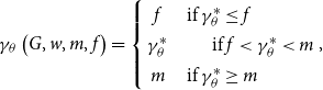 \begin{equation} \gamma _{\theta }\left ( G,w,m,f\right ) =\left \{ \begin{array}{c@{\quad}l} f & \text{if }\gamma _{\theta }^{\ast }\leq f \\ \gamma _{\theta }^{\ast } & \,\,\,\,\,\,\,\,\text{ if }f< \gamma _{\theta }^{\ast }< m \\ m & \text{if }\gamma _{\theta }^{\ast }\geq m\end{array}\right .\!, \end{equation}
where the optimal PA purchase $\gamma _{\theta }^{\ast }$
is defined in (23). Based on (A1), define the function
$\gamma _{\theta }^{\ast }$
is defined in (23). Based on (A1), define the function
 \begin{equation} J\left ( G,w,m,f\right ) =\frac{\left ( 1+r\right ) \int _{\underline{\theta }}^{\overline{\theta }}\gamma _{\theta }\left ( G,w,m,f\right ) dF(\theta )}{\int _{\underline{\theta }}^{\overline{\theta }}\theta \gamma _{\theta }\left ( G,w,m,f\right ) dF(\theta )}. \end{equation}
Based on (30) and (A2), the equilibrium payout ( $G^{\ast }$
) is defined byFootnote
29
$G^{\ast }$
) is defined byFootnote
29
 \begin{equation} J\left ( G^{\ast },w,m,f\right ) =\frac{\left ( 1+r\right ) \int _{\underline{\theta }}^{\overline{\theta }}\gamma _{\theta }\left ( G^{\ast },w,m,f\right ) dF(\theta )}{\int _{\underline{\theta }}^{\overline{\theta }}\theta \gamma _{\theta }\left ( G^{\ast },w,m,f\right ) dF(\theta )}=G^{\ast }. \end{equation}
We study $J ( G,w,m,f )$
as a function of
$J ( G,w,m,f )$
as a function of $G$
when
$G$
when $G\in \left [ \widehat{V}^{\ast },\frac{1+r}{E\left ( \theta \right ) }\right ]$
and look for the intersection of this function and the 45-degree line, as shown in Panel A of Figure A1. First, consider
$G\in \left [ \widehat{V}^{\ast },\frac{1+r}{E\left ( \theta \right ) }\right ]$
and look for the intersection of this function and the 45-degree line, as shown in Panel A of Figure A1. First, consider $J ( G,w,m,f )$
at the beginning point
$J ( G,w,m,f )$
at the beginning point $G=\widehat{V}^{\ast }$
. It can be shown from (6), (23), and (A1) that
$G=\widehat{V}^{\ast }$
. It can be shown from (6), (23), and (A1) that $\frac{\gamma _{\theta }\left ( \widehat{V}^{\ast },w,m,f\right ) }{\widehat{\nu }_{\theta }^{\ast }}$
(i) is larger than 1 and strictly decreasing for low value of
$\frac{\gamma _{\theta }\left ( \widehat{V}^{\ast },w,m,f\right ) }{\widehat{\nu }_{\theta }^{\ast }}$
(i) is larger than 1 and strictly decreasing for low value of $\theta$
such that
$\theta$
such that $\widehat{\nu }_{\theta }^{\ast }< f$
, (ii) is less than 1 and strictly decreasing for high value of
$\widehat{\nu }_{\theta }^{\ast }< f$
, (ii) is less than 1 and strictly decreasing for high value of $\theta$
such that
$\theta$
such that $\widehat{\nu }_{\theta }^{\ast }> m$
, or (iii) equals to 1 for the intermediate values of
$\widehat{\nu }_{\theta }^{\ast }> m$
, or (iii) equals to 1 for the intermediate values of $\theta$
. As a result, the function
$\theta$
. As a result, the function $\frac{\gamma _{\theta }\left ( \widehat{V}^{\ast },w,m,f\right ) }{\widehat{\nu }_{\theta }^{\ast }}$
is weakly decreasing for all
$\frac{\gamma _{\theta }\left ( \widehat{V}^{\ast },w,m,f\right ) }{\widehat{\nu }_{\theta }^{\ast }}$
is weakly decreasing for all $\theta \in [ \underline{\theta },\overline{\theta } ]$
, with a strictly decreasing part over some interval. Thus, the Chebyshev’s Sum
$\theta \in [ \underline{\theta },\overline{\theta } ]$
, with a strictly decreasing part over some interval. Thus, the Chebyshev’s Sum
 \begin{equation} \int _{\underline{\theta }}^{\overline{\theta }}\int _{\underline{\theta }}^{\overline{\theta }}\left ( x-y\right ) \left [ \frac{\gamma _{x}\left ( \widehat{V}^{\ast },w,m,f\right ) }{\widehat{\nu }_{x}^{\ast }}-\frac{\gamma _{y}\left ( \widehat{V}^{\ast },w,m,f\right ) }{\widehat{\nu }_{y}^{\ast }}\right ] \widehat{\nu }_{x}^{\ast }\widehat{\nu }_{y}^{\ast }dF(x)dF(y) \end{equation}
is negative, where $x$
and
$x$
and $y$
are two arbitrary indexes. This leads toFootnote
30
$y$
are two arbitrary indexes. This leads toFootnote
30

Figure A1. The determination of equilibrium annuity payouts.
 \begin{equation} J\left ( \widehat{V}^{\ast },w,m,f\right ) =\frac{\left ( 1+r\right ) \int _{\underline{\theta }}^{\overline{\theta }}\gamma _{\theta }\left ( \widehat{V}^{\ast },w,m,f\right ) dF(\theta )}{\int _{\underline{\theta }}^{\overline{\theta }}\theta \gamma _{\theta }\left ( \widehat{V}^{\ast },w,m,f\right ) dF(\theta )}> \frac{\left ( 1+r\right ) \int _{\underline{\theta }}^{\overline{\theta }}\widehat{\nu }_{\theta }^{\ast }dF(\theta )}{\int _{\underline{\theta }}^{\overline{\theta }}\theta \widehat{\nu }_{\theta }^{\ast }dF(\theta )}=\widehat{V}^{\ast }. \end{equation}
Second, consider $J ( G,w,m,f )$
at the end point
$J ( G,w,m,f )$
at the end point $G=\frac{1+r}{E\left ( \theta \right ) }$
. It is easy to show that
$G=\frac{1+r}{E\left ( \theta \right ) }$
. It is easy to show that
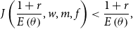 \begin{equation} J\left ( \frac{1+r}{E\left ( \theta \right ) },w,m,f\right ) < \frac{1+r}{E\left ( \theta \right ) }, \end{equation}
because when adverse selection is present, the PA payout based on the retirees’ behavior (the LHS term) is always lower than the (hypothetical) payout based on the average survival probability of the retirees (the RHS term).
The $J ( G,w,m,f )$
function is above the 45-degree line at
$J ( G,w,m,f )$
function is above the 45-degree line at $G=\widehat{V}^{\ast }$
, and below it at
$G=\widehat{V}^{\ast }$
, and below it at $G=\frac{1+r}{E\left ( \theta \right ) }$
. Together with the continuity of the
$G=\frac{1+r}{E\left ( \theta \right ) }$
. Together with the continuity of the $J ( G,w,m,f )$
function, we conclude that there exists an equilibrium value of
$J ( G,w,m,f )$
function, we conclude that there exists an equilibrium value of $G^{\ast }$
which is larger than
$G^{\ast }$
which is larger than $\widehat{V}^{\ast }$
. (See Panel A of Figure A1.) This proves part (a) of Proposition 1.
$\widehat{V}^{\ast }$
. (See Panel A of Figure A1.) This proves part (a) of Proposition 1.
(B) Based on the optimal private annuity purchase ( $\nu _{\theta }^{\ast }$
) in (15) with
$\nu _{\theta }^{\ast }$
) in (15) with $G=G^{\ast }$
, define the function
$G=G^{\ast }$
, define the function
 \begin{equation} \nu _{\theta }\left ( V,w,m\right ) =\max \left \{ 0,\nu _{\theta }^{\ast }\right \}, \end{equation}
where other parameter values (including $G^{\ast }$
) are unchanged. Based on (A7), we define the function
$G^{\ast }$
) are unchanged. Based on (A7), we define the function
 \begin{equation} K\left ( V,w,m\right ) =\frac{\left ( 1+r\right ) \int _{\underline{\theta }}^{\overline{\theta }}\nu _{\theta }\left ( V,w,m\right ) dF(\theta )}{\int _{\underline{\theta }}^{\overline{\theta }}\theta \nu _{\theta }\left ( V,w,m\right ) dF(\theta )}. \end{equation}
Based on (18) and (A8), the equilibrium private annuity payout ( $V^{\ast }$
) in the presence of the PA plan is defined by
$V^{\ast }$
) in the presence of the PA plan is defined by
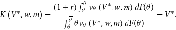 \begin{equation} K\left ( V^{\ast },w,m\right ) =\frac{\left ( 1+r\right ) \int _{\underline{\theta }}^{\overline{\theta }}\nu _{\theta }\left ( V^{\ast },w,m\right ) dF(\theta )}{\int _{\underline{\theta }}^{\overline{\theta }}\theta \nu _{\theta }\left ( V^{\ast },w,m\right ) dF(\theta )}=V^{\ast }. \end{equation}
We study $K ( V,w,m )$
as a function of
$K ( V,w,m )$
as a function of $V$
when
$V$
when $V\in \left [ \frac{1+r}{\overline{\theta }},\widehat{V}^{\ast }\right ]$
and look for the intersection of this function and the 45-degree line, as shown in Panel B of Figure A1. First, consider
$V\in \left [ \frac{1+r}{\overline{\theta }},\widehat{V}^{\ast }\right ]$
and look for the intersection of this function and the 45-degree line, as shown in Panel B of Figure A1. First, consider $K ( V,w,m )$
when
$K ( V,w,m )$
when $V=\frac{1+r}{\overline{\theta }}$
. It is easy to show that
$V=\frac{1+r}{\overline{\theta }}$
. It is easy to show that
 \begin{equation} K\left ( \frac{1+r}{\overline{\theta }},w,m\right ) > \frac{1+r}{\overline{\theta }}, \end{equation}
because there are some buyers who have residual demand (after buying the PA) even when the annuity payout is as low as $\frac{1+r}{\overline{\theta }}$
. As long as some buyers demand the private annuity, (A10) holds.
$\frac{1+r}{\overline{\theta }}$
. As long as some buyers demand the private annuity, (A10) holds.
Second, consider $K ( V,w,m )$
when
$K ( V,w,m )$
when $V=\widehat{V}^{\ast }$
. Our objective is to compare
$V=\widehat{V}^{\ast }$
. Our objective is to compare $\nu _{\theta } ( \widehat{V}^{\ast },w,m )$
with
$\nu _{\theta } ( \widehat{V}^{\ast },w,m )$
with $\widehat{\nu }_{\theta }^{\ast }\equiv \nu _{\theta } ( \widehat{V}^{\ast },w,0 )$
. A direct comparison turns out to be difficult, and we rely on an intermediate term:
$\widehat{\nu }_{\theta }^{\ast }\equiv \nu _{\theta } ( \widehat{V}^{\ast },w,0 )$
. A direct comparison turns out to be difficult, and we rely on an intermediate term: $\nu _{\theta } ( \widehat{V}^{\ast },w^{h},0 )$
, as follows.
$\nu _{\theta } ( \widehat{V}^{\ast },w^{h},0 )$
, as follows.
For a retiree whose desired annuity choice is not constrained by the PA plan (i.e. it is an interior solution), we consider the hypothetical environment in which she is given extra resources up to the new wealth level of $w^{h}$
but is only allowed to buy the private annuity with payout
$w^{h}$
but is only allowed to buy the private annuity with payout $\widehat{V}^{\ast }$
. We want to find the level of
$\widehat{V}^{\ast }$
. We want to find the level of $w^{h}$
such that the individual’s optimal choices of
$w^{h}$
such that the individual’s optimal choices of $c_{1\theta }$
and
$c_{1\theta }$
and $c_{2\theta }$
will be the same (and thus the first-order condition is the same) as those chosen at her original level of wealth (
$c_{2\theta }$
will be the same (and thus the first-order condition is the same) as those chosen at her original level of wealth ( $w$
) when both PA (with the equilibrium payout
$w$
) when both PA (with the equilibrium payout $G^{\ast }$
) and private annuity (with the hypothetical payout
$G^{\ast }$
) and private annuity (with the hypothetical payout $\widehat{V}^{\ast }$
) are available. Since
$\widehat{V}^{\ast }$
) are available. Since $\gamma _{\theta }^{\ast }=m$
for any retiree in this group, we can use (3), (4), (10), and (11) to show that the optimal annuity choices are related by
$\gamma _{\theta }^{\ast }=m$
for any retiree in this group, we can use (3), (4), (10), and (11) to show that the optimal annuity choices are related by
 \begin{equation} \nu _{\theta }\left ( \widehat{V}^{\ast },w^{h},0\right ) =\nu _{\theta }\left ( \widehat{V}^{\ast },w,m\right ) +\frac{G^{\ast }}{\widehat{V}^{\ast }}m, \end{equation}
and the actual and hypothetical levels of wealth are related by
 \begin{equation} w^{h}=w+\left ( \frac{G^{\ast }}{\widehat{V}^{\ast }}-1\right ) m, \end{equation}
where $\nu _{\theta } ( \widehat{V}^{\ast },w,m )$
and
$\nu _{\theta } ( \widehat{V}^{\ast },w,m )$
and $\nu _{\theta } ( \widehat{V}^{\ast },w^{h},0 )$
are determined according to (A7).
$\nu _{\theta } ( \widehat{V}^{\ast },w^{h},0 )$
are determined according to (A7).
We now examine $\frac{\nu _{\theta }\left ( \widehat{V}^{\ast },w^{h},0\right ) }{\nu _{\theta }\left ( \widehat{V}^{\ast },w,0\right ) }$
, where
$\frac{\nu _{\theta }\left ( \widehat{V}^{\ast },w^{h},0\right ) }{\nu _{\theta }\left ( \widehat{V}^{\ast },w,0\right ) }$
, where $\nu _{\theta } ( \widehat{V}^{\ast },w^{h},0 )$
and
$\nu _{\theta } ( \widehat{V}^{\ast },w^{h},0 )$
and $\nu _{\theta } ( \widehat{V}^{\ast },w,0 )$
are the optimal choices in two similar environments which have the same annuity payout (
$\nu _{\theta } ( \widehat{V}^{\ast },w,0 )$
are the optimal choices in two similar environments which have the same annuity payout ( $\widehat{V}^{\ast }$
) but different wealth levels. When the utility function
$\widehat{V}^{\ast }$
) but different wealth levels. When the utility function $U ( c_{1\theta },c_{2\theta };\,\ \theta )$
in (1) is homothetic, condition (2) holds, leading to the result that the wealth elasticity of consumption at either period is unity. Together with (4), the share of annuity purchase to wealth is constant. Putting
$U ( c_{1\theta },c_{2\theta };\,\ \theta )$
in (1) is homothetic, condition (2) holds, leading to the result that the wealth elasticity of consumption at either period is unity. Together with (4), the share of annuity purchase to wealth is constant. Putting $t=\frac{w^{h}}{w}$
in (2) where
$t=\frac{w^{h}}{w}$
in (2) where $w^{h}$
is defined in (A12), it can be shown that
$w^{h}$
is defined in (A12), it can be shown that
 \begin{equation} \frac{\nu _{\theta }\left ( \widehat{V}^{\ast },w^{h},0\right ) }{\nu _{\theta }\left ( \widehat{V}^{\ast },w,0\right ) }=\frac{w^{h}}{w}=1+\left ( \frac{G^{\ast }}{\widehat{V}^{\ast }}-1\right ) \frac{m}{w} \end{equation}
does not depend on $\theta$
.
$\theta$
.
Combining (A11) and (A13), it can be shown that
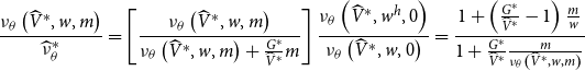 \begin{equation} \frac{\nu _{\theta }\left ( \widehat{V}^{\ast },w,m\right ) }{\widehat{\nu }_{\theta }^{\ast }}=\left [ \frac{\nu _{\theta }\left ( \widehat{V}^{\ast },w,m\right ) }{\nu _{\theta }\left ( \widehat{V}^{\ast },w,m\right ) +\frac{G^{\ast }}{\widehat{V}^{\ast }}m}\right ] \frac{\nu _{\theta }\left ( \widehat{V}^{\ast },w^{h},0\right ) }{\nu _{\theta }\left ( \widehat{V}^{\ast },w,0\right ) }=\frac{1+\left ( \frac{G^{\ast }}{\widehat{V}^{\ast }}-1\right ) \frac{m}{w}}{1+\frac{G^{\ast }}{\widehat{V}^{\ast }}\frac{m}{\nu _{\theta }\left ( \widehat{V}^{\ast },w,m\right ) }} \end{equation}
is strictly increasing in $\theta$
for
$\theta$
for $\theta > \frac{\left ( 1+\rho \right ) u^{\prime }\left ( w-m\right ) }{\widehat{V}^{\ast }u^{\prime }\left ( G^{\ast }m\right ) }$
, because
$\theta > \frac{\left ( 1+\rho \right ) u^{\prime }\left ( w-m\right ) }{\widehat{V}^{\ast }u^{\prime }\left ( G^{\ast }m\right ) }$
, because $\nu _{\theta } ( \widehat{V}^{\ast },w,m )$
is increasing in
$\nu _{\theta } ( \widehat{V}^{\ast },w,m )$
is increasing in $\theta$
for interior solutions. Together with
$\theta$
for interior solutions. Together with $\frac{\nu _{\theta }\left ( \widehat{V}^{\ast },w,m\right ) }{\widehat{\nu }_{\theta }^{\ast }}=0$
for
$\frac{\nu _{\theta }\left ( \widehat{V}^{\ast },w,m\right ) }{\widehat{\nu }_{\theta }^{\ast }}=0$
for $\theta \leq \frac{\left ( 1+\rho \right ) u^{\prime }\left ( w-m\right ) }{\widehat{V}^{\ast }u^{\prime }\left ( G^{\ast }m\right ) }$
, we conclude that the Chebyshev’s Sum
$\theta \leq \frac{\left ( 1+\rho \right ) u^{\prime }\left ( w-m\right ) }{\widehat{V}^{\ast }u^{\prime }\left ( G^{\ast }m\right ) }$
, we conclude that the Chebyshev’s Sum
 \begin{equation} \int _{\underline{\theta }}^{\overline{\theta }}\int _{\underline{\theta }}^{\overline{\theta }}\left ( x-y\right ) \left [ \frac{\nu _{x}\left ( \widehat{V}^{\ast },w,m\right ) }{\widehat{\nu }_{x}^{\ast }}-\frac{\nu _{y}\left ( \widehat{V}^{\ast },w,m\right ) }{\widehat{\nu }_{y}^{\ast }}\right ] \widehat{\nu }_{x}^{\ast }\widehat{\nu }_{y}^{\ast }dF(x)dF(y) \end{equation}
is positive, leading toFootnote 31
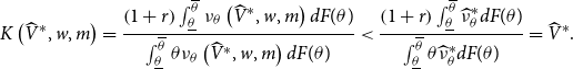 \begin{equation} K\left ( \widehat{V}^{\ast },w,m\right ) =\frac{\left ( 1+r\right ) \int _{\underline{\theta }}^{\overline{\theta }}\nu _{\theta }\left ( \widehat{V}^{\ast },w,m\right ) dF(\theta )}{\int _{\underline{\theta }}^{\overline{\theta }}\theta \nu _{\theta }\left ( \widehat{V}^{\ast },w,m\right ) dF(\theta )}< \frac{\left ( 1+r\right ) \int _{\underline{\theta }}^{\overline{\theta }}\widehat{\nu }_{\theta }^{\ast }dF(\theta )}{\int _{\underline{\theta }}^{\overline{\theta }}\theta \widehat{\nu }_{\theta }^{\ast }dF(\theta )}=\widehat{V}^{\ast }. \end{equation}
Combining (A9), (A10), (A16) and the continuity of the $K ( V,w,m )$
function, we conclude that there exists an equilibrium value of
$K ( V,w,m )$
function, we conclude that there exists an equilibrium value of $V^{\ast }$
which is smaller than
$V^{\ast }$
which is smaller than $\widehat{V}^{\ast }$
. This proves part (b) of Proposition 1.
$\widehat{V}^{\ast }$
. This proves part (b) of Proposition 1.
Appendix B: Proof of Proposition 3
For the VPAc plan, it is convenient to label $\theta \in \lbrack \underline{\theta },\theta _{om})$
as Region A,
$\theta \in \lbrack \underline{\theta },\theta _{om})$
as Region A, $\theta \in \lbrack \theta _{om},\theta _{mb})$
as Region B, and
$\theta \in \lbrack \theta _{om},\theta _{mb})$
as Region B, and $\theta \in \lbrack \theta _{mb},\overline{\theta }]$
as Region C (See Figure A2.)
$\theta \in \lbrack \theta _{mb},\overline{\theta }]$
as Region C (See Figure A2.)
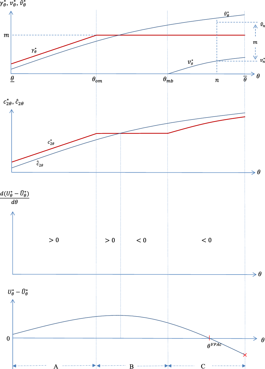
Figure A2. Utility comparison under the VPAc plan.
The following lemma is useful for the analysis regarding Region C. The proof is given in the Online Appendix.
Lemma A1.
In Region C, $c_{2\theta }^{\ast }$
and
$c_{2\theta }^{\ast }$
and $\widehat{c}_{2\theta }^{\ast }$
either intersect once or do not intersect.
$\widehat{c}_{2\theta }^{\ast }$
either intersect once or do not intersect.
In the following, we first prove Lemma 1. We then use this result, as well as Lemmas 2 and A1, to prove Proposition 3.
B.1. Proof of Lemma 1
Differentiating (5) with respect to $\theta$
, evaluated at the optimal choices, and using the first-order condition (6), we obtain (36).
$\theta$
, evaluated at the optimal choices, and using the first-order condition (6), we obtain (36).
The proof for the economy after the introduction of the VPAc plan is similar but slightly more tedious. Differentiating (1) with respect to $\theta$
, evaluated at the optimal choices, and using (23), we obtain (37) in Region A. Similarly, differentiating (1) with respect to
$\theta$
, evaluated at the optimal choices, and using (23), we obtain (37) in Region A. Similarly, differentiating (1) with respect to $\theta$
, evaluated at the optimal choices, and using (15), we obtain (37) in Region C. The analysis for Region B is simpler because the optimal choice of
$\theta$
, evaluated at the optimal choices, and using (15), we obtain (37) in Region C. The analysis for Region B is simpler because the optimal choice of $c_{1\theta }^{\ast }$
is the same for all buyers in this region. As a result, (37) holds.
$c_{1\theta }^{\ast }$
is the same for all buyers in this region. As a result, (37) holds.
B.2. Proof of Proposition 3
First, we focus on Region A. The choices $\widehat{c}_{1\theta }^{\ast }$
and
$\widehat{c}_{1\theta }^{\ast }$
and $\widehat{c}_{2\theta }^{\ast }$
are feasible under the VPAc plan because of (31), but they are not optimal since they do not satisfy the first-order condition (23). Moreover, the combination of
$\widehat{c}_{2\theta }^{\ast }$
are feasible under the VPAc plan because of (31), but they are not optimal since they do not satisfy the first-order condition (23). Moreover, the combination of $c_{1\theta }^{\ast }\leq \widehat{c}_{1\theta }^{\ast }$
and
$c_{1\theta }^{\ast }\leq \widehat{c}_{1\theta }^{\ast }$
and $c_{2\theta }^{\ast }\leq \widehat{c}_{2\theta }^{\ast }$
is inconsistent with the two lifetime budget constraints (with and without the PA plan),Footnote
32
and the combination of
$c_{2\theta }^{\ast }\leq \widehat{c}_{2\theta }^{\ast }$
is inconsistent with the two lifetime budget constraints (with and without the PA plan),Footnote
32
and the combination of $c_{1\theta }^{\ast }> \widehat{c}_{1\theta }^{\ast }$
and
$c_{1\theta }^{\ast }> \widehat{c}_{1\theta }^{\ast }$
and $c_{2\theta }^{\ast }\leq \widehat{c}_{2\theta }^{\ast }$
is inconsistent with the two relevant first-order conditions (6) and (23).Footnote
33
Combining the above results, we conclude that
$c_{2\theta }^{\ast }\leq \widehat{c}_{2\theta }^{\ast }$
is inconsistent with the two relevant first-order conditions (6) and (23).Footnote
33
Combining the above results, we conclude that $c_{2\theta }^{\ast }> \widehat{c}_{2\theta }^{\ast }$
and
$c_{2\theta }^{\ast }> \widehat{c}_{2\theta }^{\ast }$
and $U_{\theta }^{\ast }> \widehat{U}_{\theta }^{\ast }$
in Region A. This is Result 1.
$U_{\theta }^{\ast }> \widehat{U}_{\theta }^{\ast }$
in Region A. This is Result 1.
Applying Lemma 1, we conclude that $\frac{\partial \left ( U_{\theta }^{\ast }-\widehat{U}_{\theta }^{\ast }\right ) }{\partial \theta }> 0$
in Region A; thus,
$\frac{\partial \left ( U_{\theta }^{\ast }-\widehat{U}_{\theta }^{\ast }\right ) }{\partial \theta }> 0$
in Region A; thus, $U_{\theta }^{\ast }-\widehat{U}_{\theta }^{\ast }$
is increasing in this region. Combining it with
$U_{\theta }^{\ast }-\widehat{U}_{\theta }^{\ast }$
is increasing in this region. Combining it with $U_{\theta }^{\ast }> \widehat{U}_{\theta }^{\ast }$
in Region A, we conclude that
$U_{\theta }^{\ast }> \widehat{U}_{\theta }^{\ast }$
in Region A, we conclude that $U_{\theta }^{\ast }-\widehat{U}_{\theta }^{\ast }$
starts from a positive value when
$U_{\theta }^{\ast }-\widehat{U}_{\theta }^{\ast }$
starts from a positive value when $\theta =\underline{\theta }$
, and it increases and continues to be positive in Region A. This is Result 2.
$\theta =\underline{\theta }$
, and it increases and continues to be positive in Region A. This is Result 2.
Next, it is easy to see that $c_{2\theta }^{\ast }$
is constant and
$c_{2\theta }^{\ast }$
is constant and $\widehat{c}_{2\theta }^{\ast }$
is increasing in Region B. Together with Result 1, we conclude that there are two possible cases in Region B: (a)
$\widehat{c}_{2\theta }^{\ast }$
is increasing in Region B. Together with Result 1, we conclude that there are two possible cases in Region B: (a) $\widehat{c}_{2\theta }^{\ast }$
is increasing and passes the constant level of
$\widehat{c}_{2\theta }^{\ast }$
is increasing and passes the constant level of $c_{2\theta }^{\ast }$
once, and as a result,
$c_{2\theta }^{\ast }$
once, and as a result, $U_{\theta }^{\ast }-\widehat{U}_{\theta }^{\ast }$
is first increasing and then decreasing after reaching a maximum; or (b)
$U_{\theta }^{\ast }-\widehat{U}_{\theta }^{\ast }$
is first increasing and then decreasing after reaching a maximum; or (b) $\widehat{c}_{2\theta }^{\ast }$
is increasing but still below
$\widehat{c}_{2\theta }^{\ast }$
is increasing but still below $c_{2\theta }^{\ast }$
, and as a result,
$c_{2\theta }^{\ast }$
, and as a result, $U_{\theta }^{\ast }-\widehat{U}_{\theta }^{\ast }$
is increasing (and is always positive). Call them Case (a) and Case (b), respectively.
$U_{\theta }^{\ast }-\widehat{U}_{\theta }^{\ast }$
is increasing (and is always positive). Call them Case (a) and Case (b), respectively.
Regarding Region C, we show that the combination of $c_{1\overline{\theta }}^{\ast }< \widehat{c}_{1\overline{\theta }}^{\ast }$
and
$c_{1\overline{\theta }}^{\ast }< \widehat{c}_{1\overline{\theta }}^{\ast }$
and $c_{2\overline{\theta }}^{\ast }\geq \widehat{c}_{2\overline{\theta }}^{\ast }$
is inconsistent with (32) and the first-order conditions (6) and (15). On the other hand, the combination of
$c_{2\overline{\theta }}^{\ast }\geq \widehat{c}_{2\overline{\theta }}^{\ast }$
is inconsistent with (32) and the first-order conditions (6) and (15). On the other hand, the combination of $c_{1\overline{\theta }}^{\ast }\geq \widehat{c}_{1\overline{\theta }}^{\ast }$
and
$c_{1\overline{\theta }}^{\ast }\geq \widehat{c}_{1\overline{\theta }}^{\ast }$
and $c_{2\overline{\theta }}^{\ast }\geq \widehat{c}_{2\overline{\theta }}^{\ast }$
is inconsistent with (38). Therefore, we conclude that
$c_{2\overline{\theta }}^{\ast }\geq \widehat{c}_{2\overline{\theta }}^{\ast }$
is inconsistent with (38). Therefore, we conclude that $c_{2\overline{\theta }}^{\ast }< \widehat{c}_{2\overline{\theta }}^{\ast }$
. This is Result 3.
$c_{2\overline{\theta }}^{\ast }< \widehat{c}_{2\overline{\theta }}^{\ast }$
. This is Result 3.
Combining Results 1 to 3 and Lemma A1, we end up with two possibilities. First, with Case (a), we conclude that $c_{2\theta }^{\ast }$
and
$c_{2\theta }^{\ast }$
and $\widehat{c}_{2\theta }^{\ast }$
do not intersect in Region C, since intersecting once in Region C will lead to an inconsistency with Result 3. Therefore, there is one threshold, labeled as
$\widehat{c}_{2\theta }^{\ast }$
do not intersect in Region C, since intersecting once in Region C will lead to an inconsistency with Result 3. Therefore, there is one threshold, labeled as $\theta ^{VPAc}$
, which appears in either Region B or C. (Some key features are shown in Figure A2, which is based on Case (a).)
$\theta ^{VPAc}$
, which appears in either Region B or C. (Some key features are shown in Figure A2, which is based on Case (a).)
On the other hand, with Case (b), we conclude that $c_{2\theta }^{\ast }$
and
$c_{2\theta }^{\ast }$
and $\widehat{c}_{2\theta }^{\ast }$
intersect once in Region C, since no intersection will lead to an ever-increasing (and positive)
$\widehat{c}_{2\theta }^{\ast }$
intersect once in Region C, since no intersection will lead to an ever-increasing (and positive) $U_{\theta }^{\ast }-\widehat{U}_{\theta }^{\ast }$
, which is inconsistent with (38) in Lemma 2. Therefore, there is one threshold in Region C.
$U_{\theta }^{\ast }-\widehat{U}_{\theta }^{\ast }$
, which is inconsistent with (38) in Lemma 2. Therefore, there is one threshold in Region C.


 Open access