

Discrete choice experiments (DCEs) in environmental economics often include choice attributes that are subject to outcome uncertainty (OU), defined as uncertainty about whether attribute levels indicated in valuation scenarios will occur when policies are implemented. OU can be attributed to multiple factors, including uncertainty in scientific predictions related to environmental phenomena and the efficacy of policy interventions. OU is often associated with policy changes that directly influence the probability of a particular outcome, such as continued survival of a threatened species. However, it may also occur if the effect of a policy change depends on an uncertain future event. The latter body of research often focuses on reducing the risk of loss associated with uncertain future events such as fire, storms, or disease. Although the underlying cause of the uncertainty differs, and some researchers consider the two strands of literature to be distinct,Footnote 1 the implications for DCE design are similar—at least one attribute has a level that is uncertain.
Recent guidance for stated preference methods indicates that “when risk or uncertainty is an important aspect of the baseline or change being valued, scenarios should communicate this information in terms that are readily understood by respondents” (Johnston et al. Reference Johnston, Boyle, Adamowicz, Bennett, Brouwer, Cameron, Hanemann, Hanley, Ryan, Scarpa, Tourangeau and Vossler2017, 329). However, most DCEs include no formal communication of OU (Lundhede et al. Reference Lundhede, Jacobsen, Hanley, Strange and Thorsen2015). Underlying this treatment is an often-unstated assumption that outcomes are certain (Wielgus et al. Reference Wibbenmeyer, Hand, Calkin, Venn and Thompson2009, Glenk and Colombo Reference Glenk and Colombo2013) or that individuals’ utilities depend only on attributes’ final states (Roberts, Boyer, and Lusk Reference Roberts, Boyer and Lusk2008). Concerns that these assumptions may have implications for the validity of DCE results have sparked a small but growing body of DCE studies that account for OU (Roberts, Boyer, and Lusk Reference Roberts, Boyer and Lusk2008, Rolfe and Windle Reference Rolfe and Windle2009, Reference Rolfe and Windle2010, Reference Rolfe and Windle2015, Ivanova, Rolfe, and Tucker Reference Ivanova, Rolfe and Tucker2010, Shaw and Baker Reference Shaw and Baker2010, Glenk and Colombo Reference Glenk and Colombo2011, Reference Glenk and Colombo2013, Phillips Reference Phillips2011, Reynaud, Aubert, and Nguyen Reference Reynaud, Aubert and Nguyen2013, Lundhede et al. Reference Lundhede, Jacobsen, Hanley, Strange and Thorsen2015). OU may be particularly important in contexts such as climate change, where uncertainty regarding future conditions is central to decision-making (Glenk and Colombo Reference Glenk and Colombo2011, Reference Glenk and Colombo2013).
DCEs in environmental and health economics were among the first to provide risk information and include attributes subject to uncertainty.Footnote 2 Within these and other DCEs, OU is typically framed as a situation of risk. As such, potential outcomes and probabilities are assumed to be known, and it is possible to describe either a continuous or discrete probability distribution of outcomes. Most DCEs that address OU in this way allow for only two possible outcomes of each risk-related attribute, with each outcome distinguished by an exogenously varying numerical probability embedded within the choice set. We refer to this as a binary treatment of OU. This practice is common both for studies addressing the success of policy interventions and those estimating the value of risk reductions.
For example, within studies framed in terms of policy success (versus failure), Roberts, Boyer, and Lusk (Reference Roberts, Boyer and Lusk2008) include the probability of an algal bloom (versus no bloom). In a DCE on land-based climate change mitigation, Glenk and Colombo (Reference Glenk and Colombo2011, Reference Glenk and Colombo2013) include the probability of policy failure (versus success) as a standalone attribute. Ivanova, Rolfe, and Tucker (Reference Ivanova, Rolfe and Tucker2010) include the probability that a policy will contribute to target GHG levels. Rolfe and Windle (Reference Rolfe and Windle2010) include the probability that Great Barrier Reef conservation will achieve specified outcomes.
Similar practices are common within the risk valuation literature, which also may be framed in terms of OU. For example, Reynaud, Aubert, and Nguyen (Reference Reynaud, Aubert and Nguyen2013) include the probability of flood damage to agricultural land, damage to the respondent's home, and death in the family. Rolfe and Windle (Reference Rolfe and Windle2009) value the benefits of controlling invasive fire ants in Brisbane, Australia, and embed verbal risk descriptors in choice option labels indicating “high” and “low” certainty of policy success (versus failure). Although many different forms of risk communication and outcomes are reflected within such DCEs, most consider some form of binary OU.Footnote 3 For example, Table 1 lists a sample of recent environmental DCEs addressing OU using numerical probabilities, including a summary of the methods used to accommodate uncertainty; all apply some form of binary OU.
Table 1. Recent DCE Studies that Use Objective Numerical Probabilities to Address OU Related to Climate Change and other Environmental Outcomes

Because few actual policies or environmental phenomena are characterized accurately by only two possible outcomes (e.g., bloom/no bloom; success/failure), characterizing scenarios in this way requires analysts to reframe or discretize actual conditions. This is done under the typically unstated assumption that more accurate treatments of OU (i.e., >2 possible outcomes) would result in overly complex choice scenarios, or that the most relevant policy outcomes are discrete rather than continuous. For example, harmful algal blooms can occur over different areas and durations, each with different probabilities of occurrence; this is reframed to a simpler case of bloom versus no bloom, presumably to reduce the complexity of choice scenarios and/or because the primary, welfare-relevant distinction is assumed to be whether a bloom (of any size or duration) occurs (cf. Roberts, Boyer, and Lusk Reference Roberts, Boyer and Lusk2008).
In some cases, this reframing may be intuitive or flow naturally from the policy context. For example, an endangered species context may lend itself to a binary survival versus non-survival framing, and a fire-risk context may naturally lead to a probability of damage to a respondent's home. In other cases, a binary framing may be less intuitive.Footnote 4 Regardless, the implications of OU reframing for welfare estimates are almost universally unknown. For example, it is possible that willingness to pay (WTP) for reframed outcomes might differ from WTP for the original uncertain outcomes—that is, OU reframing may not be welfare-neutral. Despite this possibility, the literature provides no systematic guidance regarding the potential effects of OU reframing on DCE results, and what this implies for welfare analysis when policy outcomes or environmental phenomena are uncertain.
Addressing this gap in the literature, this article presents a systematic evaluation of whether and how a more accurate treatment of OU influences DCE results, compared to a traditional two-outcome approach. Methods are illustrated using an application to coastal flood adaptation in Connecticut, United States, with OU related to the number of homes expected to flood during coastal storms of varying intensities and probabilities. We systematically compare models estimated using two otherwise-identical DCEs that incorporate alternative treatments of OU while presenting the same policy outcomes. The first (version one) allows for three different possible outcomes of a risky event—here a coastal storm—with associated damage to exposed homes. Specifically, it presents variations in home flooding that will occur conditional on storm events of two different intensities and likelihoods of occurrence (Category 2 versus Category 3 storms), compared to zero flooding with no storm. The second (version two) maintains the standard two-outcome OU treatment of the same risky event, presenting homes expected to flood during a Category 3 storm event with a given probability, compared to zero flooding with no storm.
Systematic comparison of these otherwise-identical DCEs is used to test the convergent validityFootnote 5 of welfare estimates derived through otherwise-identical DCEs that include alternative framing of OU. That is, we evaluate whether or not welfare estimates for the same policy outcomes (e.g., a flood of a specific size that affects a given number of homes) are robust between a simplified two-outcome representation of OU and the higher resolution (and more accurate) multiple-outcome representation. We also compare evidence of DCE complexity, including symptoms of decision heuristics.
Results identify tradeoffs associated with the design of choice scenarios that present higher-resolution OU. We reject convergent validity between the two treatments for multiple implicit prices, suggesting that welfare estimates can be sensitive to the accuracy with which OU is presented. Higher resolution treatments of OU also provide additional, potentially relevant information on respondents’ preferences for risk-related attributes. At the same time, we find evidence that higher-resolution OU treatments increase symptoms of choice complexity and decision-making heuristics, suggesting that even modest increases in the accuracy of risk communication can present cognitive challenges to respondents. Hence, while standard treatments may be inadequate to fully reflect welfare change when outcomes are uncertain, more accurate treatments may introduce challenges related to the complexity. This conundrum is a specific illustration of a more general concern discussed by Johnston and Swallow (Reference Johnston and Swallow1999) and Mazzotta and Opaluch (Reference Mazzotta and Opaluch1995), among others, in which survey designs intended to increase the information content of stated preference questions lead to complexity that at least partially negates the advantages for welfare estimation.
Treatment of Outcome Uncertainty in Choice Scenarios
A mature literature considers issues related to whether or not and how individuals process risk information when making choices (e.g., Slovic, Fischhoff, and Lichtenstein Reference Slovic, Fischhoff, Lichtenstein, Kates, Hohenemser and Kasperson1985, Slovic Reference Slovic1987, Fischhoff, Bostrom, and Quadrei Reference Fischhoff, Bostrom and Quadrei1993, Kahneman Reference Kahneman2003, Slovic et al. Reference Slovic, Peters, Finucane and MacGregor2005, Peters et al. Reference Peters, Västfjäll, Slovic, Mertz, Mazzocco and Dickert2006, Gilboa, Postlewaite, and Schmeidler Reference Gilboa, Postlewaite and Schmeidler2008, Baker et al. Reference Baker, Shaw, Bell, Brody, Riddel, Woodward and Neilson2009), along with the presentation and impact of this information within DCEs (e.g., Corso, Hammitt, and Graham Reference Corso, Hammitt and Graham2001, Patt and Schrag, Reference Patt and Schrag2003, Hanley, Kriström, and Shogren Reference Hanley, Kriström and Shogren2009, Shaw and Baker, Reference Shaw and Baker2010, Cameron, DeShazo, and Johnson Reference Cameron, DeShazo and Johnson2011, Akter, Bennett, and Ward Reference Akter, Bennett and Ward2012). However, the impact of the two-outcome reframing of OU in DCEs has received little explicit attention, particularly with regard to implications for welfare estimation.
The DCE literature demonstrates that communicating OU influences welfare estimates compared to otherwise-identical scenarios that do not communicate OU (Rolfe and Windle Reference Rolfe and Windle2015). As a result, omitting OU information (i.e., treating outcomes as certain) may lead to WTP estimates that do not provide accurate expressions of ex ante welfare change under uncertainty. Results of these analyses also demonstrate that the stated probabilities, as well as the presentation of probabilistic outcomes, influence welfare estimates (e.g., Roberts, Boyer, and Lusk Reference Roberts, Boyer and Lusk2008, Glenk and Colombo Reference Glenk and Colombo2011, Reference Glenk and Colombo2013, Rolfe and Windle Reference Rolfe and Windle2015). That is, they demonstrate that OU—when presented to respondents—is relevant to welfare estimation. These empirical findings are consistent with theory demonstrating that ex ante WTP for risky outcomes (before risk is resolved) is not generally the same as WTP for the expected value of these outcomes—in the general case (unless risk neutrality holds), expected utility is not equivalent to the utility of the expected value (Graham Reference Graham1981).Footnote 6
Hence, when DCE outcomes are subject to substantial OU, accurate welfare elicitation generally requires this OU to be communicated to respondents (Johnston et al. Reference Johnston, Boyle, Adamowicz, Bennett, Brouwer, Cameron, Hanemann, Hanley, Ryan, Scarpa, Tourangeau and Vossler2017). In the general case, uncertain outcomes are most accurately characterized using a continuous probability density function (PDF). For management, modeling, or communication purposes, however, these continuous distributions are often discretized into a small number of intervals, each with an associated probability. In general, the accuracy of these discrete approximations (in terms of representing second and higher moments of the underlying distribution) is negatively related to the number of intervals used to approximate the continuous PDF (Miller and Rice Reference Miller and Rice1983). For example, discretizing a normal PDF into three intervals more accurately represents variance (the second moment) and kurtosis (the fourth moment) than an otherwise-identical discretizing using two intervals (Miller and Rice Reference Miller and Rice1983), where the latter is the standard approach within the DCE literature.
Although past DCE studies often recognize the difference between binary representations of OU and the underlying continuous PDFs (e.g., Glenk and Colombo Reference Glenk and Colombo2013), they do not evaluate whether or not and how welfare estimates respond to this simplification. Yet if WTP estimates are conditional on OU (re)framing, then there may be a divergence between WTP elicited by the survey and that which would occur under a more accurate understanding of OU. The divergence between reframed DCE scenarios and actual conditions may constrain the relevance of results for policy analysis (Starmer Reference Starmer2000, Gilboa, Sochen, and Zeevi Reference Gilboa, Sochen and Zeevi2002, Fifer et al. Reference Fifer, Greaves, Rose and Ellison2011, Glenk and Colombo Reference Glenk and Colombo2013). At the same time, it is unclear whether binary treatments of OU are required to ensure choice scenarios of manageable complexity; respondents’ ability to process more accurate presentations of OUFootnote 7 remains largely untested by the DCE literature. These dual concerns apply whether the goal of the study is to evaluate WTP for policies with a certain probability of success, for policies whose impacts depend on an uncertain exogenous event (e.g., flood or fire), or for policies that explicitly reduce the risk of damage due to an uncertain future event.
The Theoretical Model
To evaluate these dual concerns (the accuracy of OU framing and the resulting complexity of choice scenarios), we develop a coupled theoretical and empirical model for a case study of coastal climate change adaptation in the town of Old Saybrook, Connecticut, United States. The analysis focuses on OU related to the protection of homes vulnerable to flooding during storms of different intensities, where these storms have different probabilities of occurrence that cannot be influenced by local-level policy interventions. The underlying distribution of storm event intensity is continuous, with intensities typically measured using sustained wind speed. To communicate storm intensities, this continuous PDF is almost always discretized into an interval scale. A common example is the Saffir-Simpson Hurricane Wind Scale (http://www.nhc.noaa.gov/aboutsshws.php, accessed April 15, 2016), which distinguishes five categories of hurricane intensity. These range from Category 1 (least intense, with sustained winds of 74–95 mph) to Category 5 (most intense, with sustained winds of 157 mph or higher). This categorization may be further simplified into various single binary PDFs (e.g., Category 3 storm versus no Category 3 storm).
To formalize the alternative treatments of OU, we specify the probability of a less intense Category 2 coastal storm as P L. The number of homes expected to flood conditional on a Category 2 storm is given by X 1A. The probability of a more intense (and less likely) Category 3 storm is given by P H, leading to the flooding of an additional X 1B homes, beyond those that would flood in a Category 2 storm. Hence, the total number of homes expected to flood in a Category 2 storm is given by X 1A, and the total number of homes expected to flood in a Category 3 storm is given by X 1 = X 1A + X 1B. This combination of attributes and probabilities allows for OU associated with the risky attribute (homes flooded) to be represented using alternative treatments.
Grounded in this framework, we develop a split-sample DCE to evaluate the implications of representing OU using a more accurate distribution of risk-related outcomes. Survey version one, which we denote as S1, presents the number of homes that would flood conditional on a Category 2 storm (X 1A) and the number of additional homes that would be flooded conditional on a Category 3 (or higher) storm (X 1B). This is shown in Figure 1.Footnote 8 We refer to S1 as the multiple-outcome treatment of OU, as it allows for more than two possible storm outcomes (i.e., no storm, Category 2 storm, Category 3 storm). The otherwise-identical second version, which we denote as S2, communicates the same policy outcomes, but the risky attribute (homes flooded) is categorized into only two possible outcomes. This version presents only the total number of homes expected to flood in a Category 3 storm (given by X 1 = X 1A + X 1B). This is shown in Figure 2. We refer to S2 as the two-outcome treatment. Both versions S1 and S2 present a simplified reframing of OU, but S1 presents a more accurate discrete distribution.Footnote 9

Figure 1. Sample Choice Question from Survey Version S1
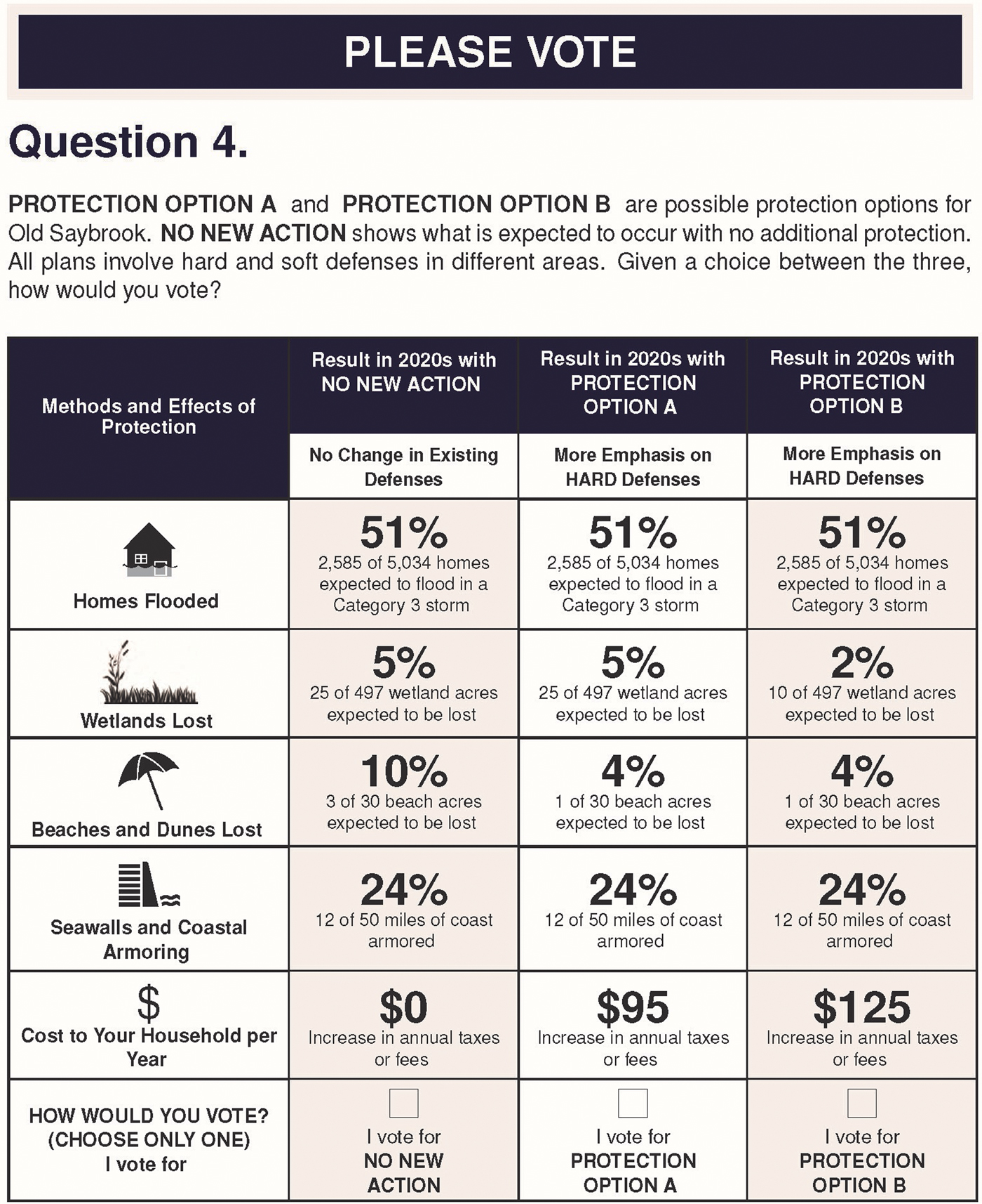
Figure 2. Sample Choice Question from Survey Version S2
Beyond the inclusion of OU, the model is specified as a traditional random utility model in which household h chooses among three options (k = A,B,N), including two multi-attribute adaptation options (A,B) and a status quo (N), with no adaptation action and zero household cost. Each option is characterized by a vector of variables, X = [X 1A, X 1B…X J] representing coastal adaptation outcomes. Variables X 1A, X 1B…X J−1 represent non-monetary adaptation outcomes, including the number of homes expected to flood in storms of different intensity, and X J represents unavoidable household cost. The vector P x1 represents a set of probabilities associated with home flooding attributes X 1Ak and X 1Bk. We represent the utility of household h from option k as
 $$\; U_{hk}\lpar X_{1Ak}\comma \; X_{1Bk} \ldots X_{Jk}\comma \; P_{x1}\rpar = u_{hk}\lpar X_{1Ak}\comma \; X_{1Bk} \ldots X_{Jk}\comma \; P_{x1}\rpar + \; \varepsilon _{hk},$$
where U hk is the utility derived by household h from option k; U hk (.) is a function representing the empirically measurable component of utility, and εhk is the unobservable component of utility and modeled as econometric error.Footnote 10
If one assumes that outcomes are certain or that respondents maximize linear expected utility (e.g., are risk neutral), equation 1 may be specified using an additively separable, linear functional form. The resulting model may be estimated using maximum likelihood models for discrete outcomes (e.g., conditional, mixed, or generalized mixed logit), with likelihood functions determined by assumptions regarding such factors as the unobservable component of utility, scale heterogeneity, and preference heterogeneity (Hensher and Greene Reference Hensher and Greene2003, Train and Weeks Reference Torres, Faccioli and Font2005, Train Reference Train2009, Fiebig et al. Reference Fiebig, Keane, Louviere and Wasi2010).
Models such as (1) may also be estimated using non-linear (in the parameters) functional forms that allow for behavior beyond risk neutral expected utility maximization (Glenk and Colombo Reference Glenk and Colombo2013). Here, such models cannot be estimated because (as noted above), the probabilities of Category 2 and 3 storms are exogenous and fixed within our data, such that P L and P H are scalars (respondents were provided information on actual storm probability, which does not vary across the case study area). Hence, we proceed with estimation using a linear expected utility framework, while noting that models allowing for non-linear risk preferences may be more appropriate when probabilities vary across respondents or scenarios.
Given the structure of storm probabilities and home flooding specified above, a linear expected utility model for version S1 reduces to the general form
 $$U_{hk} = {\rm \alpha} _{1Ah}\lpar P_L + P_H\rpar X_{1Ak} + {\rm \alpha} _{1Bh}P_HX_{1Bk} + \mathop \sum \limits_{\,j = 2}^J {\rm \alpha} _{\,jh}X_{\,jk} + \; {\rm \varepsilon} _{hk}\comma \; $$
because homes of type X 1A are expected to flood in either a Category 2 or 3 storm, whereas homes of type X 1B are only expected to flood in a Category 3 storm. However, given that P L and P H are fixed, equation 2 may be further simplified to
 $$U_{hk} = {\rm \beta} _{1Ah}X_{1Ak} + {\rm \beta} _{1Bh}X_{1Bk} + \mathop \sum \limits_{\,j = 2}^J {\rm \beta} _{\,jh}X_{\,jk} + \; {\rm \varepsilon} _{hk}\comma \; $$
where β1Ah = α1Ah(P L + P H), β1Bh = α1BhP H, and αjh = βjh. Equations 2 and 3 are structurally and statistically equivalent when P L and P H are constant; the only difference is the interpretation of parameter estimates.
Grounded in utility of the form shown in (3), our primary hypotheses relate to whether or not and how a more continuous treatment of OU in DCEs influences results. The model leads to three primary hypotheses. First, if estimated marginal utilities (and associated implicit prices) are robust to OU reframing (assuming representative samples from the same population and that utility may be modeled using a linear approximation), then the marginal utility for X 1B in S1 should be equal to that for X 1 in S2; both reflect WTP to protect a marginal home that would otherwise be flooded in a Category 3 storm. This is the first hypothesis to be considered. That is, do the different treatments of OU lead to different inferences regarding marginal WTP for home protection? One may also consider similar comparisons for other model attributes, including whether variations in OU treatment influence other, non-risky attributes within the DCE.
If marginal utilities for X 1A and X 1B differ significantly within version S1, it would further suggest that there are potentially policy-relevant welfare differences that are obscured by the version that aggregates these two types of homes into a single category. This is the second hypothesis to be tested. That is, does the marginal WTP to prevent home flooding depend on the relative degree of flood risk facing those homes? Note that there are intuitive reasons for the implicit prices for X 1A and X 1B to differ. For example, in addition to the greater probability of a Category 2 storm relative to a Category 3 storm (which influences utility as shown in [2] and [3] above), respondents might have fundamentally different preferences for protecting higher- versus lower-risk homes.
Note that these and other hypothesis tests involve implicit prices defined as ex ante compensating surplus measures; they reflect WTP before uncertainty regarding future storm events is resolved (Just, Hueth, and Schmitz Reference Just, Hueth and Schmitz2005). For example, an implicit price for X 1 would represent ex ante WTP for a policy that would protect a marginal home from flooding if a Category 3 storm occurs, where a Category 3 storm has a given probability of occurrence. Here, this is implied by the structure of (3), in which β1Ah = α1Ah(P L + P H) and β1Bh = α1BhP H, such that β1Ah and β1Bh embed the fixed probability of storm occurrence. These welfare measures are not equal to ex post measures of compensating surplus, which would reflect WTP for a guarantee that the same homes will be prevented from flooding with 100 percent certainty. Results should be interpreted accordingly.
The third and final hypothesis to be tested concerns the presence of symptoms of greater complexity within version S1. Unlike the first and second hypotheses, the third hypothesis is not evaluated using a single test, but rather is evaluated using a weight of evidence that considers multiple symptoms of task complexity across the two models, such as measures of model fit, symptoms of decision heuristics, and the prevalence of related behaviors such as extreme and/or random preferences (e.g., as captured by variations in scale). These are discussed as part of the description of the empirical model below.
Note that the focus of this paper is distinct from most DCE studies that address OU: Its goal is not to estimate the effect of varying numerical and/or verbal risk information on choices; this issue has been addressed by numerous papers in the literature (e.g., Roberts, Boyer, and Lusk Reference Roberts, Boyer and Lusk2008, Rolfe and Windle Reference Rolfe and Windle2009, Reference Rolfe and Windle2015, Shaw and Baker Reference Shaw and Baker2010, Phillips Reference Phillips2011, Glenk and Colombo Reference Glenk and Colombo2013). Here, the same underlying probabilities (i.e., the actual probabilities of Category 2 and 3 storms) are relevant to utility change under any adaptation option, and these probabilities cannot vary across choice scenarios. For this reason, the DCE holds probabilities (i.e., the probabilities of different intensity storms) constant across all surveys and scenarios and describes these probabilities explicitly on a separate page prior to choice questions.Footnote 11 This format is fundamental to the objective of the analysis. Studies that allow for only two possible outcomes of the OU-related attribute while embedding exogenously varying probabilities in valuation scenarios cannot easily isolate the effect of OU reframing from the effect of varying numerical risk information. The risk communication format adopted in this study is designed to isolate the effect of OU reframing, independent of whether and how probabilities vary across scenarios.Footnote 12
Empirical Application
We implement the model using a DCE, addressing preferences for coastal flood adaptation, including the protection of homes and natural systems such as beaches and salt marshes. The DCE was developed over two years in a process involving economists and natural scientists; meetings and interviews with town planners and community officials, engineers and stakeholder groups; and 13 focus groups with residents. Issues considered during focus groups included but were not limited to: (a) respondents’ understanding of the coastal adaptation policy context, (b) adaptation outcomes most relevant to respondents, (c) the interpretation of valuation scenarios, including any symptoms of scenario adjustment (Cameron, DeShazo, and Johnson Reference Cameron, DeShazo and Johnson2011), (d) respondents’ understanding of information presented by the questionnaire, including risk information, and (e) cognitive processes used to answer DCE questions. The first version of the survey instrument was developed after input from four initial focus groups that helped define attributes and scenarios to be considered. Later focus groups led to extensive questionnaire improvements, including updates to information provision, DCE attribute definitions, the set of attributes included, and the communication of OU.Footnote 13 Additional details of pretesting conducted in focus groups are described below. Particular attention was given to the provision and understanding of information on storm probability and associated flooding.
Prior to administration of choice questions, both survey versions provided identical text describing the historical frequency of Category 2 and 3 storms in Old Saybrook and the numerical probability that a storm of each intensity would occur at least once by the mid-2020s (based on historical frequencies). These probabilities were calculated from historical patterns of Category 2 and 3 storms over the previous 75 years, leading to an approximate 20 percent probability that at least one Category 3 storm would occur in the region by 2025, and a parallel 55 percent probability of at least one Category 2 storm. To ensure that respondents understood relationships between storms of different intensities and home flooding, questionnaire version S1 (with two risk-related attributes X 1A and X 1B) included Figure 3, a simple graphic illustrating the risk-related differences between these two groups of homes. This figure also clarified the definition of these two groups of homes, for example highlighting that they are independent and non-overlapping groups. Respondents’ understanding of this information was tested in focus groups.

Figure 3. Illustrates the Difference between the Two Home Groups in Survey Version S1
Both survey versions also provided identical information describing tradeoffs associated with alternative approaches to coastal adaptation, along with projected inundation scenarios in the mid-2020s and baseline (status quo) effects with no new adaptation actions. The data used to inform choice scenarios and inundation models (i.e., future storm and inundation scenarios) were provided by the Center for Climate Systems Research at Columbia University, NASA's Goddard Institute for Space Studies, the National Oceanic and Atmospheric Administration (NOAA) Services Center and The Nature Conservancy (TNC), as reflected in coastal flooding scenarios for TNC's Coastal Resilience platform (http://www.coastalresilience.org) (Beck et al. Reference Beck, Gilmer, Ferdaña, Raber, Shepard, Meliane, Stone, Whelchel, Hoover, Renaud, Sudmeier-Rieux and Estrella2013).
This and other information was conveyed via a combination of text, custom-designed graphics, geographic information system (GIS) maps, and photographs. Detailed instructions were also provided, including reminders to consider budget constraints and statements highlighting consequentiality (Carson and Groves Reference Carson and Groves2007). Survey language and graphics were subject to extensive pretesting in focus groups and cognitive interviews (Johnston et al. Reference Johnston, Weaver, Smith and Swallow1995, Kaplowitz, Lupi, and Hoehn Reference Kaplowitz, Lupi, Hoehn, Presser, Rothget, Cooper, Lesser, Martin, Martin and Singer2004), including the use of verbal protocols to gain insight into respondents’ comprehension and decision processes (Schkade and Payne Reference Schkade and Payne1994). This helped ensure that language, graphics and format were understood, that respondents and researchers shared interpretations of terminology and scenarios, and that scenarios captured outcomes viewed as relevant and accurate.
In questionnaire version S1, choice options are characterized by seven attributes: the percentage and number of homes expected to flood only in a Category 3 storm, the percentage and number of homes expected to flood in a Category 2 storm, wetland acreage expected to be lost, beach and dune acreage to be lost, the length of coastline to be hard-armored, whether or not the overall plan emphasizes hardened coastal defenses, and unavoidable household cost (Table 2). All outcomes are forecast as of the mid-2020s. Questionnaire version S2 is identical except that it only included one attribute characterizing the percentage and number of homes expected to flood in a Category 3 storm. That is, version S1 allows for different degrees of home flooding conditional on storms of different intensity, with each storm intensity level associated with a given probability. In contrast, version S2 mirrors standard treatments by communicating homes flooded under a single binary event (storm/no storm), with one associated probability.
Table 2. Choice Experiment Attributes and Descriptive Statistics14

14 Means and standard deviations include status quo option of no adaptation action.
Following the general approach of Johnston et al. (Reference Johnston, Segerson, Schultz, Besedin and Ramachandran2011, Reference Johnston, Schultz, Segerson, Besedin and Ramachandran2012), attributes represent each adaptation method and effect in relative (percentage) terms with regard to upper and lower reference conditions (i.e., best and worst possible in Old Saybrook) as defined in survey informational materials. Scenarios also present the cardinal basis for relative levels where applicable. With the exception of hard armoring levels and household cost, relative attribute levels represent losses or flooding approaching the upper reference condition (100 percent loss or flooding), starting from the lower reference condition (0 percent loss or flooding). For example, the attribute representing the number of homes expected to flood in a Category 2 storm (homes2) is presented both as a cardinal number of homes and as a percentage relative to the total number of homes in Old Saybrook. To ensure comparability, all home flooding attributes (homes, homes2 and homes3) are denominated as a percentage of all homes in Old Saybrook, where 1 percent = 50.34 homes.
Grounded in these attribute levels, a fractional factorial experimental design was generated using a D-efficiency criterion (Sándor and Wedel Reference Sandor and Wedel2001, Reference Sándor and Wedel2002, Ferrini and Scarpa Reference Ferrini and Scarpa2007, Rose and Bliemer Reference Rose and Bliemer2009) for main effects and selected two-way interactions, yielding 72 profiles blocked in 24 booklets. Other measures of efficiency were also reviewed for each candidate design, e.g., S-efficiency, to evaluate potential sample sizes required to estimate preference parameters, for assumed utility specifications (Scarpa and Rose Reference Scarpa and Rose2008, Bliemer, Rose, and Hensher Reference Bliemer, Rose and Hensher2009, Rose and Bliemer Reference Rose and Bliemer2009). Design efficiency was also reevaluated using alternative assumptions for preference parameters and utility structure.Footnote 15 Each respondent was provided with three choice questions and instructed to consider each as independent and non-additive. Table 2 provides attribute summary statistics and definitions. Table 3 illustrates attribute levels. Sample choice questions from Surveys S1 and S2 are shown in Figures 1 and 2, respectively.
Table 3. Attribute Levels in Choice Experiment Designs (Identical for S1 and S2 Surveys)

Surveys were sent to 1,152 randomly selected Old Saybrook households via U.S. postal mail during May through July 2014, with repeated mailings following Dillman et al. (Reference Dillman, Phelps, Tortora, Swift, Kohrell, Berck and Messer2009) to increase response rates. The analysis is based on 167 returns from 493 deliverable S1 surveys, for a 33.87 percent response rate, and 163 returns from the 488 deliverable S2 surveys, for a 33.40 percent response rate.Footnote 16
Model Estimation
The models are estimated using generalized multinomial logit (GMNL; Fiebig et al. Reference Fiebig, Keane, Louviere and Wasi2010) in WTP-space (cf. Cameron and James Reference Cameron and James1987, Scarpa, Thiene, and Train Reference Scarpa, Thiene and Train2008, Thiene and Scarpa Reference Thiene and Scarpa2009, Hensher and Greene Reference Hensher and Greene2011). WTP-space estimation circumvents challenges associated with ambiguously defined welfare estimates from certain types of preference-space mixed logit specifications. These are caused by the presence of a randomly specified cost coefficient in the denominator of the WTP expression, leading to behaviorally and statistically implausible WTP values, e.g., due to infinite WTP moments (Hensher and Greene Reference Hensher and Greene2003, Train and Weeks Reference Torres, Faccioli and Font2005, Scarpa, Thiene and Train Reference Scarpa, Thiene and Train2008, Thiene and Scarpa Reference Thiene and Scarpa2009, Daly, Hess, and Train Reference Daly, Hess and Train2012). Cost coefficient distributions that lead to finite WTP moments can lead to additional challenges, such as unrealistic welfare estimates associated with the tails of the lognormal distribution (Hensher and Greene Reference Hensher and Greene2003).
The model is specified following Hensher and Greene (Reference Hensher and Greene2011), based on the WTP-space model of Scarpa, Thiene, and Train (Reference Scarpa and Rose2008) and Thiene and Scarpa (Reference Thiene and Scarpa2009). Grounded in (3), for household h facing choice alternatives k = A, B, N and t = 1…T choice sets, the model in preference space may be restated in streamlined form as
 $$U_{hkt} = {\bi B}{\bi ^{\prime}}_{\bi h}{\bi X}_{hkt} + {\rm \varepsilon} _{hkt}\comma \; $$
where Bh is a vector of random parameters underlying marginal utilities of attributes Xhkt and εhkt is a traditional i.i.d. type-one extreme-value error with constant variance. Within a random parameter preference-space model, Bh may be specified as
 $${\bi B}_{\bi h} = {\bi B} + {\bf \Gamma} {\bf \nu} _{\bi h}\comma \; $$
where Γ is a lower triangular matrix that provides the standard deviations and covariances of Bh and νh is a vector of random variables that provide the stochastic element of preference weights.
Fiebig et al. (Reference Fiebig, Keane, Louviere and Wasi2010) extend this model to distinguish the possibility that preference heterogeneity is either independent of, or proportional to, scale heterogeneity by specifying
 $${\bi B}_{\bi h} = \; {\rm \sigma} _h{\bi B} + \; {\rm \sigma} _h\lsqb {\rm \gamma} + \; \lpar 1 - \; {\rm \gamma} \rpar \rsqb {\bf \Gamma} {\bf \nu} _{\bi h}$$
 $${\rm \sigma} _h = \; {\rm exp}( - {\rm \tau} ^2/2 + \; {\rm \tau} w_h).$$
In this model, Γ and νh are as defined as above, σh is the logit scale parameter, τ is the primary parameter that determines scale heterogeneity (with w h ~ N (0,1)), and γ is a weighting parameter that lies between zero and one, governing how the variance of residual preference heterogeneity varies with scale (Hensher and Greene Reference Hensher and Greene2011). The traditional random parameters model in (4) is a special case of the GMNL model with γ = 0 and τ = 0 (the multinomial logit model arises when γ = 0, Γ = 0, and τ = 0 so that σ h = σ = 1).Footnote 17
To derive the GMNL in WTP-space, we assume that utility is separable in price, p hkt,Footnote 18 and other attributes, xhkt, and rewrite equation 4 as
 $$U_{hkt} = \lambda _hp_{hkt} + {\bf \delta} {\rm ^{\prime}}_{\bi h}{\bi x}_{{\bi hkt}} + {\rm \varepsilon} _{hkt}$$
where λh = c h/σh is the preference-space coefficient on program cost, c h is the marginal utility of income, and  ${\bf \delta} {\rm ^{\prime}}_{\bi h} = \lpar {\bf \beta} _{\bi h}/{\rm \sigma} _h\rpar {\bi ^{\prime}}$ is a conforming vector of coefficients on non-price attributes xhkt. From (8), WTP may be calculated as the ratio of the coefficient on any non-price attribute and the coefficient on cost, ωh = (δh/λh) = (βh/c h). Given this, we can rewrite (8) to derive the parallel WTP-space specification (Train and Weeks Reference Torres, Faccioli and Font2005),
 $$\eqalign{U_{hkt} &= \,{\rm \lambda} _h\lsqb p_{hkt} + \lpar 1/{\rm \lambda} _h\rpar {\bf \delta} {\rm ^{\prime}}_{\bi h}{\bi x}_{{\bi hkt}}\rsqb + {\rm \varepsilon} _{hkt}\comma \; \cr &= \, {\rm \lambda} _h\lsqb p_{hkt} + {\bf \omega} {\rm ^{\prime}}_{\bi h}{\bi x}_{{\bi hkt}}\rsqb + {\rm \varepsilon} _{ihk}\comma \; } $$
where (9) is behaviorally equivalent to (8), its preference-space analog. By setting γ = 0, the elements of the resulting vector  ${\bf \omega} {\rm ^{\prime}}_{\bi h}$ are random coefficients representing direct estimates of WTP, assumed to be normally distributed. The parameter λh becomes the normalizing constant (Hensher and Greene Reference Hensher and Greene2011), and the WTP-space model thus circumvents the need to estimate the ratio of two parameters via a direct estimate of the ratio. This specification enables the analyst to specify the assumed distribution of WTP directly (Train and Weeks Reference Torres, Faccioli and Font2005, Scarpa, Thiene, and Train Reference Scarpa and Rose2008). To ensure the positive marginal utility of income, we specify ${\rm \lambda} _h = - e^{\varphi_h} $, where ϕh = (−τ2/2 + τw h) is the latent normal factor defining the lognormally distributed cost coefficient (Hensher and Greene Reference Hensher and Greene2011).
From equation 9, additional multiplicative interactions are included between a set of socioeconomic variables and neither, the alternative specific constant for the status quo (Morrison et al. Reference Morrison, Bennett, Blamey and Louviere2002, Columbo, Calatrava-Requena, and Hanley Reference Columbo, Calatrava-Requena and Hanley2007, Johnston and Duke Reference Johnston and Duke2010). These variables included the respondent's age in years (age), and dummy variables identifying households earning more than $60,000 per year (hi_income) and respondents with at least a 4-year college degree (college). An identical specification was applied to each model, with parameters on neither and homes expected to flood (homes2 and homes3 in S1 and homes in S2) specified random, assuming normal and independent distributions. Other parameters are specified as non-random.Footnote 19 The sign of the cost variable was reversed prior to estimation. Models were estimated with different starting values and numbers of Halton draws to evaluate robustness and local versus global convergence. Parallel preference-space models were estimated to further evaluate the robustness of results; these lead to similar conclusions as models reported in the main text below (see appendix). The final model is estimated using 500 Halton draws.
Results
Results are reported in Table 4. Two models are illustrated, corresponding to versions S1 and S2. Estimated WTP coefficients from versions S1 and S2 are jointly significant at p ≤ 0.0001 (χ2 = 163.52, df = 16 and χ2 = 186.94, df = 14). Signs of estimated coefficients are identical in both versions, with the exception of coefficient estimates on seawalls (length of coastline to be hard-armored by the mid-2020s). The sign of all coefficient estimates match prior expectations, where prior expectations exist.Footnote 20 All main effect coefficient estimates are statistically significant in version S2. In version S1, all are significant except for the coefficients on neither and hard. In version S1, coefficient estimates on all socioeconomic interaction terms with the ASC are statistically significant, except for that on ne × hi_income. In version S2, only the coefficient estimate on ne × college is statistically significant.
Table 4. Results of WTP-Space Generalized Multinomial Logit Models

a Results show the means and standard deviations of the simulated empirical distributions of implicit price differences. For homes2 and homes3, WTP(S1)–WTP(S2) tests WTPhomes2 − WTPhomes and WTPhomes3 − WTPhomes.
***, **, * imply significance at 1 percent, 5 percent and 10 percent level.
For continuous attributes (homes, homes2, homes3, beaches, wetlands, seawalls), coefficients reflect mean implicit prices (marginal WTP) per percentage point increase, along with the standard deviations of these implicit prices (for random parameters). For example, within version S1, annual per-household WTP per percentage point increase in homes2 is −$6.75, implying that the average household is willing to pay $6.75 to avoid a one-percentage-point increase in homes expected to flood in a Category 2 storm. Similarly, in version S2, the average household is willing to pay $7.36 to avoid an identical magnitude increase in homes expected to flood in a Category 3 storm.Footnote 21 The coefficient estimate on binary attributes such as hard and the ASC neither reflect the mean implicit price for the presence of these attributes relative to their absence. In version S2, for example, the coefficient estimate of −76.56 on hard suggests that the average household is willing to pay $76.56 annually to avoid adaptation action that emphasizes hard, engineered defenses.
Model results also provide insight into preference heterogeneity. For example, results for versions S1 and S2 suggest statistically significant WTP heterogeneity for neither, along with systematic variation in WTP associated with sociodemographic variables. Version S1 finds WTP homogeneity for homes2 and homes3, whereas version S2 finds significant WTP heterogeneity for homes. Additional discussion of parallels and differences between the two models is provided below.
Overall, the two versions lead to similar general conclusions regarding WTP for adaptation outcomes. These conclusions are consistent with both intuition and results from focus groups. Further, viewed in isolation, both survey versions generate seemingly reasonable WTP estimates (with the exception of results for the ASC in version S1, discussed below). However, despite these general similarities, differences between the two models suggest that the treatment of OU can have non-trivial implications for welfare estimation and choice complexity. The remainder of this paper focuses on these differences, oriented around the three hypotheses described above.
Effects of OU Treatments
Differences between coefficient estimates from versions S1 and S2 are tested using a parametric, empirical convolution of estimate distributions, with significance levels determined through percentiles on the resulting distributions (Poe, Giraud, and Loomis Reference Poe, Giraud and Loomis2005). Implicit price differences are reported as the mean of the resulting simulated distributions (of differences); these hence differ slightly from point estimate differences in WTP means. For the home flooding attributes (where attributes differ across S1 and S2), we test whether implicit prices for either homes2 or homes3 in S1 (WTPhomes2, WTPhomes3) are equal to the implicit price for homes in S2 (WTPhomes). Other than the expected relationship between WTP for X 1B in S1 and X 1 in S2 (discussed above), theory provides ambiguous guidance regarding the expected relationship among these three measures of WTP. Nonetheless, these findings are relevant to whether or not and how OU treatments influence welfare estimates.
Results are shown in the last column of Table 4. Tests for the first hypothesis lead us to reject convergent validity for roughly half of coefficient estimates: ne × age, ne × college, hard, seawalls, and homes3 (in version S1) and homes (in version S2) are statistically different between versions S1 and S2. For example, we find relatively large and statistically significant implicit price differences for the binary variable hard ($55.50; p < 0.10) and the multiplicative interaction terms ne × age and ne × college (−$6.24 and −$288.37, respectively). That is, when compared across models, alternative treatments of OU for home flooding appear to have an effect on mean implicit prices for multiple adaptation outcomes, including those for the home flooding attributes (homes, homes2 and homes3).
Versions S1 and S2 also lead to different conclusions regarding implicit price standard deviations associated with home flooding. We find statistically insignificant standard deviation estimates for homes2 and homes3 in S1. In contrast, the standard deviation estimate on homes in S2 is statistically significant. These differences in estimated standard deviations across models are statistically significant at p < 0.01 (i.e., between the standard deviations of homes2 and homes, and between homes3 and homes). Simply put, when home flooding OU is discretized using a single variable (homes), we estimate an implicit price with heterogeneity around the mean; this apparent heterogeneity disappears when OU is discretized using two variables (homes2, homes3).Footnote 22
Considering the second hypothesis, we also reject the null hypothesis that WTPhomes2 = WTPhomes3 in version S1 (Wald χ2 = 3.41; p ≤ 0.0648). As discussed above, there are multiple reasons to expect that these implicit prices might differ,Footnote 23 although theory provides ambiguous guidance regarding the sign and magnitude of differences. Regardless, the finding that these implicit prices are not identical suggests that version S1 (the more accurate representation of OU) reveals information about respondents’ risk preferences that is not provided by version S2. Results suggest that residents are willing to pay $4.84 more per percentage point reduction in the number of homes expected to flood only in a Category 3 storm than they are for the same reduction in homes expected to flood in Category 2 storm.
This result is particularly interesting because the ex post number of homes prevented from flooding is expected to be greater from a one percentage point change in homes2 than for homes3 (once the uncertainty is resolved). Despite this, we find that |WTPhomes2| < |WTPhomes3|. This result is consistent with focus group results suggesting that Old Saybrook residents view the protection of homes at very high flood risk (e.g., homes2) to be the primary responsibility of the homeowners who purchase this high-risk property. In contrast, residents feel more of an altruistic motive to protect homes in lower-risk locations (homes3).Footnote 24 Hence, the value per certain home protected is expected to be less for homes2 than homes3, leading to the implicit price patterns of Table 4.Footnote 25
These findings suggest that the more accurate discretization of OU underlying version S1 may generate additional insights—and different information—than the simpler two-outcome discretization underlying version S2. Results also demonstrate that variations in OU framing for a single attribute (here, home flooding) can lead to non-trivial differences in welfare estimates associated with other model variables, even when other aspects of DCE scenarios are held constant.
The third hypothesis concerns whether or not there are symptoms of additional choice complexity in responses to version S1. Here, there is some evidence that version S1 presented a more complex choice task, leading to greater application of choice heuristics. For example, the very large estimated standard deviation for neither in version S1 suggests the potential presence of serial choice behavior (or serial participation / non-participation), in which a subset of respondents universally accepts or rejects most or all status quo options, regardless of other attributes (Kriström Reference Kriström1997, von Haefen, Massey, and Adamowicz Reference Von Haefen, Massey and Adamowicz2005). Behavior such as this is often interpreted as a sign of task complexity, in which “the complexity of a decision may preclude the use of all available information” (Mazzotta and Opaluch Reference Mazzotta and Opaluch1995, p. 500).
The combined magnitudes of the implicit prices associated with neither, ne × age, ne × hi_income and ne × college provides an additional sign of complexity associated with version S1. For example, given a mean age of 58 among version S1 respondents, the mean combined point estimate of WTP associated with the status quo option (neither = 1 versus 0) for college-educated respondents is −$983.70, holding all else constant. This improbably large magnitude also suggests that choices may have been influenced by decision heuristics inconsistent with fully compensatory decision-making (e.g., serial anti-status-quo choices).
In contrast, the statistical significance of τ in equation 7 does not suggest additional complexity of version S1. This parameter may be interpreted as the degree to which scale varies across the sample (Fiebig et al. Reference Fiebig, Keane, Louviere and Wasi2010), or the degree of respondent-specific variation in choice randomness or inconsistency within the sample.Footnote 26 Although the point estimate of τ is 45 percent greater in version S1 than S2 (−2.35 versus −1.62), the difference between these estimates is not statistically significant. This result suggests that scale variation across respondents is statistically indistinguishable between the two versions.Footnote 27
Similar findings emerge from multiple alternative WTP- and preference-space model specifications. For illustration, the appendix reports the results of parallel specifications estimated using a mixed logit preference-space model that holds scale constant. Results are generally consistent with those reported above, with variations in marginal utility estimates and statistical significance that are similar to those found in the WTP-space GMNL models (Table 4).Footnote 28 Welfare estimates from these models also show similar patterns.
These results highlight potential challenges facing stated preference valuation of outcomes subject to non-trivial OU. Results show that standard two-outcome treatments may suppress some policy-relevant aspects of preferences that are revealed when OU is presented with greater accuracy. That is, the methods used to discretize OU are not welfare-neutral. However, our results also suggest that this additional welfare information may come at a cost of higher task complexity and prevalence of choice heuristics, with symptoms including large implicit prices and implicit price standard deviations associated with the status quo ASC. At the same time, roughly half of implicit price estimates were invariant to the alternative OU treatments. This is an encouraging outcome, suggesting that some welfare inferences from DCEs are robust, notwithstanding other potential tradeoffs associated with alternative approaches to OU framing.
Conclusions
Results of the models shown above suggest the need for additional research on the effect of alternative approaches to OU discretization within DCEs. This is an area that has been subject to relatively little research in the literature, despite the relative frequency with which DCEs address outcomes subject to OU. We also, however, emphasize that the results presented here are specific to our case study of coastal hazard adaptation, and that similar findings may or may not apply to other contexts. For example, case studies addressing very familiar topics and risks might enable respondents to more easily process additional OU resolution. In addition, results might vary in cases where outcome probabilities change across scenarios, as opposed to the present application in which probabilities are purposefully fixed. These and other caveats aside, the present results suggest that increases in the resolution and accuracy of OU framing within DCEs may require the development of novel methods that enable respondents to understand more accurate probability distributions without concomitant increases in scenario complexity. Pending the development of such methods, researchers may wish to consider the possibility that DCE results may be conditional on the number of intervals used to present OU.
Appendix
Table A1 reports a preference-space, mixed logit counterpart of the WTP-space GMNL models reported in Table 4, estimated to evaluate the robustness of results reported in the main text. Identical specifications were again applied to both DCE versions: parameters on cost, neither, homes2 and homes3 (in S1), and homes (in S2) were specified random and normally distributed, with cost sign-reversed prior to estimation. Estimated coefficients in versions S1 and S2 are again jointly significant at p ≤ 0.0001 (χ2 = 153.86; df = 15 and χ2 = 115.78; df = 13) with pseudo-R2 values of 0.21 and 0.15, respectively. Here, main effect coefficient estimates are interpreted as relative marginal utilities.
Table A1. Results of Preference-Space Mixed Logit Models

Across both models, the signs and statistical significance of coefficient estimates are again identical. The only exception is the significance associated with the main effect coefficient estimates on wetlands, which is borderline insignificant in version S1 (Table A1). Most findings of the preference-space models are consistent with results in the main text. There are a few differences in the statistical significance of coefficient estimates between these results and those reported in the main text; these are not surprising given the high level of scale heterogeneity present in both survey versions (preference-space mixed logit models do not account for such variation). Results of these preference-space specifications yield the same general conclusions regarding the effect of OU discretization, with (a) many resulting welfare estimates different across versions S1 and S2, and (b) additional evidence of complexity in version S1.


 Open access