Introduction
The Baltic Air-Sea-Ice Study (BASIS) is a sub-project of the Baltic Sea program BALTEX of the World Climate Research Programme/Global Energy and Water Cycle Experiment (WCRP/GEWEX). It is carried out by Finnish, Swedish and German institutes. Observations for validation and optimization of the thermodynamic ice model were performed during the BASIS field campaign in the northern Baltic Sea in 1998. The goals of the project include an investigation into air-ice-ocean coupling and its modelling (Reference LauniainenLauniainen, 1999).
A one-dimensional, multi-layer sea-ice model was created in the Finnish Institute of Marine Research (FIMR) to study ice thermodynamics and air-ice-sea coupling (Reference Cheng and LauniainenCheng and Launiainen, 1998; Reference Launiainen and ChengLauniainen and Cheng, 1998). Overall, the model is similar to those of Reference GabisonGabison (1987) and Reference Ebert and CurryEbert and Curry (1993). The main physical processes expressed in the model involve the air-ice coupling, heat fluxes and heat balance at the surface and the ice bottom, heat conduction in the multi-layer snow and ice, and mass balances at the surface and the bottom. The model is shown schematically in Figure 1. Model solutions are obtained using the following procedures:
-
(1) The turbulent air-ice fluxes of momentum, sensible and latent heat are calculated on the basis of Monin-Obukhov similarity theory. Integration of the non-dimensional universal profile gradients of wind speed (V), temperature (T) and moisture (q) yield the vertical profiles of V(za), T(za) and g(za) in the surface boundary layer (SBL).
-
(2) Various heat fluxes, i.e. the net downward shortwave radiation (1 - α)Qs, the shortwave absorption in snow and ice (I), the downward (Qd) and upward (Qb) longwave radiation, the sensible heat (Qh), the latent heat (Qie) and the surface conductive heat flux (Fc), are used to construct a heat- and mass-balance equation for the surface layer of ice or snow. This balance serves as the upper boundary condition needed to describe heat conduction in the ice. The surface temperature (Tsfc) is the critical quantity to be iterated in the solution of the surface heat balance. Surface melting (Ah,) is a response to the surface heat balance when the surface temperature tends to increase above the freezing point.
-
(3) The temperature profile in the ice Ti(z, t) is numerically solved from the heat-conduction equation. The upper boundary condition is the surface temperature, and the lower boundary condition is the freezing temperature (Tf) at the ice bottom. Absorption of shortwave radiation I(z) in the snow and ice is an additional source term in the heat-conduction equation. The volumetric heat capacity (pc)si and the heat conductivity of sea ice (ksi) are functions of ice salinity (si) and temperature. In the case of a thin snow cover, 0 < hs < 0.01 m, a single snow layer (Qsi, hs) is coupled with ice. For snow thickness of > 0.01m, the heat-conduction equation is also applied to calculate temperatures (Tsnow) at various depths in the snow. The snow/ice interface temperature (Tin) is calculated according to the flux continuation assumption (Fc = Qsi).
-
(4) The difference between the heat flux from the ocean mixed layer (Fw) and conduction upwards from the ice bottom (Qc) determines the ice growth or melt (±Δhi) at the ice bottom.
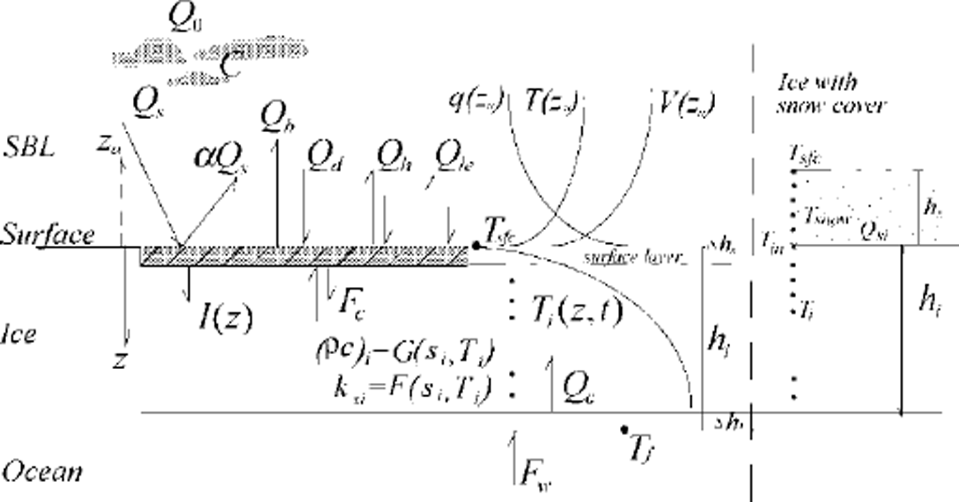
Fig. 1. Structure of the FIMR one-dimensional thermodynamic sea-ice model. For symbols, see the text.
Field Data and Model Parameters
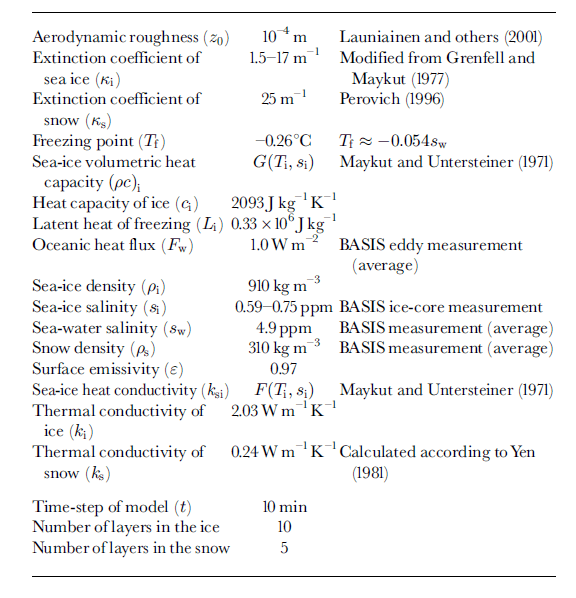
The BASIS field experiment was carried out from 16 February to 7 March 1998 in the Baltic Sea. The central ice station was located in a coastal fast-ice zone, near the anchored Finnish vessel r/v aranda. Observations of wind speed, air temperature and relative humidity were made from a sea-ice weather mast. The 10 min averages of these quantities served as the forcing data for the ice model. The data time series are shown in Figure 2. Cloudiness (C) was observed visually every 3 hours. Downward and upward shortwave and longwave radiation were measured during BASIS, but 4.2 days of these measurements are missing due to bad weather conditions. Large variations were observed in the surface albedo; the measured shortwave radiation and albedo values were used for the model input. In the case of missing data, r/varanda’s shortwave radiation measurements and an average albedo of 0.73 were used. A thermistor string with 11 sensors was deployed vertically through the snow and ice. The temperatures of near-surface air, snow, ice and sea water near the ice bottom were measured at various levels. The installation of the thermistor string and its sensors are shown schematically in Figure 3, indicating the initial and final stages in the ice. Snow and ice thickness were measured manually once a day at 10 locations near the thermistor string. The daily means of snow thickness were interpolated linearly and used as model input. A sonic anemometer (Metek) was also deployed, and eddy fluxes of sensible heat and momentum were measured. For a short-period simulation, the model parameters were specified to correspond to the BASIS field characteristics; these are given in Table 1 (note that the salinity of the Baltic Sea ice is much less than that of the sea ice in the oceans). In this study, oceanic heat flux was specified as an input for the model. Eddy-flux measurements performed in the water near the ice bottom suggested that there was, on average, a small upward heat flux (1.0 Wm−2) during BASIS. Its small magnitude is explained by the strong water stratification below the ice in the Baltic Sea. In the simulation, we initialized the model with the weather forcing of BASIS and with the observed solar radiation until a stable vertical temperature profile in the snow and ice was achieved.
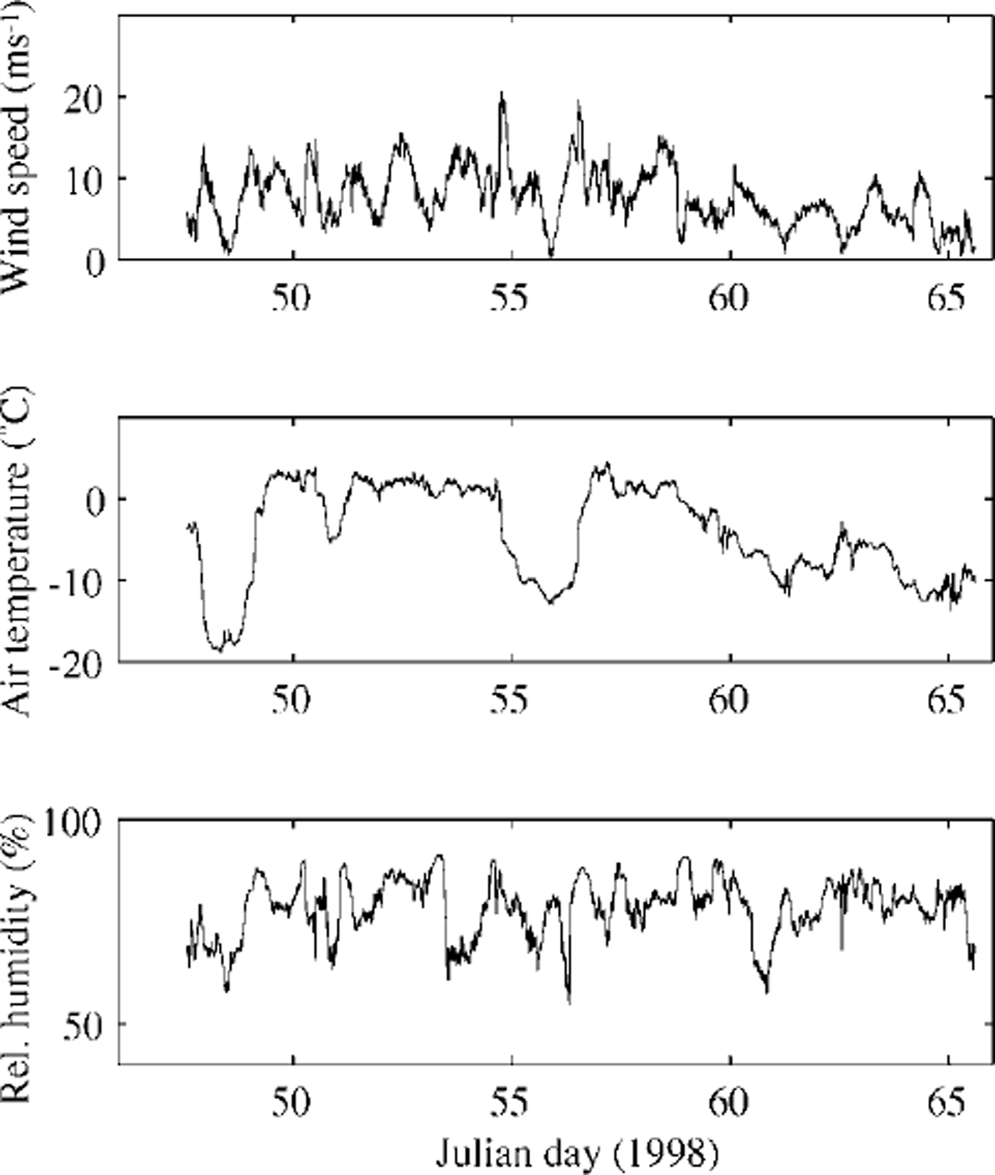
Fig. 2. Time series of wind speed (at 10 m), air temperature (10 m) and moisture (4.6m) during basis
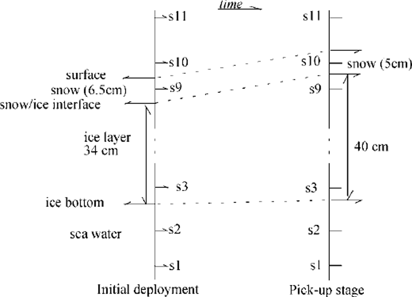
Fig. 3. Geometric location of sensors attached to an ice thermistor string in the air/snow surface, snow/ice interface and ice/water. at the beginning, sensor s10 was 1.5 cm above the surface. the snow depth was 6.5 cm (3 cm soft snow + 3.5 cm hard snow) measured from the surface of the ice. the ice thickness was 34 en. s3 was 5 cm from the ice bottom. at the end of basis, s10 was situated 3.5 cm below the snow surface. the snow/ice interface was 1.5 cm below s10, and the total ice thickness was 40 cm. a distance of 4.5 cm was measured between s3 and the ice bottom.
Table 1. Model parameters based on basis measurements and the literature
Results
The measured downward solar radiation in the midday period showed several large peaks. For comparison, it was also calculated (Fig. 4) using an empirical sinusoidal formula taking the observed cloudiness into account, i.e. qs = q0(−0.52Q, where q0 was calculated from Reference ShineShine’s (1984) formula for clear skies, and (1−0.52Q is a cloudiness factor given by Reference BennettBennett (1982). Differences may be due to multiple scattering between the snow surface and clouds. During the occurrence of the large peaks, the cloud cover was 0.5−1; large peaks were also present in r/v aranda’s shortwave radiation data. According to several authors (Reference Schneider and DicksonSchneider and Dickson, 1976; Reference ShineShine, 1984; Reference Wendler and EatonWendler and Eaton, 1990), neglect of multiple scattering may lead to errors of 30−60% in the surface shortwave radiation flux. Several parameterization of downward longwave radiation are included in the ice-model code for comparison. The parameterization of Reference PrataPrata (1996), combined with the cloudiness factor of Reference Jacobs, Barry and JacobsJacobs (1978), was selected for this study. Comparison of the observed and calculated net longwave radiation flux is shown in Figure 5. Differences were mainly related to the estimation of downward longwave radiation, especially during the period before day 55 when the air temperature was above freezing point and melting was predicted by the model. In the later part of the period, the calculations compare somewhat better with the measurements. A comparison of modelled eddy fluxes of momentum and sensible heat and those measured by the sonic anemometer is shown in Figure 6. The results indicate that the ice model simulates these fluxes quite well. The mean values of the various surface fluxes are given in Table 2. The observed and modelled in-ice temperatures are compared in Figure 7. The thermistor-string measurements indicated snow-ice formation near the surface (Fig. 3). At the beginning of the period, a large vertical gradient is seen in the experimental in-ice temperature profile (Fig. 7a), indicating rapid freezing around the thermistor string after its installation. This was not well simulated by the ice model (Fig. 7b) because the installation of the thermistor string caused water flooding near the surface, which was not taken into account in the model initialization. The modelled average in-ice conductive heat flux was 10.7 W m−2 upward, while the thermistor-string measurement indicated an average upward heat flux of 8.1 W m−2 . The difference may be due to the inaccuracy of the estimated heat conductivity and the complexities of the snow cover above ice. However, the results (Fig. 7b) still indicate an encouraging agreement with the observed thermal structure and its time development. The modelled air/snow interface temperature was compared with the radiation measurement-derived surface temperature, and with estimates derived from the flux-profile relationships (Reference Launiainen, Bin, Uotila and VihmaLaumainen and others, 2001). The results indicate that the ice model can generally reproduce the surface temperature well. However, in cases of small surface heat fluxes, the surface boundary is flux-controlled in the model, and the modelled surface temperature may be less accurate. The measured snow and ice and modelled ice-thickness variations are shown in Figure 8. The measurements of snow and ice show distinct spatial and temporal variations in the test area, due to highly variable weather during the BASIS experiment. The surface melting largely occurred when measured air temperatures were above freezing. Figure 8b shows the time series of the modelled surface melting, producing a cumulative snow-thickness change of about 12 cm. Figure 8c gives the modelled ice growth at the ice bottom, leading to a 3 cm increase in thickness. Figure 8d shows the simulated ice thickness compared with the measurements. Assuming the surface meltwater is totally refrozen, and the density ratio between the snow and sea ice is 0.35, the above modelled melting would correspond to about 5 cm of snow-ice formation. In practice, however, instead of immediately refreezing, melting water percolates into the snow/ice interface and may be mixed with snow to form a slush layer, which later will be refrozen under the right weather conditions. Such a layer of slush or snow ice will affect the heat conduction and heat flux through the whole ice layer. These uncertainties may cause discrepancies between the measurements and modelling of ice temperature and ice thickness. Further studies on this aspect are needed.
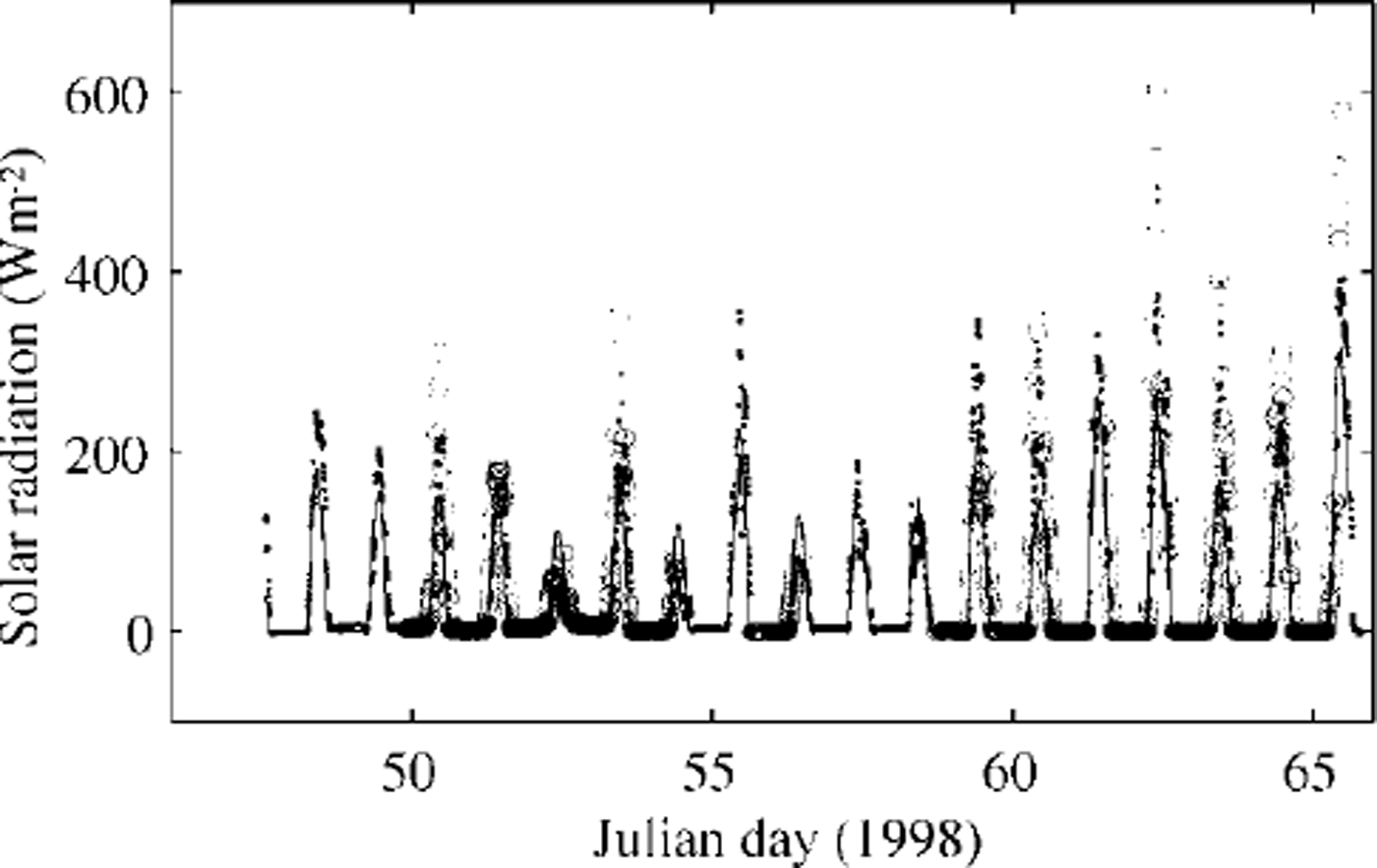
Fig. 4. Measured and estimated shortwave radiation. Circles indicate measurements by the radiometer over the sea ice, and solid dots measurements on the R/V Aranda. The solid line gives the results calculated using an empirical formula. The model calculations use the measured values.
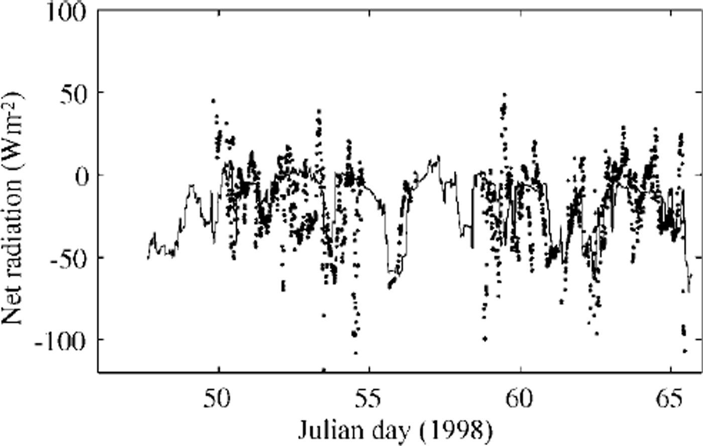
Fig. 5. Net longwave radiation flux comparison. the solid line gives the ice-model estimate, and dots are the observed values.
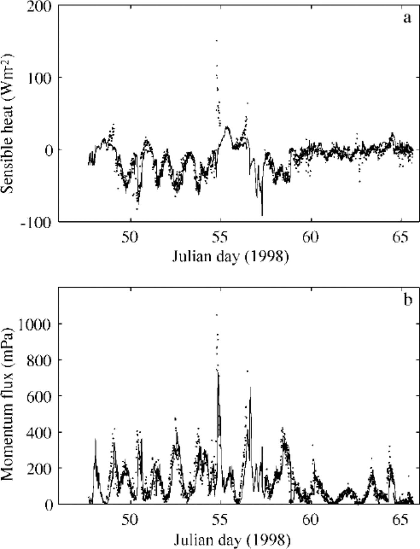
Fig. 6. Modelled (solid line) turbulent surface fluxes of sensible heat (a) and momentum (b) compared with those measured as eddy fluxes by the some anemometer (dots).

Fig. 7. Internal ice temperatures (°c) during the basis experiment, (a) observed m-ice temperatures. circles indicate the locations of sensors attached to the thermistor string, (b) in-ice temperatures calculated by the ice model. the three horizontal lines show the average observed (a) and modelled (b) evolution of the height/depth of the snow surface, the snow/ice interface and the ice bottom.
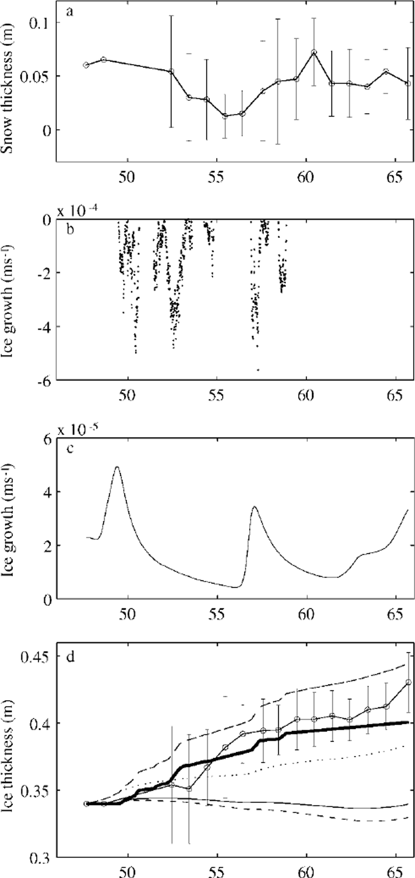
Fig. 8. (a) observed mean snow thickness (circle-connected line) with ± standard deviation (vertical bars), ( b) modelled melting rate at the surface, (c) modelled freezing at the ice bottom, ( d) observed mean ice thickness (circle-connected line) with ± standard deviation (vertical bars). the dotted line gives the modelled ice growth at the bottom, and the thick line gives the ice growth solely due to snow/ice transformation. the broken line on top is the cumulative ice growth. the lowermost two lines (solid and broken) give the ice-thickness variation calculated from the ice-bottom heat mass balance using thermistor-string temperature data with an assumed average oceanic heat flux of 1 and 2 wm−2, respectively.
Table 2. Observed and calculated mean values of various surface heat. fluxes

Some comparative estimates can be made from the measured ice-thickness and ice-temperature data (Reference Wettlaufer, Untersteiner and ColonyWettlaufer and others, 1990). At the ice bottom, a heat balance is achieved between heat conduction, latent heat of fusion and oceanic heat flux. Accordingly, the heat/mass balance reads: ρili∂hi/∂t = ki∂ti/∂z - fw. The thermistor-string measurements (Fig. 3) indicate an approximate mass equilibrium during BASIS with no effective thickness change at the ice bottom. Using the modelled thermal structure and heat conduction near the ice bottom, this equilibrium corresponds to an average oceanic heat flux of 0.63 W m−2. On the other hand, assuming a small average oceanic heat flux and calculating the heat conduction near the ice bottom from the measured temperature profile, the ice thickness controlled by the bottom heat/mass balance would be in approximate equilibrium for fw = 1W m−2 and indicates a melting of about 1 cm for fw = 2 W m−2 (Fig. 8d). The ice equilibrium for fw = 1W m−2 agrees with the ice-thickness measurements by the thermistor string and with the below-ice eddy-flux measurements.
The model input quantities for this simulation showed large temporal variations, especially in solar radiation and surface albedo. The ice model was forced by the observed shortwave radiation, and this produced better results than a control run using the parameterized values. This was concluded from comparisons of the observed and modelled surface temperature and net radiation, which were measured independently of the shortwave radiation. As for the model initialization, if we assume a constant vertical temperature profile of −0.5°C in the ice, the in-ice temperature adjustment would cause a difference in ice-growth rate in the first 2 days of simulation and eventually a 20% change in the overall ice thickness compared with the current model run. In addition, the estimation of the thermal heat conductivities of ice and snow is of primary importance for the modelling of ice thermodynamics. In this study we used a simple parameterization. Potential errors due to this inaccuracy may remain in the model results with respect to the in-ice conductive heat flux. Further data on the heat conductivity are needed.
Conclusion
An 18 day ice-model simulation was carried out using the BASIS field data. In general, the overall results of the ice model were encouraging. The in situ field data provided a good opportunity to verify the model parameters and indicated that high-quality field data are a prerequisite for model validation. The air-ice turbulent fluxes were well estimated by the model, indicating an accurate simulation of the air-ice coupling. Results indicate that surface melt-water is an important source for snow-ice formation during a mild winter. The in-ice temperature simulation indicated reasonable agreement of the thermal structure and its time development. Accurate model initialization is important for a short-period simulation of the overall ice thickness. The model slightly overestimated the ice growth at the ice bottom. This may be due to uncertainties in the estimation of sea-ice thermal properties and to the lack of a coupled ocean model.
Acknowledgements
We are grateful to the participants in the BASIS-98 field experiment. In particular, K. Shirasawa provided us with his under-ice heat-flux data. The study is part of the European Commission-supported BALTEX-BASIS project under contract MAST3-CT97-0117.


