


1. Introduction
Debris flows are complex gravity-driven multiphase mixtures of sediment, debris and water that form in mountainous regions. They are difficult to predict and often pose a significant threat to both human life and infrastructure. Debris flows are becoming more frequent due to global warming, which is increasing the number of high rainfall intensity events that trigger their motion (Petley Reference Petley2012). One example is from the 20 August 2014, when heavy rainfall triggered 107 debris flows in Hiroshima city in southwest Japan, causing 44 injuries and 74 deaths (Wang et al. Reference Wang, Wu, Yang, Tanida and Kamei2015). Public documents also show that the landslides, rockfalls and debris flows, caused by the 2008 Wenchuan earthquake, resulted in approximately 20 000 deaths in the Sichuan Province of China (Yin, Wang & Sun Reference Yin, Wang and Sun2009). These disasters motivate the study of geophysical mass flows in order to determine their mobility, flow path and final run-out distance, and hence assess their potential risk.
The motion of debris flows is closely related to that of dry granular flows (Savage & Hutter Reference Savage and Hutter1989; Gray, Wieland & Hutter Reference Gray, Wieland and Hutter1999; Gray, Tai & Noelle Reference Gray, Tai and Noelle2003; Denlinger & Iverson Reference Denlinger and Iverson2004; Johnson et al. Reference Johnson, Kokelaar, Iverson, Logan, LaHusen and Gray2012). An example of an experimental dry flow is shown in movie 1 in the online supplementary material available at https://doi.org/10.1017/jfm.2023.1023 (Taylor-Noonan et al. Reference Taylor-Noonan, Bowman, McArdell, Kaitna, McElwaine and Take2022). The  $30^\circ$ inclined section of the chute is 8.23 m long and 2.09 m wide, and transitions sharply onto a horizontal run-out pad of the same width. A finite volume (in this case $0.8\ {\rm m}^3$) is released from behind the flume gate at the top of the chute and accelerates downslope due to gravity, extending in length as it does so. As the front reaches the run-out pad it rapidly decelerates and comes to rest, while the remaining material continues to flow down the chute. As the moving grains impact the stationary deposit a rapid change in velocity and thickness occurs as oncoming grains are brought to rest, and this shockwave propagates upslope until the entire flow stops (Gray et al. Reference Gray, Tai and Noelle2003).
When interstitial water is added to the initial charge of granular material, the subsequent flow becomes much more mobile, and the run-out distance is considerably further than that of a dry flow (Hampton Reference Hampton1979). This can be seen in Taylor-Noonan et al.'s (Reference Taylor-Noonan, Bowman, McArdell, Kaitna, McElwaine and Take2022) water-saturated experiment in movie 2 for a slightly smaller volume of  $0.6$ m $^3$. Although the initial mixture is saturated, during motion the body of grains dilates and the phreatic (water) surface lies below the free surface of the grains (figure 1a). It is only when the flow comes to rest, and the granular matrix consolidates, that water is pushed out and the phreatic surface becomes visible (see figure 1b). This suggests that during flow, the mixture body is layered, with a saturated region of water and grains adjacent to the flow base, and a dry region of grains and air along the free surface. Taylor-Noonan et al. (Reference Taylor-Noonan, Bowman, McArdell, Kaitna, McElwaine and Take2022) measured the velocity profile at the sidewall, and showed that the flow sheared through its depth. The combination of this velocity shear and the layered flow structure is important for the formation of resistive large-amplitude dry fronts, which enhance the destructive potential of debris flows (Pierson Reference Pierson1986; Iverson Reference Iverson2003; Johnson et al. Reference Johnson, Kokelaar, Iverson, Logan, LaHusen and Gray2012).

Figure 1. Experimental photographs of a granular-fluid mixture flowing down a 30 $^\circ$ inclined plane onto a horizontal run-out zone (Taylor-Noonan et al. Reference Taylor-Noonan, Bowman, McArdell, Kaitna, McElwaine and Take2022). The initial mixture consists of a volume of $0.6$ m $^3$ of approximately spherical ceramic beads with diameter $3.85$ mm that are initially saturated with water. Panel (a) shows the dry snout 3 s after the release. The shear-induced dilatation of the body of grains implies that the debris flow is largely undersaturated, and the phreatic (water) free surface is not visible. Panel (b) is taken 11 s after the release when the grains stop moving, the grain matrix contracts and the water free surface becomes visible. Movie 2 in the online supplementary material shows the full time-dependent evolution of the wet flow.
Gray & Ancey (Reference Gray and Ancey2009) and Gray & Kokelaar (Reference Gray and Kokelaar2010) showed that in dry granular flows of large and small grains, particle-size segregation led to a vertical layering of the flow with the large grains rising to the surface and small grains percolating down to the base. When this vertical layering was combined with velocity shear, there was a net transport of large grains to the flow front and smaller grains to the tail; a feature that can also be seen in debris flows (Pierson Reference Pierson1986; Iverson Reference Iverson2003; Johnson et al. Reference Johnson, Kokelaar, Iverson, Logan, LaHusen and Gray2012; Scheidl, McArdell & Rickenmann Reference Scheidl, McArdell and Rickenmann2015). Importantly, large grains that were overrun at the flow front, were able to rise towards the free surface again by particle-size segregation, allowing the layered flow structure to be maintained. As a result, large-particle-rich fronts were able to develop and grow (Gray & Kokelaar Reference Gray and Kokelaar2010). For monodisperse undersaturated mixtures of grains and water, the layering is a little different. The grains occupy both the surface air–grain layer as well as the basal water–grain layer, while water just occupies the basal layer. The implicit assumption here is that water always percolates down to maintain this vertical layering, i.e. when a water–grain layer is sheared over an air–grain layer the water fills the underlying empty pore space so quickly that this time scale can be ignored. Such a layering will also lead to differential species transport and provides a plausible mechanism for the formation of dry flow fronts.
Unlike the dry granular particle-size segregation models (Gray & Ancey Reference Gray and Ancey2009; Gray & Kokelaar Reference Gray and Kokelaar2010; Baker, Johnson & Gray Reference Baker, Johnson and Gray2016; Gray Reference Gray2018), which assume that there is an underlying bulk velocity field common to both the large and small grains, debris-flow models typically have individual depth-averaged velocity fields for both the water and the grains (Pitman & Le Reference Pitman and Le2005; Pelanti, Bouchut & Mangeney Reference Pelanti, Bouchut and Mangeney2008; Pudasaini Reference Pudasaini2012; Bouchut et al. Reference Bouchut, Fernadez-Nieto, Mangeney and Narbona-Reina2016; Meng & Wang Reference Meng and Wang2018). However, most debris-flow models also assume plug flow, so even if they resolve the water and grain free surfaces, differential species transport due to velocity shear is precluded. Phase separation in such models can only occur if one phase is more mobile than the other. Since water usually experiences less resistance to motion than the grains, debris-flow models typically produce a fluid layer in advance of the main granular front (Meng & Wang Reference Meng and Wang2016). A notable exception to this is the recent debris-flow model of Meng, Johnson & Gray (Reference Meng, Johnson and Gray2022). This allows for vertical structure and velocity shear, as well as disparate depth-averaged velocity fields for the grains and the water. Meng et al. (Reference Meng, Johnson and Gray2022) showed that their theory could capture the steadily travelling wavefronts observed by Davies (Reference Davies1988, Reference Davies1990) in his moving-bed debris-flow flume experiments, which have a dry granular front ahead of the fluid front.
The aim of this paper is to show that Meng et al.'s (Reference Meng, Johnson and Gray2022) theory can quantitatively capture the formation of dry fronts and watery tails in the experiments of Taylor-Noonan et al. (Reference Taylor-Noonan, Bowman, McArdell, Kaitna, McElwaine and Take2022), as well as the feedback this has on the bulk dynamics. The theory uses a basal friction law for dry granular flows that is based of the  $\mu (I)$-rheology (where $\mu$ is the friction and $I$ is the inertial number), which is moderated by the fluid-induced buoyancy (Pouliquen & Forterre Reference Pouliquen and Forterre2002; GDR-MiDi 2004; Jop, Forterre & Pouliquen Reference Jop, Forterre and Pouliquen2006; Gray & Edwards Reference Gray and Edwards2014). The theory assumes that the solids volume fraction $\varPhi$ of the grains is constant throughout the flow, i.e. dilation and contraction are not modelled. This precludes the modelling of excess-pore-fluid-pressure effects (Iverson & Vallance Reference Iverson and Vallance2001; McArdell, Bartelt & Kowalski Reference McArdell, Bartelt and Kowalski2007; Pailha & Pouliquen Reference Pailha and Pouliquen2009; Iverson et al. Reference Iverson, Logan, Lahusen and Berti2010; Johnson et al. Reference Johnson, Kokelaar, Iverson, Logan, LaHusen and Gray2012; Iverson & George Reference Iverson and George2014; Iverson et al. Reference Iverson2015; Wang et al. Reference Wang, Wang, Peng and Meng2017; Sun et al. Reference Sun, Meng, Wang, Hsiau and You2023). In natural flows, contraction (during the initial failure and at slope angle transitions) can generate excess-pore-fluid pressure that takes significant time to be diffused in finer grained materials. This reduces the friction further and can lead to unexpectedly high mobility and run-out distance, such as in the disastrous landslides on 22 March 2014 near Oso, Washington, USA (Iverson et al. Reference Iverson2015; Jordan et al. Reference Jordan, Hungr, Stark and Baghdady2017). However, since Taylor-Noonan et al. (Reference Taylor-Noonan, Bowman, McArdell, Kaitna, McElwaine and Take2022) used relatively large grains, excess-pore-fluid-pressure effects appear to be negligibly small in their experiments. In principle, the theory could be extended to a $\mu (I),\varPhi (I)$ type rheology, to model the dilatation and contraction of the grain matrix during flow in a simple way (GDR-MiDi 2004; Barker et al. Reference Barker, Schaeffer, Shearer and Gray2017; Schaeffer et al. Reference Schaeffer, Barker, Tsuji, Gremaud, Shearer and Gray2019), but this is not done in this paper.
2. Large-landslide flume experiments
Taylor-Noonan et al.'s (Reference Taylor-Noonan, Bowman, McArdell, Kaitna, McElwaine and Take2022) experiments were performed at the large-landslide flume at Queen's University in Canada. The flume consists of a 8.23 m long plane, inclined at  $\zeta _0=30^\circ$ to the horizontal, which sharply connects to a 33 m long horizontal run-out pad (see figure 2). The flume has transparent glass sidewalls that are 2.09 m apart. For the entire inclined portion and for the first 3.68 m of the horizontal run-out portion, the base of the flume is constructed from bare aluminium. Further down the flume, the base is constructed from smooth concrete. At the top, a release box with a hinged door can accommodate up to 1 m $^3$ of dry or water-saturated grains. The initial charge, which ranged from 0.2 m $^3$ to 1.0 m $^3$, was held behind a gate that could be rapidly opened using pneumatic cylinders. The opening velocity exceeded 1 m s $^{-1}$ at the bottom edge. After the flume gate was opened, the mass accelerated down the inclined section, which was long enough ( $6.73$ m) to generate a mature debris flow, which is characterized by a deep dry granular flow front followed by a progressively thinner and increasingly watery tail. This is closely akin to those observed in the field (Pierson Reference Pierson1986; Kean et al. Reference Kean, Staley, Lancaster, Rengers, Swanson, Coe, Hernandez, Sigman, Allstadt and Lindsay2019).

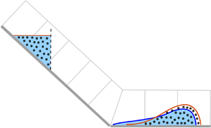
Figure 2. Schematic diagram showing the  $30^\circ$ inclined plane and the horizontal run-out pad in Taylor-Noonan et al.'s (Reference Taylor-Noonan, Bowman, McArdell, Kaitna, McElwaine and Take2022) experiments. A terrain following curvilinear coordinate system $oxyz$ is defined with the origin at the top of the inclined plane, the $x$-axis in the downslope direction, the $y$-axis across the slope and the $z$-axis being the upwards pointing normal. A Cartesian coordinate system $OXYZ$ is also defined with the origin $O$ at the slope transition, the $Z$-axis pointing in the opposite direction to gravity and the $X$-axis aligned with $x$. The initial saturated charge of grains and water lies in the region $x\in [x_t,x_f]$. Blue shading corresponds to water, while the grains occupy the region below the red free surface, which is partially filled with circular markers to denote the grains. During motion ( $t>0$), velocity shear results in the surface layer of (light grey coloured) grains migrating towards the front, whereas the (dark grey coloured) grains near the base are transported backwards relative to the advancing front. The inset diagram shows how the assumed shape of the initial charge is modified in the computations to account for the dilatation of the granular body as it begins to flow. The break in slope lies 6.73 m downslope of gate at $x=x_f$. The positions of the camera fields of view, ultrasonic height sensor and pressure transducer are illustrated on the main diagram. Movies 1 and 2 in the online supplementary material show typical dry and wet flow experiments.
Two different types of initial conditions were implemented in the experiments of Taylor-Noonan et al. (Reference Taylor-Noonan, Bowman, McArdell, Kaitna, McElwaine and Take2022). In the first, a series of five source volumes of dry monodisperse spherical ceramic beads with diameter  ${\sim }3.85$ mm were released on the chute. The source volumes started at 0.2 m $^3$ and incremented in 0.2 m $^3$ intervals until 1 m $^3$. In the second, identical volumes of water-saturated grains (of the same type used in the dry tests) were released to evaluate the effect of the pore fluid. These different initial conditions evolved into two dramatically different flow structures and deposit morphologies.
Figure 3 shows two typical high-speed camera images taken 6.23 m downstream of the gate and 0.5 m upstream of the slope break (see figure 2) for the dry and wet release volumes of  $V_{ini}=0.8$ m $^3$. In both cases there is an in-focus dense granular region adjacent to the wall, a few saltating grains above it and an out-of-focus perspective view of the free surface further away from the wall. In the case of the wet flow, there is also a well-defined phreatic surface adjacent to the wall, below which the grains are saturated. Taylor-Noonan et al. (Reference Taylor-Noonan, Bowman, McArdell, Kaitna, McElwaine and Take2022) used these high-speed images to determine the granular and phreatic free surfaces (adjacent to the wall), and showed them on a space–time plot formed from the high-speed camera images. Figure 4 shows the space–time plot of the high-speed images, and the granular and phreatic free surfaces, for the same experiment as figure 3. Note that the diffuse/blurred region above the granular free surfaces, is simply the way the out-of-focus grains (that are not adjacent to the wall) appear in these plots and has no influence on the results.

Figure 3. Taylor-Noonan et al.'s (Reference Taylor-Noonan, Bowman, McArdell, Kaitna, McElwaine and Take2022) high-speed movie images of the (a) dry and (b) wet flow experiments 0.5 m upstream of the slope break, 0.94 s after the initial front arrival and for initial volumes  $V_{ini}=0.8$ m $^3$. Movies 3 and 4 in the online supplementary material show the complete high-speed movie sequences, which are very instructive. All of Taylor-Noonan et al.'s (Reference Taylor-Noonan, Bowman, McArdell, Kaitna, McElwaine and Take2022) high-speed camera data is available from https://doi.org/10.5683/SP3/1ZCUFY.

Figure 4. Taylor-Noonan et al.'s (Reference Taylor-Noonan, Bowman, McArdell, Kaitna, McElwaine and Take2022) space–time plots measured 0.5 m above the slope break, for (a) dry and (b) water-saturated granular flows with an initial volume  $V_{ini}=0.8$ m $^3$. The dense flow adjacent to the glass sidewall is characterized by the black and white stippled region, while the diffuse/blurred region (above) corresponds to out-of-focus grains that are not adjacent to the sidewall, as well as to a few saltating grains. The red and blue lines are the grain and phreatic free surfaces determined from the individual high-speed images by Taylor-Noonan et al. (Reference Taylor-Noonan, Bowman, McArdell, Kaitna, McElwaine and Take2022) (see e.g. figure 3, where the interfaces are more clearly identifiable). In panel (a), the flow in the tail is quite dilute and the surface of the dense granular regime is difficult to define. The horizontal bands on the space–time plots are caused by dust, imperfections and water droplets on the sidewall of the chute, as can be seen in the online movies 3 and 4.
As mentioned above, the free surface positions of the grains and the water are determined from the individual high-speed images (e.g. figure 3) where most of the time they are clearly identifiable. The wet flows suppress grain saltation, compared with dry flows, which may dilate significantly if they are only a few particle diameters in thickness. This can lead to uncertainty in the position of the granular free surface in some of the smaller dry releases (Taylor-Noonan et al. Reference Taylor-Noonan, Bowman, McArdell, Kaitna, McElwaine and Take2022). In the main dense body of the dry flow (figure 4a) the thickness rises to a peak height of 5.5 cm approximately 1.2 s after the initial front arrival, and then the thickness decreases until approximately 3.1 s when an upslope propagating shockwave comes into view and partially brings the grains to rest. This can be seen in movie 3, which is available in the online supplementary material.
For the water-saturated flow, the flow head is almost completely dry as shown in figure 4(b) and movie 4. The grain peak height of 6.8 cm occurs only 0.5 s after the front arrival, and is significantly higher than that of the dry grains. The peak height of 4.3 cm for the phreatic (water) free surface occurs very slightly after that of the grains, implying that the flow front is undersaturated. The grain and phreatic free surfaces both decrease rapidly in height, while the wet flow remains undersaturated until approximately 3.4 s. After this time the tail becomes very watery and the water free surface is almost of constant height of 0.5 cm. Most of the wet flow is therefore in the undersaturated regime throughout the duration of the flow, except at the thin watery tail, which develops a series of roll waves.
During motion of the dry flow, Taylor-Noonan et al.'s (Reference Taylor-Noonan, Bowman, McArdell, Kaitna, McElwaine and Take2022) experiments (see their figure 9) show that the moving body of grains dilates from its static state. However, the dry experiments can still be modelled successfully without accounting for this dilation as shown in § 5. This dilation is particularly important for the flows of wet experiments, because it generates a mechanism of producing dry grains at the surface of the flowing material, which can then be sheared forwards and ultimately creates a drier more resistive flow front.
Movies 1 and 2 show that the water-saturated flow is much more mobile than the dry flow. For an initial volume of 0.8 m $^3$, the front of the wet flow extends $6.5$ m down the run-out pad from the break in slope, while the front of the dry flow only reaches $2.1$ m. The distal reach of the wet grains is therefore further than that of dry granular flows. Moreover, the experiments showed that the wet flow run-out distance grows with increasing source volume, while the barycentre of the dry deposits was almost identical for all five dry flow volumes. A Faro Focus S 150 light detection and ranging (LiDAR) scanner was used by Taylor-Noonan et al. (Reference Taylor-Noonan, Bowman, McArdell, Kaitna, McElwaine and Take2022) to detect the final deposit morphology for each of the release volumes. These detailed deposit profiles will be compared with the simulated wet and dry flows using Meng et al.'s (Reference Meng, Johnson and Gray2022) theory in §§ 5 and 6 of this paper.
3. Depth-averaged theory
Meng et al.'s (Reference Meng, Johnson and Gray2022) depth-averaged theory for granular-fluid flows is used in this paper to model the wet and dry experiments of Taylor-Noonan et al. (Reference Taylor-Noonan, Bowman, McArdell, Kaitna, McElwaine and Take2022). This requires the theory to be generalized to a terrain-following curvilinear coordinate system. In addition, since the experiments show that the flow is predominantly undersaturated, some simplifications can be made that make it easier to develop a numerical method.
3.1. Meng et al.'s depth-averaged equations
Let  $oxyz$ be a terrain-following curvilinear coordinate system with the $x$ axis pointing down the chute, the $y$-axis pointing across the slope and the $z$-axis being the upward pointing normal, as illustrated in figure 2. The origin $o$ is placed at the top of the chute upstream of the release gate and the local angle of inclination of the chute $\zeta =\zeta (x)$. In these coordinates the chute base lies along $z=0$. The chute geometry and the initial conditions are independent of $y$. Moreover, figure 1(a), and movies 1 and 2, show that the flow front remains planar across the chute, without forming significant boundary layers adjacent to the sidewalls. The sidewall friction and lateral gradients of physical quantities are therefore neglected, and the whole flow is modelled independently of $y$.
$y$.
In the curvilinear coordinate system the granular and phreatic (water) free surfaces lie at  $z=h^g$ and $h^w$, respectively. When $h^g>h^w$ the flow is undersaturated, while if $h^g< h^w$ the flow is oversaturated. These flow configurations are shown schematically in figure 2 of Meng et al. (Reference Meng, Johnson and Gray2022). In the undersaturated regime there is a layer of dry grains above a saturated mixture of grains and water, and the associated volume fractions of the grains and the water are
 \begin{equation} \phi^g=\phi^c, \quad
0\le z< h^g,\qquad \phi^w=\left\{\begin{array}{@{}ll} 0, &
h^w\le z< h^g,\\ 1-\phi^c, & 0\le z <
h^w,\end{array}\right.
\end{equation}
\begin{equation} \phi^g=\phi^c, \quad
0\le z< h^g,\qquad \phi^w=\left\{\begin{array}{@{}ll} 0, &
h^w\le z< h^g,\\ 1-\phi^c, & 0\le z <
h^w,\end{array}\right.
\end{equation}
respectively, where  $\phi ^c$ is constant (Iverson & Denlinger Reference Iverson and Denlinger2001). In the oversaturated regime, there is a layer of water on top of the saturated mixture of grains and water. The volume fractions of the grains and the water are therefore
 \begin{equation}
\phi^g=\left\{\begin{array}{@{}ll} 0, & h^g\le z< h^w,\\
\phi^c, & 0\le z < h^g, \end{array}\right.\quad
\phi^w=\left\{\begin{array}{@{}ll} 1, & h^g\le z< h^w,\\
1-\phi^c, & 0\le z < h^g. \end{array}\right.
\end{equation}
\begin{equation}
\phi^g=\left\{\begin{array}{@{}ll} 0, & h^g\le z< h^w,\\
\phi^c, & 0\le z < h^g, \end{array}\right.\quad
\phi^w=\left\{\begin{array}{@{}ll} 1, & h^g\le z< h^w,\\
1-\phi^c, & 0\le z < h^g. \end{array}\right.
\end{equation}
Note that the assumption that the volume fraction of the grains  $\phi ^g$ equals $\phi ^c$ wherever grains are present, implies that Meng et al.'s (Reference Meng, Johnson and Gray2022) theory cannot resolve excess pore pressure effects that occur due to changes in volume fraction. Nevertheless, this paper shows that Meng et al.'s (Reference Meng, Johnson and Gray2022) theory is sufficient to quantitatively capture the experiments of Taylor-Noonan et al. (Reference Taylor-Noonan, Bowman, McArdell, Kaitna, McElwaine and Take2022).
The grains and the water are assumed to be incompressible with constant intrinsic densities  $\varrho ^{g\star }$ and $\varrho ^{w\star }$, respectively. They also have independent velocity fields $\boldsymbol {u}^g=(u^g, w^g)$ and $\boldsymbol {u}^w=(u^w, w^w)$, where the components are measured in the downslope and normal directions. The depth-averaged velocities of the grains and the water, $\bar {u}^g$ and $\bar {u}^w$, in the downslope direction are defined as
 \begin{equation} \bar{u}^g=\frac{\displaystyle\int_{0}^{h^g}\phi^g u^g\,{\rm d}z}{\displaystyle\int_{0}^{h^g}\phi^g\,{\rm d}z}=\frac{\overline{\phi^g u^g}}{\bar\phi^g}, \quad \bar{u}^w=\frac{\displaystyle\int_{0}^{h^w}\phi^w u^w\,{\rm d}z}{\displaystyle\int_{0}^{h^w}\phi^w\,{\rm d}z}=\frac{\overline{\phi^w u^w}}{\bar\phi^w}, \end{equation}
respectively. Meng et al. (Reference Meng, Johnson and Gray2022) defined the proportion of the flow height that is occupied by grains in the undersaturated and oversaturated regimes as
 \begin{equation} \mathcal{H}=\left\{\begin{array}{@{}ll} 1, & h^g> h^w,\quad (\text{undersaturated}),\\ h^g/h^w, & h^g\le h^w, \quad (\text{oversaturated}), \end{array} \right. \end{equation}
which is useful in defining a unified system of equations (their equations (4.68)–(4.77)) that are valid in both the undersaturated and oversaturated regimes. In the undersaturated regime Meng et al.'s (Reference Meng, Johnson and Gray2022) equations can be written in conservative form, which is convenient for the development of numerical methods (Kurganov & Tadmor Reference Kurganov and Tadmor2000). However, in the oversaturated regime the equations cannot be written in conservative form, due to the buoyancy terms in their equations (4.72) and (4.73), which makes the construction of numerical methods more complex (Maso, LeFloch & Murat Reference Maso, LeFloch and Murat1995; LeVeque Reference LeVeque2002; Parés Reference Parés2006; Diaz, Kurganov & de Luna Reference Diaz, Kurganov and de Luna2019).
Since Taylor-Noonan et al.'s (Reference Taylor-Noonan, Bowman, McArdell, Kaitna, McElwaine and Take2022) experiments are predominantly in the undersaturated regime, this paper makes the minimal possible modification to the equations (in the oversaturated regime) in order to put them in conservative form. Specifically the modified depth-averaged grain and water mass and momentum balance equations are assumed to be
 $$\begin{gather} \frac{\partial}{\partial t}(h^g\phi^c) + \frac{\partial}{\partial x}(h^g\phi^c\bar{u}^g) = 0, \end{gather}$$
 $$\begin{gather}\frac{\partial}{\partial t}(h^g\phi^c\bar{u}^g) + \frac{\partial}{\partial x}(\chi^g h^g\phi^c(\bar{u}^g)^2)+\frac{\partial}{\partial x}\left(\frac{1}{2}(h^g)^2\phi^cg\cos\zeta\right)=\mathcal{L}^g, \end{gather}$$
 $$\begin{gather}\frac{\partial}{\partial t}(h^w\bar\phi^w) + \frac{\partial}{\partial x}(h^w\bar\phi^w \bar{u}^w) = 0, \end{gather}$$
 $$\begin{gather}\frac{\partial}{\partial t}(h^w\bar\phi^w\bar{u}^w) + \frac{\partial}{\partial x}(\chi^w h^w\bar\phi^w (\bar{u}^w)^2)+\frac{\partial}{\partial x}\left(\frac{1}{2}(h^w)^2\bar\phi^w g\cos\zeta\right)=\mathcal{L}^w, \end{gather}$$
respectively, where  $g$ is the constant of gravitational acceleration, $\mathcal {L}^g$ and $\mathcal {L}^w$ are source terms and $\bar \phi ^w$ is the depth-averaged water concentration. Using the assumed vertical water concentration distribution in the undersaturated and oversaturated regimes (3.1b)–(3.2b) as well as the definition (3.4) it follows that
 \begin{equation} \bar\phi^w=\frac{1}{h^w}\int_0^{h^w}\phi^w\,{\rm d}z=(1-\phi^c{\mathcal{H}}). \end{equation}
Equations (3.5)–(3.8) are identical to those of Meng et al. (Reference Meng, Johnson and Gray2022) in the undersaturated regime, while in the oversaturated regime the equations are asymptotically equivalent in the limit as the water thickness tends to the granular thickness from above, i.e.  $h^w\rightarrow h^{g+}$. Moreover, the form has been chosen so that when $h^g=0$, (3.7)–(3.8) reduce to the shallow water equations. In the convective momentum terms in (3.6) and (3.8), $\chi ^\nu =\overline {(u^\nu )^2}/(\bar {u}^\nu )^2$ is the shape factor and its value deviates from unity for sheared velocity profiles. For non-unity values of the shape factor, the characteristic structure of the depth-averaged system changes, and leads to the formation of a thin precursor layer ahead of the granular front, which is unphysical (Saingier, Deboeuf & Lagrée Reference Saingier, Deboeuf and Lagrée2016). Saingier et al. (Reference Saingier, Deboeuf and Lagrée2016) also showed that at low Froude numbers, non-unity values of the shape factor make very little difference to the overall shape of the granular flow front for $h>0$. This paper therefore assumes that $\chi ^\nu =1$ for both species $\nu =g,w$ for simplicity, in line with virtually all other debris-flow models (Pitman & Le Reference Pitman and Le2005; Pelanti et al. Reference Pelanti, Bouchut and Mangeney2008; Pudasaini Reference Pudasaini2012; Bouchut et al. Reference Bouchut, Fernadez-Nieto, Mangeney and Narbona-Reina2016; Meng & Wang Reference Meng and Wang2018).
Since the buoyancy terms in equations (4.72) and (4.73) of Meng et al. (Reference Meng, Johnson and Gray2022) have been subsumed into the modified momentum balances (3.6) and (3.8), it follows that the leading-order source terms for the grains and the water are
 $$\begin{gather} \mathcal{L}^g =\underbrace{h^g\phi^cg\sin\zeta}_{\textit{Gravity}}- \underbrace{\frac{\bar{u}^g}{\vert\bar{u}^g\vert}\left(1-\gamma\mathcal{H}\frac{ h^w}{h^g}\right) \mu^bh^g\phi^c(g\cos\zeta+\kappa(\bar{u}^g)^2)}_{\textit{Basal friction}} \nonumber\\ +\underbrace{\frac{C^d}{\varrho^{g\star}} (\psi^w(s)-\psi^g(s))}_{\textit{Darcy drag}}, \end{gather}$$
 $$\begin{gather}\mathcal{L}^w =\underbrace{h^w\bar\phi^w g\sin\zeta}_{\textit{Gravity}} -\underbrace{C^w\bar{u}^w\vert\bar{u}^w\vert}_{\textit{Basal friction}} -\underbrace{\frac{C^d}{\varrho^{w\star}} (\psi^w(s)-\psi^g(s))}_{\textit{Darcy drag}}, \end{gather}$$
where  $\gamma =\varrho ^{w\star }/\varrho ^{g\star }$ is the density ratio, $\mu ^b$ is a Coulomb-like basal friction coefficient for the grains and $\kappa =-\partial \zeta /\partial x$ is the curvature of the terrain-fitted coordinates, which modifies the basal pressure in the friction law (Savage & Hutter Reference Savage and Hutter1991; Gray et al. Reference Gray, Wieland and Hutter1999; Viroulet et al. Reference Viroulet, Baker, Edwards, Johnson, Gjaltema, Clavel and Gray2017). The water experiences a turbulent basal drag with the bed shear stress coefficient $C^w$, and the relative motion of the grains and the water within the mixture generates a Darcy drag, with Darcy drag coefficient $C^d$. The functional form of these coefficients, as well as the basal granular friction is discussed at greater length in § 3.2. The grain and water stream functions $\psi ^g$ and $\psi ^w$ in the Darcy drag terms are defined by
 \begin{equation} \psi^g(s)=\int_0^{s}u^g \,{\rm d}z, \quad \psi^w(s)=\int_0^{s}u^w \,{\rm d}z, \end{equation}
where the internal height of the saturated grain–water mixture
 \begin{equation} s = \begin{cases} h^w , & {h^g > h^w}, \quad (\text{undersaturated}),\\ h^g, & {h^g \le h^w}, \quad (\text{oversaturated}). \end{cases} \end{equation}
The stream functions allow the grain and water downslope velocity profiles with  $z$ to influence the relative motion of the two species. Specific profiles will be considered in § 3.3. It is these terms that are responsible for the deviation of Meng et al.'s (Reference Meng, Johnson and Gray2022) theory away from conventional debris-flow models that assume plug flow (Pitman & Le Reference Pitman and Le2005; Pelanti et al. Reference Pelanti, Bouchut and Mangeney2008; Iverson & George Reference Iverson and George2014; Bouchut et al. Reference Bouchut, Fernadez-Nieto, Mangeney and Narbona-Reina2016; Meng & Wang Reference Meng and Wang2016). Note that Meng et al.'s (Reference Meng, Johnson and Gray2022) depth-averaged viscous term for the water is neglected in (3.11), since it is not needed to model the experiments of Taylor-Noonan et al. (Reference Taylor-Noonan, Bowman, McArdell, Kaitna, McElwaine and Take2022). In addition, the use of the terrain-fitted coordinates implies that the basal topography gradient terms in equations (4.72) and (4.73) of Meng et al. (Reference Meng, Johnson and Gray2022) are zero, since $b=0$.
3.2. Granular friction, basal water drag and Darcy drag laws
Although the base of Taylor-Noonan et al.'s (Reference Taylor-Noonan, Bowman, McArdell, Kaitna, McElwaine and Take2022) chute is not roughened with particles, it is still rough enough that internal shear dominates over basal slip, as shown by the experimental peak flow velocity data in figure 5. It is therefore appropriate to apply the rough-bed basal friction law of Pouliquen & Forterre (Reference Pouliquen and Forterre2002), i.e.
 \begin{equation} \mu^b(Fr, h^g) = \mu_1 + \frac{\mu_2 - \mu_1}{1 + \displaystyle\dfrac{\beta h^g}{\mathscr{L}Fr}}, \end{equation}
where the Froude number  $Fr$ is defined as
 \begin{equation} Fr=\frac{\bar{u}^g}{\sqrt{g h^g\cos\zeta}}. \end{equation}
The rate-dependent friction law therefore starts at  $\mu _1=\tan \zeta _1$ at $Fr=0$ and asymptotes towards $\mu _2=\tan \zeta _2$ as $Fr/h^g$ tends towards infinity. The parameter $\beta$ is an empirical constant and $\mathscr {L}$ has the dimension of a length and is dependent on the properties of the particles and on the basal roughness. On a rough bed, the basal friction law (3.14) can be derived directly from the $\mu (I)$-rheology for granular flows (GDR-MiDi 2004; Jop, Forterre & Pouliquen Reference Jop, Forterre and Pouliquen2005; Gray & Edwards Reference Gray and Edwards2014). For flows on smoother slopes, Goujon, Thomas & Dalloz-Dubrujeaud (Reference Goujon, Thomas and Dalloz-Dubrujeaud2003) and Weinhart et al. (Reference Weinhart, Thornton, Luding and Bokhove2012) have shown that (3.14) still provides a good approximation for the friction, although the difference between $\zeta _2$ and $\zeta _1$ has to be reduced.

Figure 5. Non-dimensional downslope velocity profiles for the grains as a function of the non-dimensional depth, for the cubic ( $m=0.5$), Bagnold ( $m=2$) and linear shear with basal slip models ( $\alpha ^g=0.6$). The blue shaded region represents the $\pm 1$ standard deviation about the downslope velocity in Taylor-Noonan et al.'s (Reference Taylor-Noonan, Bowman, McArdell, Kaitna, McElwaine and Take2022) 0.8 m $^3$ experiment. The measurements are made in a 0.02 s observation time window during peak flow (their figure 6c) at 0.5 m above the slope break at approximately $t=2.05$ s.
The bed shear stress for the water phase takes account of the turbulent friction arising from the bottom of the channel. In the Meng et al. (Reference Meng, Johnson and Gray2022) paper,  $C^w$ was based on the Manning equation for open channel flows (Manning Reference Manning1891), and has the form
 \begin{equation} C^w=\bar\phi^w\frac{gn^2}{(h^w)^{{1}/{3}}}, \end{equation}
where  $n$ is the Manning coefficient (Chertock et al. Reference Chertock, Cui, Kurganov and Wu2015). The factor $\bar \phi ^w$ ensures that it reduces to the classical Chézy coefficient for water in the absence of grains. However, there are other empirical relations in the literature. The coefficient $C^w$ can also be related to the Darcy–Weisbach friction factor $f^{DW}$ as
 \begin{equation} C^w=\bar{\phi}^w\frac{f^{DW}}{8}, \end{equation}
where the factor  $\bar \phi ^w$ again ensures that in the absence of grains (3.17) reduces to the classical form of the pure water bed shear stress. A general and well-verified friction factor $f^{DW}$ is the White–Colebrook function corresponding to open channel flows (Silberman et al. Reference Silberman, Carter, Einstein, Hinds and Powell1963; Kleinhans Reference Kleinhans2005),
 \begin{equation} \sqrt{\frac{8}{f^{DW}}} = 5.74\log_{10}\left(\frac{h^w}{k_s}\right) + 6.24, \end{equation}
where  $k_s$ is Nikuradse roughness length commonly related to some grain size percentile of the mass frequency distribution. Since Taylor-Noonan et al. (Reference Taylor-Noonan, Bowman, McArdell, Kaitna, McElwaine and Take2022) experiments are monodisperse, the hydraulic roughness length is chosen to be equal to the grain diameter, i.e. $k_s=d$ (Kleinhans Reference Kleinhans2005). For the simulations shown in this paper, $C^W$ is assumed to obey the Manning equation (3.16). However, all of the computations have also been done with the Darcy–Weisbach formulation (3.17)–(3.18), and the results are virtually identical. The only difference appears to be in the tail of the flow, where the roll waves have a different amplitude and wavelength. The fact that the results are not sensitive to the precise formulation of $C^W$ suggests that the buoyancy reduced granular friction (3.10) dominates the response of the system.
The form of the Darcy drag coefficient is
 \begin{equation} C^d = \mu^w\frac{(1-\phi^c)^2}{k}, \end{equation}
where  $\mu ^w$ is the dynamic viscosity of water and the permeability $k = {(1-\phi ^c)^3d^2}/(180(\phi ^c)^2)$ is determined by Carman's formula for packing of spheres with diameter $d$ (Kozeny Reference Kozeny1927; Carman Reference Carman1937; Goharzadeh, Khalili & Jørgensen Reference Goharzadeh, Khalili and Jørgensen2005).
3.3. Assumed velocity profiles and associated stream functions
Vertical structure and velocity shear through the flow depth produce an important mechanism for differential species transport and the formation of large-rich and/or dry debris-flow fronts (Gray & Kokelaar Reference Gray and Kokelaar2010; Johnson et al. Reference Johnson, Kokelaar, Iverson, Logan, LaHusen and Gray2012; Baker et al. Reference Baker, Johnson and Gray2016; Gray Reference Gray2018; Viroulet et al. Reference Viroulet, Baker, Rocha, Johnson, Kokelaar and Gray2018). In Meng et al.'s (Reference Meng, Johnson and Gray2022) theory, shear-induced differential species transport is achieved by assuming downslope velocity profiles through the flow depth that deviate from plug flow.
In this paper three different granular velocity profiles are investigated that provide reasonable fits to Taylor-Noonan et al.'s (Reference Taylor-Noonan, Bowman, McArdell, Kaitna, McElwaine and Take2022) peak grain velocity data shown in figure 5. A general power-law downslope velocity, that satisfies the no-slip condition at the base and vanishing shear on the free surface, is given by
 \begin{equation} u^\nu(z) = \frac{1+2m}{1+m}\bar{u}^\nu\left[1-\left(1-\frac{z}{h^\nu}\right)^{({1+m})/{m}}\right], \end{equation}
where  $\nu =g,w$. This tends to a linear profile as the parameter $m\rightarrow \infty$ and tends to a plug profile as $m\rightarrow 0$ (Ng & Mei Reference Ng and Mei1994). The case $m=2$ corresponds to a Bagnold profile, which arises naturally from the $\mu (I)$ rheology for dry granular flows (GDR-MiDi 2004; Jop et al. Reference Jop, Forterre and Pouliquen2006; Gray & Edwards Reference Gray and Edwards2014). This is consistent with the assumed basal granular friction law (3.14), and provides a reasonable fit to the experimental velocity data for the grains shown in figure 5. A better fit is obtained for the case $m=0.5$, which corresponds to a cubic profile. Rather than this indicating a deviation away from the $\mu (I)$ rheology, the apparently better fit is likely due to the grains slipping somewhat on the smooth aluminium chute base. One can also simply assume a linear velocity profile with basal slip to characterize either the grains or water velocity field
 \begin{equation} u^\nu(z) = \bar{u}^\nu\left(\alpha^\nu + 2(1-\alpha^\nu)\frac{z}{h^\nu}\right), \end{equation}
where for  $\nu =g,w$ and the variable $\alpha ^\nu \in [0,1]$ controls the magnitude of the basal slip velocity (Gray & Thornton Reference Gray and Thornton2005; Gray & Ancey Reference Gray and Ancey2009). When $\alpha ^\nu =0$, (3.21) reduces to a linear profile with no slip at the base, and it reduces to plug flow, when $\alpha ^\nu =1$. For simplicity, the water is assumed to have a plug-flow profile, i.e. $u^w(z) = \bar {u}^w$.
The assumed grain and water velocity profiles enter Meng et al.'s (Reference Meng, Johnson and Gray2022) theory indirectly through the stream functions defined in (3.12). These are evaluated on the internal grain–water mixture surface  $s$ defined in (3.13). It follows that for the power law velocity profile (3.20), the stream function is
 \begin{equation} \psi^\nu(s)=\frac{m}{1+m}h^\nu\bar{u}^\nu\left[\frac{1+2m}{m}\left(\frac{s}{h^\nu}\right)-1+ \left(1-\frac{s}{h^\nu}\right)^{({1+2m})/{m}}\right], \end{equation}
and for the linear profile (3.21) it is
 \begin{equation} \psi^\nu(s)=h^\nu\bar{u}^\nu\left[\alpha^\nu\left(\frac{s}{h^\nu}\right)+(1-\alpha^\nu)\left(\frac{s}{h^\nu}\right)^2\right]. \end{equation}
For the assumed plug-flow water velocity field it follows that
 \begin{equation} \psi^w(s)=s\bar u^w. \end{equation}
The stream functions are used in the Darcy-drag terms in the momentum sources (3.10) and (3.11). These control the relative depth-averaged motion of the grains and the water in the water-saturated granular region at the base of the flow.
4. Numerical method and physical parameters
4.1. Numerical method
The system of conservation laws (3.5)–(3.8) is solved numerically using the shock-capturing non-oscillatory central scheme of Kurganov & Tadmor (Reference Kurganov and Tadmor2000). This robust scheme has been used to successfully solve a number of closely related systems of conservation laws for dry granular flows (Edwards & Gray Reference Edwards and Gray2015; Baker et al. Reference Baker, Johnson and Gray2016; Rocha, Johnson & Gray Reference Rocha, Johnson and Gray2019), debris flows (Meng et al. Reference Meng, Wang, Feng, Wang and Zhou2018, Reference Meng, Wang, Chiou and Zhou2020) and submarine landslides (Sun et al. Reference Sun, Meng, Wang, Hsiau and You2023). The method is a semidiscrete Riemann-free solver that maintains the non-oscillatory property by using a flux limiter. Here, the weighted essentially non-oscillatory limiter detailed in Noelle (Reference Noelle2000) is chosen, as in Baker et al. (Reference Baker, Johnson and Gray2016). The non-oscillatory central scheme requires the system of (3.5)–(3.8) to be written in a vector form
 \begin{equation} \frac{\partial\boldsymbol{U}}{\partial t} + \frac{\partial\boldsymbol{F}(\boldsymbol{U})}{\partial x} = \boldsymbol{S}(\boldsymbol{U}), \end{equation}
where the vector of conservative fields is defined as
 \begin{equation} \boldsymbol{U}=(H^g,M^g,H^w,M^w)^{\rm T}=(h^g\phi^c, h^g\phi^c\bar{u}^g, h^w\bar\phi^w, h^w\bar\phi^w\bar{u}^w)^\text{T}. \end{equation}
Three field variables are easy to express in terms of the conservative variables
 \begin{equation} h^g=\frac{H^g}{\phi^c},\quad \bar{u}^g=\frac{M^g}{H^g},\quad \bar{u}^w=\frac{M^w}{H^w}, \end{equation}
but the relation for  $h^w$ is dependent on whether the flow is undersaturated or oversaturated. Using the definition of $\bar \phi ^w$ in (3.9), it follows that
 \begin{equation} h^w = \begin{cases} \displaystyle\frac{H^w}{1-\phi^c}, & (\text{undersaturated}),\\ H^w+H^g, & (\text{oversaturated}), \end{cases} \end{equation}
and hence the depth-averaged water concentration is
 \begin{equation} \bar\phi^w = \begin{cases} {1-\phi^c}, & (1-\phi^c)H^g > \phi^c H^w,\quad (\text{undersaturated}),\\ \displaystyle\frac{H^w}{H^w+H^g}, & (1-\phi^c)H^g \le \phi^c H^w,\quad (\text{oversaturated}). \end{cases} \end{equation}
In the undersaturated regime the flux vector  $\boldsymbol {F}$ is
 \begin{equation} \boldsymbol{F}(\boldsymbol{U})= \left( \begin{array}{@{}c@{}} M^g \\ \displaystyle\dfrac{(M^g)^2}{H^g} +\dfrac{1}{2}\dfrac{(H^g)^2}{\phi^c}g\cos\zeta\\*[10pt] M^w \\ \displaystyle\dfrac{(M^w)^2}{H^w} +\dfrac{1}{2}\dfrac{(H^w)^2}{1-\phi^c} g\cos\zeta \end{array} \right),\quad (1-\phi^c)H^g > \phi^c H^w, \end{equation}
while in the oversaturated regime it is
 \begin{equation} \boldsymbol{F}(\boldsymbol{U})= \left( \begin{array}{@{}c@{}} M^g \\ \displaystyle\dfrac{(M^g)^2}{H^g} +\dfrac{1}{2}\dfrac{(H^g)^2}{\phi^c}g\cos\zeta\\ M^w \\ \displaystyle\dfrac{(M^w)^2}{H^w} +\dfrac{1}{2}(H^w+H^g)H^w g\cos\zeta \end{array} \right),\quad (1-\phi^c)H^g \le \phi^c H^w. \end{equation}
The characteristic wave speeds  $\lambda _i$ ( $i=1,\ldots,4$) of the system in both the undersaturated and oversaturated regimes are evaluated in Appendix A. In the undersaturated regime the structure of the system uncouples to generate two shallow-water-type systems (for the grains and for the water) that are weakly coupled through the momentum source terms. In the oversaturated regime there is stronger coupling through the flux vector. The system of equations is non-strictly hyperbolic in both undersaturated and oversaturated regimes, with explicit characteristic wave speeds given by (A4) and (A7).
The source vector  $\boldsymbol {S}$ is
 \begin{equation} \boldsymbol{S}(\boldsymbol{U})= \left( \begin{array}{@{}c@{}} 0 \\ \mathcal{L}^g \\ 0 \\ \mathcal{L}^w \end{array} \right), \end{equation}
where  $\mathcal {L}^g$ and $\mathcal {L}^w$ are defined in (3.10) and (3.11), respectively. The appearance of the water basal friction term in the form $-(1-\phi ^c\mathcal {H})gn^2u^w\vert {u\vert }^w/(h^w)^{{1}/{3}}$ is a potential challenge to the discretization of the source vector $\boldsymbol {S}(\boldsymbol {U})$, as the underlying semidiscrete system becomes stiff when the water thickness $h^w$ is small. In this case, small numerical oscillations might cause negative values of water thickness, which in turn would make it impossible to evaluate the characteristic wave speeds $\lambda _{3,4}$ in (A4b) and (A7b). To prevent the appearance of the negative thickness, this paper adopts the correction strategy of Chertock et al. (Reference Chertock, Cui, Kurganov and Wu2015) to correct the slopes of the conservative variables for small thicknesses during the reconstruction. Additionally, the water velocity at the centres of the cells, required to compute the water basal friction term, is computed at cell $j$ using the desingularization formula
 \begin{equation} \bar{u}_j^w = \frac{2H_j^w {M^w_j}}{(H_j^w)^2+\max((H_j^w)^2,\alpha^2)}, \end{equation}
where  $\alpha =5\times 10^{-5}$ m. Equation (4.9) ensures that its influence on the water velocity is negligibly small for the thicknesses $h^w\ge 100\alpha /(1-\phi ^c)$, which are sufficiently small compared with the peak flow depth. Since Kurganov & Tadmor's (Reference Kurganov and Tadmor2000) semidiscrete approach is an explicit scheme, a small time step $\Delta t$ is needed to maintain stable computation. To avoid reducing the time step significantly and simultaneously preserve strong stability of the computation, a splitting technique is used to discretize the water and grain basal friction terms. This has proved to be effective in ensuring a stable computation without the expense of decreasing the time step significantly (see Liang & Marche Reference Liang and Marche2009). The time step $\Delta t$ is given by
 \begin{equation} \Delta t \le \frac{\Delta x}{\vert a\vert} CFL, \quad\text{where } a=\max\left\{\vert\lambda_{i}\vert\right\},\quad i=1,\ldots,4, \end{equation}
and the Courant–Friedrichs–Lewy number  $CFL=0.1$ is chosen.
4.2. Computational geometry and boundary conditions
The computational domain is 20 m in length and the gate is located at  $x_f={\rm \pi}$ m. In the experiments, the inclined plane is sharply connected to a horizontal plane. This causes the curvilinear coordinates $oxz$ to overlap for $z>0$ at the slope break. To avoid overlap in the flow thicknesses in the computations, a short smooth transition is therefore added between the inclined and horizontal planes. The inclination angle of the slope is
 \begin{equation} \zeta(x) = \begin{cases} \zeta_0, & {0\le x\le x_a},\\ \zeta_0\left(1-\displaystyle\frac{x-x_a}{x_b-x_a}\right), & {x_a < x < x_b},\\ 0^\circ, & {x \ge x_b}, \end{cases} \end{equation}
where  $\zeta _0=30^\circ$, $x_a=x_f+6.73$ m, $x_b=x_f+7.13$ m. These values are summarized in table 1. The inclined section therefore extends 6.73 m downstream of the gate and the smooth transition is $0.4$ m in length. The smooth transition is sufficiently small compared with the overall chute length that its influence on the debris-flows dynamics is small. The centrifugal forces induced by the change in curvature $\kappa =-\partial \zeta /\partial x$ does, however, change the basal pressures in the transition region. This is accounted for by the curvature term in the granular source terms (3.10). Free outflow conditions are specified at either end of the domain, but in most simulations no material reaches either boundary. The computation domain is discretized into 4667 grid points, implying $\Delta x=0.0042857$ m.
Table 1. Computational chute geometry and physical parameters used to simulate Taylor-Noonan et al.'s (Reference Taylor-Noonan, Bowman, McArdell, Kaitna, McElwaine and Take2022) debris-flow experiments.

4.3. Initial conditions for the dry simulations
Dry grains are initially packed in a triangular region behind a vertical gate at  $x=x_f$ and have a horizontal free surface. In the terrain-following curvilinear coordinates the initial height is therefore given by
 \begin{equation} h^g_{{ini}} = \begin{cases} \displaystyle (x_f-x)\cot\zeta_0, & { x_m \le x\le x_f},\\ \displaystyle (x-x_t)\tan\zeta_0, & {x_t < x < x_m},\\ \displaystyle 0, & \text{otherwise}, \end{cases} \end{equation}
where  $x_m$ is the downslope position of the maximum depth (measured normal to the plane) and $x_t$ is the maximum upstream position of the triangular pile. The initial grain volume $V_{{ini}}$ is uniformly distributed across the chute, which is of width $W=2.09$ m. The two-dimensional projected area can therefore be used to determine $x_t$ and $x_m$, which are given by the expressions
 \begin{equation} x_t=x_f - \sqrt{\frac{2V_{ini}}{W\sin\zeta_0\cos\zeta_0}}, \quad x_m=x_f - (\tan\zeta_0)\sqrt{\frac{2V_{{ini}}\sin\zeta_0\cos\zeta_0}{W}}, \end{equation}
respectively. Computations for the dry granular flows assume that  $h^w=0$ and $C^w=0$, which implies that the depth-averaged water mass and momentum balances (3.7)–(3.8) are trivially satisfied. The depth-averaged granular mass and momentum balances (3.5)–(3.6) then reduce to those of Viroulet et al. (Reference Viroulet, Baker, Edwards, Johnson, Gjaltema, Clavel and Gray2017).
4.4. Initial conditions for wet simulations
In the wet flow experiments the initial volume of grains held behind the gate is in exactly the same configuration as the dry grains in § 4.3, and occupies a total volume  $V_{ini}$. The only difference is that the interstices between the grains are now occupied by water rather than air. Since the grains are initially saturated, the intrinsic volumes of grains and water (i.e. the volumes of the pure phases) are therefore
 \begin{equation} V^{g\star}_{ini}=V_{ini}\phi^g_{ini}, \quad V^{w\star}_{ini}=V_{ini}(1-\phi^g_{ini}), \end{equation}
where  $\phi ^g_{ini}$ is the granular volume fraction in the initial deposit.
Meng et al.'s (Reference Meng, Johnson and Gray2022) theory uses a constant solids volume fraction  $\phi ^g=\bar \phi ^g=\phi ^c$ that does not change during flow. The only way to model the initial dilatation of the granular matrix, observed in the Taylor-Noonan et al.'s (Reference Taylor-Noonan, Bowman, McArdell, Kaitna, McElwaine and Take2022)'s experiments, is therefore to change the assumed initial configuration to account for the subsequent change in $\phi ^g$ from $\phi ^g_{ini}=0.585$ to $\phi ^c=0.48$. For the grains, this is done by expanding the initial height, to account for the solids volume fraction, without changing the initial $x$ position, i.e.
 \begin{equation} h^g_{new}=\frac{\phi^g_{ini}}{\phi^c}h^g_{ini}, \end{equation}
where  $h^g_{ini}(x)$ is defined in the same way as the initial dry height (4.13). In particular, the maximum height, which is still attained at $x=x_m$, is now
 \begin{equation} h^g_{max}=\frac{\phi^g_{ini}}{\phi^c}(x_f-x_m)\cot\zeta_0. \end{equation}
This expansion of the granular body in the normal direction to the chute, changes the assumed angle between the gate and the bed to
 \begin{equation} \theta = \arctan\left( \frac{h^g_{max}}{x_f-x_m} \right)=\arctan\left( \frac{\phi^g_{ini}}{\phi^c}\cot\zeta_0 \right), \end{equation}
as shown in the inset diagram in figure 2. This modifies the gate angle from  $60^\circ$ in the dry case, to $\theta =63.67^\circ$ in the wet case, independently of the initial volume.
The total volume of the water  $V^{w\star }_{ini}$ is also conserved, but it now occupies a smaller projected area in the $xz$ plane, because there is more pore space between the grains. For simplicity, it is assumed that the water remains in contact with the gate and occupies a triangular region defined by
 \begin{equation} h^w_{{ini}} = \begin{cases} \displaystyle h^w_{max}(x_f-x)/(x_f-x_w), & { x_w \le x\le x_f},\\ \displaystyle h^w_{max}(x-x_t)/(x_w-x_t), & {x_t < x < x_w},\\ \displaystyle 0, & \text{otherwise}, \end{cases} \end{equation}
where  $x=x_w$ is the downslope position of the maximum water height $h^w_{max}$. Accounting for the dilatation of the grain matrix, conservation of $V_{ini}^{w\star }$ implies
 \begin{equation} h^w_{max}=\left(\frac{1-\phi^g_{ini}}{1-\phi^c}\right)(x_f-x_m)\cot\zeta_0. \end{equation}
This implies that in curvilinear coordinates the maximum initial height of the water lies at
 \begin{equation} x_w= x_f - h^w_{max}\cot\theta. \end{equation}
As can be seen in the inset of figure 2, the net effect of these modifications is to produce an initially saturated flow front that transitions to an undersaturated region in the tail, where the peak height occurs (in terrain-following coordinates).
4.5. Physical parameters used in the simulations
Taylor-Noonan et al. (Reference Taylor-Noonan, Bowman, McArdell, Kaitna, McElwaine and Take2022) provided the values of the slope angle  $\zeta _0$, the grain and water densities $\varrho ^{g\star }$ and $\varrho ^{w\star }$, the grain diameter $d$ and the water viscosity $\mu ^w$. The base of the inclined plane is made of bare aluminium and therefore this paper assumes Manning's coefficient $n=0.016\ \text {s}\ \text {m}^{-1/3}$, which is within the commonly used range (see Chow Reference Chow1959). In the current theory, the solids volume fraction $\phi ^c$ is assumed to be constant; however, it varies with time and space in the experimental flows, as discussed in § 4.4. Taylor-Noonan et al.'s (Reference Taylor-Noonan, Bowman, McArdell, Kaitna, McElwaine and Take2022) wet experiment data (in their figure 9) suggests that $\phi ^c=0.48$ is a good approximate mean value. The initial solids volume fraction of $\phi ^g_{ini}=0.585$ is that of a very loose random packing. These experimental parameters and computational choices are summarized in table 1.
In addition, it is necessary to provide values of the parameters in the dynamic basal friction law (3.14) for the grains. The grains are of mean diameter  $d=3.85$ mm. With such large grains direct measurements of the friction angles are difficult to obtain, because it is not easy to carry out the tilting table experiments to determine $h_{stop}(\zeta )$ as in Pouliquen & Forterre (Reference Pouliquen and Forterre2002). This paper therefore adopts the same values of $\mathscr {L}=1.65\times d$ and $\beta =0.135$ used by Meng et al. (Reference Meng, Johnson and Gray2022) to match Davies's (Reference Davies1988, Reference Davies1990) moving-bed-flume experiments with polyvinyl chloride (PVC) cut rod on a toothed belt.
To provide insights into the choice of angles  $\zeta _1$ and $\zeta _2$, the parameters corresponding to the glass beads presented in Pouliquen (Reference Pouliquen1999) and the PVC rod presented in Meng et al. (Reference Meng, Johnson and Gray2022) are first used to conduct a series of dry flow calibration simulations. These are compared with the deposit in Taylor-Noonan et al.'s (Reference Taylor-Noonan, Bowman, McArdell, Kaitna, McElwaine and Take2022) experiment with an initial 0.8 m $^3$ volume of dry grains. Figure 6 shows that simulations with the PVC rod leave a significant deposit on the chute. This implies that $h_{stop}(\zeta _0)>0$ when $\zeta _2>\zeta _0$. This is not the case in the experiments, and hence the maximum friction angle $\zeta _2$ should be smaller than the slope angle $\zeta _0$. The simulations for glass beads show that the avalanche front, avalanche tail and the centre of mass of the deposit all lie too far upstream compared with Taylor-Noonan et al.'s (Reference Taylor-Noonan, Bowman, McArdell, Kaitna, McElwaine and Take2022) measured deposit. This is an indication that on average the friction is too high for the ceramic particles on the smooth aluminium bed. A good fit to Taylor-Noonan et al.'s (Reference Taylor-Noonan, Bowman, McArdell, Kaitna, McElwaine and Take2022) deposit is obtained by decreasing the value of $\zeta _2$ and increasing the value of $\zeta _1$ as shown in figure 6. All the computational results in the rest of this paper use the same frictional parameters, which are given in the last row of table 2.

Figure 6. Comparison between experimentally measured deposit morphology (red dash line) and theoretical predictions using the parameters for PVC rod (blue dotted line with the symbol ‘ $\star$’), for glass beads (blue dash–dot line with the symbol ‘ ${\square }$’) and the parameters used in the paper (red solid line). The parameters are summarized in table 2. This plot is made using the Cartesian coordinate system $OXZ$ shown in figure 2.
Table 2. Material properties for (a) glass beads (Pouliquen Reference Pouliquen1999), (b) PVC rod on a rough bed (Davies Reference Davies1990; Meng et al. Reference Meng, Johnson and Gray2022) and (c) the present choice of parameters for Taylor-Noonan et al.'s (Reference Taylor-Noonan, Bowman, McArdell, Kaitna, McElwaine and Take2022) experiments with approximately spherical rough ceramic beads on a smooth aluminium chute.

5. Dry simulations
Figure 7 and movie 5 show the simulated temporal and spatial evolution of the dry granular free surface after a 0.8 m $^3$ volume release. The mass accelerates downslope due to gravity and spreads rapidly due to the gradients of the depth-averaged internal pressure (the third term of the left-hand side of (3.6)). These pressure gradients result in the tail of the avalanche remaining stationary until approximately $2$ s. At $t=1.69$ s the flow front reaches the horizontal run-out plane, where the $g\sin \zeta$ component of the gravitational acceleration becomes zero. Basal granular friction then rapidly brings the front to rest by $t=2.6$ s. Meanwhile, the main body of grains is still accelerating down the chute. For $t>2.6$ s, these grains impact the frontal deposit, causing a shockwave to form (a rapid change in the flow thickness and velocity), which propagates upstream. This brings the oncoming flow rapidly to rest and builds up a thick deposit (Savage & Hutter Reference Savage and Hutter1991; Gray et al. Reference Gray, Tai and Noelle2003; Viroulet et al. Reference Viroulet, Baker, Rocha, Johnson, Kokelaar and Gray2018). By $t=6.76$ s the entire flow has been brought to rest and forms a compact static deposit that is largely contained in the region $x\in [10,12]$ m, and whose centroid is located at $x\simeq 11$ m.

Figure 7. Simulated temporal and spatial evolution of the granular free surface after 0.8 m $^3$ of grains are released from the flume gate. Since the flow height is very small compared with the chute length, the flow thickness is multiplied by a factor of four and projected normally to the chute along the straight grey lines to aid visualization. An animation is included in the online supplementary material (movie 5). Note that the view has been chosen to allow direct comparison with the wet simulations in §§ 6 and 7.
The simulated flow dynamics is similar to that observed in experiments, and shown in movie 1 for a  $0.8$ m $^3$ release. In fact, Taylor-Noonan et al. (Reference Taylor-Noonan, Bowman, McArdell, Kaitna, McElwaine and Take2022) released five different initial volumes ranging from 0.2 to 1 m $^3$. Quantitative comparisons of the simulations with Taylor-Noonan et al.'s (Reference Taylor-Noonan, Bowman, McArdell, Kaitna, McElwaine and Take2022) LiDAR measurements of the deposit heights are shown in figure 8. The parameters $\zeta _1$ and $\zeta _2$ were chosen in § 4.5 to match the $V_{{ini}}=0.8$ m $^3$ deposit shown in figure 8(d). Figure 8 shows that using the same parameters, all the computed deposits are in close agreement with the morphology seen in the experiments. In particular, the results capture Taylor-Noonan et al.'s (Reference Taylor-Noonan, Bowman, McArdell, Kaitna, McElwaine and Take2022) experimental observation that the position of the centre of mass of each deposit lies at approximately the same position, independently of the initial volume. This is despite the fact that the $V_{{ini}}=0.2$ and $0.4$ m $^3$ experiments become dilute during the flow. The ability of the dry model to capture both the centre of mass position and the spread of the deposit for all the initial release volumes provides independent verification that the selected parameters are good ones.

Figure 8. Comparison of the predicted deposit morphology (solid red line) and that measured in Taylor-Noonan et al.'s (Reference Taylor-Noonan, Bowman, McArdell, Kaitna, McElwaine and Take2022) experiments (red dashed line) for a release of (a) 0.2, (b) 0.4, (c) 0.6, (d) 0.8 and (e) 1.0 m $^3$ of dry granular material. Black lines represent the basal terrain and black ‘ $\star$’ symbols mark the start and end of the smooth transition. Black ‘ $\circ$’ and red ‘ $\star$’ represent barycentres of the experimental and predicted deposit, respectively. All the results are plotted in $OXZ$ coordinates. Note that the view has been chosen to allow direct comparison with the wet simulations in §§ 6 and 7.
6. Wet flow simulations assuming a cubic velocity profile
6.1. Temporal and spatial evolution of an 0.8 m $^3$ saturated release

The simulated temporal and spatial evolution of the release of 0.8 m $^3$ of initially water saturated grains is shown in figure 9. As detailed in § 4.4, the dilation of the granular matrix on failure (and hence the dilated grain matrix during flow) are modelled by adjusting the initial granular and water heights to account for the dilatation. This results in the front of the flow being initially saturated, and the tail of the flow being undersaturated at $t=0^+$ (see the inset in figure 2). The initial collapse looks similar to that of the dry grains ( $t\simeq 1$ s). However, the presence of the water in the main body of the flow reduces the basal granular friction in the source term (3.10), allowing the whole body to spread out faster than the purely dry flow. The tail of the grains therefore starts to move from its initial position by $t\simeq 1.82$ s.

Figure 9. Simulated spatial and temporal evolution of the grain and phreatic free surfaces after the 0.8 m $^3$ of water-saturated grains are released from the flume gate. The simulations assume the cubic velocity profile (3.20) with $m=0.5$, and the water has a plug-flow profile. Since the flow height is very small compared with the chute length, the flow thickness is multiplied by a factor of four and projected normally to the chute along the straight grey lines to aid visualization. An animation is included in the online supplementary material (movie 6). The inset depicts the roll waves developed in the tails at $t=5$ s in the range $x\in [8.26, 9.42]$ m and indicated by the dashed box.
By  $t=1$ s a dry front has already formed. Small dry fronts can form in plug-flow simulations due to mobility differences between the grains and the fluid, as will be shown in § 7.1. Here, a cubic velocity profile (3.20) is assumed, and the increased size of the dry front is due to the combination of vertical structure and velocity shear. This allows the undersaturated flowing layer of dry grains near the free surface to be rapidly transported to the front, even though it started at the back of the initial release volume.
On the inclined section, the dry granular front is able to grow in size because dry grains are being continually supplied by velocity shear, and because the internal water front experiences high resistance. This increased resistance is due to the water friction term in (3.11) remaining finite as  $h^w\rightarrow 0$, whereas all the other terms in the water momentum balance (3.8) tend to zero, i.e. the water friction generates singular behaviour. As the flow stretches out and the water layer becomes progressively thinner it experiences more basal resistance. In order to overcome this, an infinite gradient has to form at the water front for it to move.
The whole mixture accelerates more rapidly downslope than the purely dry flow. Indeed by  $t=1.5$ s, the dry front has already reached the horizontal run-out plane, where it decelerates and tries to stop. It does not fully come to rest, but is pushed along by the pressure exerted by the continued supply of high-speed, low-friction undersaturated material from upstream. The dry front impedes the flow, and a bulbous head forms that is analogous to that developed in bidisperse particle flows (Denissen et al. Reference Denissen, Weinhart, Voortwis, Luding, Gray and Thornton2019). At the transition between the thinner more mobile upstream region and the thicker more slowly moving head, a shockwave forms. The shock is smaller than the purely dry case and does not immediately start travelling upstream. Instead, for $1.69\le t\le 3.64$ s the shock travels downslope at a slightly slower speed than both the granular and water fronts, which move downstream approximately in unison. For times $t\in [3.64,4.16]$ s, the shock briefly propagates a short distance upstream, before dissipating. During the whole of this time $t\in [1.69, 4.016]$ s the thicker undersaturated head region grows in size. The fact that granular and water fronts move at the same speed (at least for a brief period of time), suggests that the flow front is similar to the first type of travelling wave solutions found by Meng et al. (Reference Meng, Johnson and Gray2022). Meanwhile, in the tail, the grains experience less basal friction than the water, and they are able to flow faster downslope to leave a thin oversaturated region on the chute that takes a very long time to drain down.
At  $t\simeq 4.29$ s, the granular front essentially stops, and there is some residual slow water percolation through the grains. A diffuse wave then travels upslope and almost all the grains come to rest by $t=6.24$ s. In the tail, the flow goes unstable and a close-up view shows that a series of roll waves form (see inset plot in figure 9). Similar waves can also be seen in the wet experiments in movie 2. At approximately $t=8$ s the grains are completely deposited on the horizontal run-out plane and the pore water drains slowly out of the granular matrix.
6.2. Comparison with Taylor-Noonan et al.'s (Reference Taylor-Noonan, Bowman, McArdell, Kaitna, McElwaine and Take2022) experimental time series
Taylor-Noonan et al. (Reference Taylor-Noonan, Bowman, McArdell, Kaitna, McElwaine and Take2022) photographed the flow with a high-speed camera that was located 0.5 m upstream of the slope break at  $x=x_f+6.23$ m. They used these images to determine the approximate position of the granular and phreatic (water) free surfaces as a function of time (see also, e.g. figures 3 and 4). Taylor-Noonan et al.'s (Reference Taylor-Noonan, Bowman, McArdell, Kaitna, McElwaine and Take2022) experimental results are now compared with the simulated time series for each of the release volumes in figure 10(a–e). All the simulated flow profiles show that there is an initially dry front, that is followed by an undersaturated flow with a peak height that occurs within the first second after the initial front arrival. The arrival time of the wet front is broadly in line with that observed in experiment, although some of the fronts are highly undersaturated, but not completely dry. The main body of the flow travels past the camera within the first two seconds, when the flow is travelling very quickly. The peak height increases with increasing initial release volume, with the granular peak height occurring slightly before the phreatic peak height in all cases. Two seconds after the initial front arrival, all the flows are much thinner and slower, and there is a gradual transition to the oversaturated regime, where roll waves form both in the experiments and the numerical simulations. The simulated time series for the granular and phreatic free surfaces are in good quantitative agreement with measurement. This is remarkable, given that the basal granular friction law was calibrated by matching the deposit position of a single dry experiment. The results are also in broad qualitative agreement with some debris-flow types observed in the field (McArdell et al. Reference McArdell, Bartelt and Kowalski2007; Nagl, Hübl & Kaitna Reference Nagl, Hübl and Kaitna2020).

Figure 10. Comparison of the predicted and measured time-series of the flow depths at  $x=x_f+6.23$ m for both (a–e) wet and (f–j) dry granular flows with source volumes of (a,f) 0.2, (b,g) 0.4, (c,h) 0.6, (d,i) 0.8 and (e,j) 1.0 m $^3$. The dashed red and blue lines show the experimental granular and phreatic (water) free surfaces determined by Taylor-Noonan et al. (Reference Taylor-Noonan, Bowman, McArdell, Kaitna, McElwaine and Take2022). The solid red line shows the grain thickness and the grey hashing shows the region occupied by grains. The blue solid line shows the position of the phreatic free surface, and the region beneath it is shaded blue to help visualize the water-saturated region. Taylor-Noonan et al.'s (Reference Taylor-Noonan, Bowman, McArdell, Kaitna, McElwaine and Take2022) high-speed camera data is available from https://doi.org/10.5683/SP3/1ZCUFY.
It is also interesting to compare the wet results with the equivalent time series for dry flows. These are shown in figure 10(f–j). For the smaller initial volumes  $V_{ini}=0.2$ and $0.4$ m $^3$, high-speed images in Taylor-Noonan et al.'s (Reference Taylor-Noonan, Bowman, McArdell, Kaitna, McElwaine and Take2022) supplementary material show that the dry flows become dilute. This makes determining the free surface more difficult, and since the flow is expanded, the discrepancy between the theoretical and measured free-surface heights is significant. As the source volume of the dry flows increases, however, a larger portion of the flow depth exceeds 10 particle diameters and the grains behave more like a dense flow. The comparisons for the larger initial dry granular volumes are therefore very good. For all the volumes, the computed dry flows are slower than the wet flows, which leads to a wider time series, with a lower peak height, than the wet flows. In addition, roll waves do not emerge in the tail of the dry flows, which is also captured by the theory. For $V_{ini}= 0.8$ and $1.0$ m $^3$, the upslope propagating shockwaves (which deposit the grains) come into the camera field of view, and the data after approximately three seconds is cut (Taylor-Noonan et al. Reference Taylor-Noonan, Bowman, McArdell, Kaitna, McElwaine and Take2022). For the wet flows, it is evident that the fluid viscosity suppresses most of the saltation (regardless of the initial release volume), so the theoretical and experimental comparisons are better than for the dry flows.
6.3. Comparison with Taylor-Noonan et al.'s (Reference Taylor-Noonan, Bowman, McArdell, Kaitna, McElwaine and Take2022) final deposits
A LiDAR scanner was used to determine the deposit height of the grains after the water had fully drained out (at least a day after the experiment). In this final configuration the grains have a denser packing than during flow when shear induces dilation. In order to compare the simulations with the experimental data it is necessary to now contract the granular matrix. At each location the depth of the grains is therefore adjusted to account for the increase in solids volume fraction from its flowing value  $\phi ^c$ to its deposited value, which is assumed to be the same initial solids volume fraction $\phi ^g_{{ini}}$,
 \begin{equation} h^g_{{dep}} = \left(\frac{\phi^c}{\phi^g_{{ini}}}\right) h^g. \end{equation}
The water height is then adjusted to conserve mass
 \begin{equation} h^w_{{dep}} = \begin{cases} \displaystyle\left(\frac{1-\phi^c}{1-\phi^g_{{ini}}}\right) h^w, & {h^g > h^w}, \\ h^w, & {h^g \le h^w}. \end{cases} \end{equation}
 Figure 11 shows a comparison between the deposit thickness adjusted for the increase in volume and Taylor-Noonan et al.'s (Reference Taylor-Noonan, Bowman, McArdell, Kaitna, McElwaine and Take2022) measured deposit thickness for the five wet release volumes. As has been seen in the simulations of the 0.8 m $^3$ case (figure 9), the dry front tries to stop when it reaches the horizontal plane, but the high-mobility undersaturated flow behind pushes the front forwards. As a result the wet flow deposits all show markedly increased run-out distances compared with the dry deposits (figure 8). The larger wet releases go further than the smaller wet ones, which contrasts with the dry case, where the deposit centre of masses were all approximately at $X\simeq 1$ m. Also, rather than forming a large heap at the bottom of the chute, the wet deposits are thinner and spread out along the run-out pad. The thickest part of the deposit is in the vicinity of the front. Here there is a flat-topped deposit that is thicker and longer for the larger release volumes. The simulated deposit then connects to a thinner upstream section that did not pass through the shock that forms during the deposition process, shown in figure 9 and movie 6. The simulation and experimental deposits are in very good agreement with each other, both in terms of their overall morphology, their front positions and thicknesses. There are, however, some differences. The experimental deposits do not show evidence of a shockwave having formed, and so have a much more gradual transition between the thick frontal section and the thinner tail. This may be an indication that the viscosity of the granular material is able to diffuse the shock (Gray & Edwards Reference Gray and Edwards2014). In addition, a thin layer of granular material remains on the chute in the experiments, but the computations show that all the grains drain off. This may be an indication that the assumed friction in the tail is too low in the simulations.

Figure 11. Comparison of the simulated granular free surface adjusted for the decrease in volume (red solid line) with the experimental free surface (red dashed line) for initial release volumes of (a) 0.2, (b) 0.4, (c) 0.6, (d) 0.8 and (e) 1.0 m $^3$ of water-saturated grains (Taylor-Noonan et al. Reference Taylor-Noonan, Bowman, McArdell, Kaitna, McElwaine and Take2022). The predicted profiles assume a cubic velocity profile during flow and are taken at $t=8$ s when the grains (grey hashed region) have stopped moving and the pore water (blue shaded region) is draining out of the matrix. The black lines are the basal terrain, and the ‘ $\star$’ symbols mark the start and end of the smooth transition.
7. Wet flow simulations for different velocity profiles
7.1. Wet flow simulations assuming plug flow
The model in this paper differs from traditional debris-flow models by its inclusion of vertical flow structure and velocity shear, which provide an important mechanism for the differential transport of the water and the grains (Meng et al. Reference Meng, Johnson and Gray2022). In contrast, traditional debris-flow models usually assume plug flow of both the grains and the water through the depth of the flow, i.e.
 \begin{equation} u^g = \bar{u}^g,\quad u^w = \bar{u}^w, \end{equation}
(Iverson & Denlinger Reference Iverson and Denlinger2001; Pitman & Le Reference Pitman and Le2005; Pelanti et al. Reference Pelanti, Bouchut and Mangeney2008; Pudasaini Reference Pudasaini2012; Iverson & George Reference Iverson and George2014; Bouchut et al. Reference Bouchut, Fernadez-Nieto, Mangeney and Narbona-Reina2016; Meng & Wang Reference Meng and Wang2018). In order to quantify the difference between the two approaches it is useful to solve the current model with the plug flow assumption (7.1). It follows from (3.12) that the grain and water stream functions are
 \begin{equation} \psi^g(s) = s\bar{u}^g, \quad \psi^w(s) = s\bar{u}^w, \end{equation}
where recall that  $s$ is defined as the height of the saturated grain–water layer in (3.13). These stream functions modify the Darcy drags in the source terms (3.10) and (3.11), and hence change the relative mobility of the grains and the water.
Figure 12 shows the computed temporal and spatial evolution of a 0.8 m $^3$ release of water-saturated grains assuming plug flow. Just as in the cubic velocity case, shown in figure 9, the initial release rapidly spreads out as it flows down the chute, and the flow front reaches the run-out pad at an almost identical time of $t=1.5$ s. The subtle difference is that the flow front only has a very small dry region. Since shear-induced transport has been eliminated in these simulations, the dry front that forms is purely due to the fact that the grains are more mobile than the water near the flow front. This mobility difference is a direct consequence of the degenerate nature of the basal friction law for the water, which requires an infinite gradient to form at the water front for it to propagate downslope. This mobility-induced relative motion of the water and grains near the front also implies that immediately behind the flow front the material is oversaturated (at $t=1.5$ s). This is not observed in Taylor-Noonan et al.'s (Reference Taylor-Noonan, Bowman, McArdell, Kaitna, McElwaine and Take2022) time series in figure 10(d), where the phreatic surface is below the grain surface in the vicinity of the front. In addition, now that shear-induced transport has been eliminated, the dry grains in the initially undersaturated region in the release (figure 2) cannot migrate forwards. The tail of the flow therefore remains undersaturated and does not develop roll waves, which also contradicts Taylor-Noonan et al.'s (Reference Taylor-Noonan, Bowman, McArdell, Kaitna, McElwaine and Take2022) observations.

Figure 12. Simulated spatial and temporal evolution of the grain and phreatic free surfaces when 0.8 m $^3$ of water-saturated grains is released from behind the flume gate. Both the grains and the water are assumed to have the plug-flow velocity profiles defined in (7.1). Since the flow height is very small compared with the chute length, the flow thickness is multiplied by a factor of four and projected normally to the chute along the straight grey lines to aid visualization. An animation is included in the online supplementary material (movie 7).
Although the small region of dry grains at the front may look like a small difference at  $t=1.5$ s to the simulations in figure 9, it has a profound effect on the subsequent flow on the horizontal run-out pad. The increased amount of water close to the front dramatically increases its mobility, so it is easier to push it forwards. As a result, when the grains finally stop at approximately $t=7$ s the front lies at slightly over 18 m. This contrasts with a run out of approximately $16.4$ m when velocity shear is included (as seen in figure 9). Figure 13 shows that all the initial release volumes lead to extended run-out behaviour with the plug-flow assumption. Making a plug-flow assumption in debris-flow models may therefore lead to enhanced run-out predictions, dramatically different local flow compositions and the suppression of roll waves.

Figure 13. Comparison of the simulated granular free surface adjusted for the decrease in volume (red solid line) with the experimental free surface (red dashed line) for initial release volumes of (a) 0.2, (b) 0.4, (c) 0.6, (d) 0.8 and (e) 1.0 m $^3$ of water-saturated grains (Taylor-Noonan et al. Reference Taylor-Noonan, Bowman, McArdell, Kaitna, McElwaine and Take2022). The predicted profiles assume plug flow and are taken at $t=8$ s when the grains (grey hashed region) have stopped moving and the pore water (blue shaded region) is draining out of the matrix. The black lines are the basal terrain, and the ‘ $\star$’ symbols mark the start and end of the smooth transition.
7.2. Influence of the assumed velocity profile on the final deposit morphology
The numerical simulations in § 7.1 of this paper showed that the run-out distance was overpredicted when plug-flow velocity profiles were assumed for the grains and the water. In contrast, the simulations in § 6 show that Meng et al.'s (Reference Meng, Johnson and Gray2022) model is able to make good quantitative predictions for the position of the Taylor-Noonan et al.'s (Reference Taylor-Noonan, Bowman, McArdell, Kaitna, McElwaine and Take2022) deposit, when a cubic granular velocity profile is assumed. Figure 5 shows that there is quite a bit of scatter in Taylor-Noonan et al.'s (Reference Taylor-Noonan, Bowman, McArdell, Kaitna, McElwaine and Take2022) peak-flow velocity data. A variety of functional forms could have been chosen to fit it. One may therefore legitimately ask how sensitive are the latter results to the precise parameterization of the velocity profile?
Figure 14 shows a comparison of the computed deposits for plug-flow (figure 14a), cubic (figure 14b), Bagnold (figure 14c) and linear profile with basal slip (figure 14d), velocity profiles, using the fitting parameters from § 3.3. The results in figure 14(b–d) use shear profiles that are broadly in agreement with one another, and all of them provide a good fit to Taylor-Noonan et al.'s (Reference Taylor-Noonan, Bowman, McArdell, Kaitna, McElwaine and Take2022) measured deposit height. This indicates that the precise velocity profile parameterization is not that important, provided that the overall shear rate is similar. In contrast, as discussed in § 7.1, plug flow eliminates shear-induced differential species transport, which reduces the size of the dry front and allows the debris-flow to run-out considerably further, as shown in figure 14(a).

Figure 14. Comparison of the simulated granular free surface adjusted for the decrease in volume (red solid line) with the experimental free surface (red dashed line) for an initial release volume of  $0.8$ m $^3$ of water-saturated grains (Taylor-Noonan et al. Reference Taylor-Noonan, Bowman, McArdell, Kaitna, McElwaine and Take2022). The predicted profiles are taken at $t=8$ s when the grains (grey hashed region) have stopped moving and the pore water (blue shaded region) is draining out of the matrix. In the computations the velocity profile of the grains is assumed to be (a) plug-flow, (b) cubic, (c) Bagnold and (d) linear with basal slip. The black lines are the basal terrain, and the ‘ $\star$’ symbols mark the start and end of the smooth transition.
8. Discussion and conclusions
This paper develops a numerical method to solve the recent depth-averaged granular-fluid theory of Meng et al. (Reference Meng, Johnson and Gray2022) and uses it to simulate Taylor-Noonan et al.'s (Reference Taylor-Noonan, Bowman, McArdell, Kaitna, McElwaine and Take2022) large-scale granular-fluid flow experiments. Meng et al.'s (Reference Meng, Johnson and Gray2022) theory resolves the vertical structure of the grains and the water as well as velocity shear, which allows shear-induced species transport to enhance, or compete against, mobility difference-driven transport between the species (Gray & Kokelaar Reference Gray and Kokelaar2010; Baker et al. Reference Baker, Johnson and Gray2016). Meng et al.'s (Reference Meng, Johnson and Gray2022) model is therefore able to resolve novel new waveforms. In particular, it is able to capture the granular-fluid waves observed in Davies's (Reference Davies1988, Reference Davies1990) moving bed flume experiments, which have coexisting (i) dry, (ii) undersaturated, (iii) oversaturated and (iv) watery regimes. This is something that traditional debris-flow models, which assume plug flow, were not fully able to capture (Iverson & Denlinger Reference Iverson and Denlinger2001; Pitman & Le Reference Pitman and Le2005; Pelanti et al. Reference Pelanti, Bouchut and Mangeney2008; Pudasaini Reference Pudasaini2012; Iverson & George Reference Iverson and George2014; Bouchut et al. Reference Bouchut, Fernadez-Nieto, Mangeney and Narbona-Reina2016; Meng & Wang Reference Meng and Wang2018).
A modified form of Meng et al.'s (Reference Meng, Johnson and Gray2022) theory is considered in this paper. Firstly, the theory is generalized to terrain-following coordinates in order to fit a curvilinear coordinate system to Taylor-Noonan et al.'s (Reference Taylor-Noonan, Bowman, McArdell, Kaitna, McElwaine and Take2022) inclined chute and run-out pad (Savage & Hutter Reference Savage and Hutter1991; Gray et al. Reference Gray, Wieland and Hutter1999; Viroulet et al. Reference Viroulet, Baker, Edwards, Johnson, Gjaltema, Clavel and Gray2017). In addition, the second-order depth-averaged viscous terms are neglected. This reduces the equations to a system of four conservation laws that can be written in conservative form in the undersaturated regime, but which contain non-conservative terms in the oversaturated regime. The undersaturated system is non-strictly hyperbolic, has well-defined jump conditions across discontinuities and is only weakly coupled through the source terms. On the other hand, the oversaturated equations are more strongly coupled and it is unclear whether the equations are always hyperbolic. The existence of non-conservative terms also implies that the jump conditions are not uniquely defined without appealing to additional physics.
Since, Taylor-Noonan et al.'s (Reference Taylor-Noonan, Bowman, McArdell, Kaitna, McElwaine and Take2022) experiments are predominantly in the undersaturated regime, this paper makes a minimal modification to the oversaturated equations in order to write them in conservative form. The undersaturated equations are completely unaffected by this modification, and the oversaturated equations are asymptotically equivalent to the original non-conservative system as  $h^w\rightarrow h^{g+}$. In addition, the system degenerates to the shallow-water equations as $h^g\rightarrow 0$ and to the dry granular flow equations when the water friction coefficient $C^w=0$ and $h^w\rightarrow 0$. The modified system has the advantage of being non-strictly hyperbolic, with explicit expressions for the wave speeds in both the undersaturated and oversaturated regimes (see Appendix A). The fact that the entire system can be written in conservative form also implies that standard numerical methods can be used (Kurganov & Tadmor Reference Kurganov and Tadmor2000; LeVeque Reference LeVeque2002).
Although Taylor-Noonan et al.'s (Reference Taylor-Noonan, Bowman, McArdell, Kaitna, McElwaine and Take2022) wet experiments start from a fully saturated state, the matrix of grains dilates during flow. This dilation is not because the initial source volume is compacted, but because once the material has failed it behaves more like a  $\mu (I),\varPhi (I)$ type dry granular rheology, with the solid volume fraction $\varPhi$ decreasing with increasing non-dimensionalized shear rate, i.e. the inertial number $I$ (GDR-MiDi 2004; Da Cruz et al. Reference Da Cruz, Emam, Prochnow, Roux and Chevoir2005; Andreotti, Forterre & Pouliquen Reference Andreotti, Forterre and Pouliquen2013; Barker et al. Reference Barker, Schaeffer, Shearer and Gray2017; Schaeffer et al. Reference Schaeffer, Barker, Tsuji, Gremaud, Shearer and Gray2019; Barker et al. Reference Barker, Gray, Schaeffer and Shearer2023). The granular layer is therefore slightly expanded and the phreatic surface sinks as the water fills the newly generated pore space. Meng et al.'s (Reference Meng, Johnson and Gray2022) theory assumes that the solids volume fraction is constant, so it cannot explicitly account for dilation and contraction. This paper therefore makes the pragmatic assumption of modifying the initial condition to account for the dilatation on failure, computes the flow with a representative value of the solids volume fraction and then contracts the grain matrix to compare the final deposits (see §§ 4.4 and 6.3).
One of the important consequences of dilatation is that it creates a thin surface layer of dry grains on top of the water-saturated mixture. When this is combined with velocity shear, the dry layer (which is in the fastest moving part of the flow) is preferentially transported forwards towards the flow front. Conversely, the water-saturated grains close to the slower moving base are transported towards the flow tail (although everything is still moving downstream). Generally, the water flows downslope more quickly than the grains in the lower, saturated part of the flow and helps drag grains downslope. However, when the thickness at the tail is sufficiently thin, the basal friction experienced by the water is higher than that acting on the grains, which allows a watery tail to form. The Darcy interaction drag acts to reduce the velocity difference between the two species. As the dry snout arrives at the horizontal run-out plane, the downslope component of gravity vanishes, and hence the flow decelerates. Nevertheless, the ensuing water flow pushes the high-resistance front forward as well as locally dragging grains forward through Darcy interaction force.
This paper shows that shear-induced species transport is an important mechanism for enhancing the size of dry fronts. This is important because dry fronts are much more resistive than wet fronts, and so retard the flow. As shown in figure 9, when shear-induced transport is included, simulations of Taylor-Noonan et al.'s (Reference Taylor-Noonan, Bowman, McArdell, Kaitna, McElwaine and Take2022) experiments have a shorter overall run-out distance, compared with simulations that assume plug flow (figure 12). Figure 14 shows that so long as the amount of shear is similar, the predicted run-out distance is insensitive to the particular granular velocity profile through the flow depth, i.e. cubic, Bagnold and linear shear with basal slip profiles (detailed in § 3.3) all give similar results. This illustrates the importance of including a representative velocity profile for saturated flows in which excess pore water pressures are not maintained.
An important corollary of this is that, if shear-induced species transport can be suppressed (by producing a plug-like velocity profile) then the run-out distance can be enhanced, provided the source volume has a high water content near the front (figure 12 and movie 7).
A major strength of Meng et al.'s (Reference Meng, Johnson and Gray2022) theory is that it is able to quantitatively predict the run-out distances of both Taylor-Noonan et al.'s (Reference Taylor-Noonan, Bowman, McArdell, Kaitna, McElwaine and Take2022) wet and dry flows, using the same set of parameters in all simulations. In particular, it is able to capture Taylor-Noonan et al.'s (Reference Taylor-Noonan, Bowman, McArdell, Kaitna, McElwaine and Take2022) experimental observation that the centre-of-mass of the dry deposit lies in approximately the same position for all of the release volumes (figure 8). This is a consequence of the abrupt change in slope, which makes the flow front strongly decelerative. As the dry mass flows downslope, the internal pressure causes the flow to spread and with increasing flow volume the fronts therefore have greater momentum. This increased momentum allows them to penetrate further onto the run-out pad, but they still stop rapidly. A shockwave then propagates upslope bringing the rest of the flow to rest (Gray et al. Reference Gray, Tai and Noelle2003). For larger masses the pressure gradients oppose the motion in the tail of the avalanche, which allows the grains to stop further upslope. The net effect is to leave the centre-of-mass position approximately unchanged as the release volume increases.
The deposit morphology for the water-saturated releases is rather different as shown in figure 11. Here the run-out distance is extended with increasing initial volume. This reflects the fact that the interstitial water reduces the basal granular friction in the source terms (3.10). This makes the grains, and hence the mixture as a whole, much more mobile, so it can accelerate up to higher speeds on the inclined section of the chute. Moreover, when the mixture flows out onto the horizontal run-out pad the deceleration is much more gradual. Larger volumes, which spread more effectively on the inclined section due to the larger internal pressure, can therefore carry their increased momentum onto the chute and flow further. A similar volume-dependent run-out distance could also be achieved for a dry granular flow by inclining the run-out pad to angle just below  $\zeta _1$ to make them weakly decelerative.
Interestingly, the simulations in figures 9 and 10 show that roll waves develop in the tail of the oversaturated flow, when velocity shear is included, in accordance with Taylor-Noonan et al.'s (Reference Taylor-Noonan, Bowman, McArdell, Kaitna, McElwaine and Take2022) experimental observations. Roll waves do not form when plug flow is assumed. This difference is likely due to the compositional changes, which allow the flow with shear-induced transport to develop an oversaturated tail, while plug-flow simulations remain undersaturated throughout almost all of their evolution. As Meng et al. (Reference Meng, Johnson and Gray2022) showed, when shear induced species migration is included, the theory has the capacity to support new forms of steadily propagating waves that exhibit compositional changes along their length (Davies Reference Davies1988, Reference Davies1990), not just roll waves. Meng et al.'s (Reference Meng, Johnson and Gray2022) theory therefore opens up a rich new avenue of research into wave formation in multiphase systems.
Supplementary movies
Supplementary movies of the experiments and flow simulations are available at https://doi.org/10.1017/jfm.2023.1023. In addition, all of Taylor-Noonan et al.'s (Reference Taylor-Noonan, Bowman, McArdell, Kaitna, McElwaine and Take2022) experimental data used in this paper is archived at https://doi.org/10.5683/SP3/1ZCUFY.
Acknowledgements
X.M. is grateful to Dr W. Liu from Institute of Mountain Hazards and Environment, Chinese Academy of Sciences, who has given instructive suggestions on the numerical simulations.
Funding
This research was supported by the China NSFC grant no. 12272074, the Liaoning Revitalization Talents Program XLYC2203149, UK NERC grants NE/X00029X/1 and NE/X013936/1, as well as the European-Commission Marie Skłodowska-Curie Individual Fellowships (IF) scheme through grant no. 792967. J.M.N.T.G. was also supported by a Royal Society Wolfson Research Merit Award (WM150058) and an EPSRC Established Career Fellowship (EP/M022447/1).
Declaration of interests
The authors report no conflict of interest.
Appendix A. Characteristic wave speeds of the system
The vector system of conservation laws (4.1) is written in quasilinear form
 \begin{equation} \frac{\partial\boldsymbol{U}}{\partial t} + \boldsymbol{A}(\boldsymbol{U})\frac{\partial\boldsymbol{U}}{\partial x} = \boldsymbol{S}(\boldsymbol{U}), \end{equation}
where  $\boldsymbol {A}=\partial {\boldsymbol {F}}/\partial \boldsymbol {U}$. In the undersaturated regime
 \begin{equation} \boldsymbol{A}= \left(
\begin{array}{@{}cccc@{}} 0 & 1 & 0 & 0 \\
\displaystyle-\dfrac{(M^g)^2}{(H^g)^2}+\dfrac{H^g
g\cos\zeta}{\phi^c} & \displaystyle\dfrac{2M^g}{H^g} & 0 &
0 \\ 0 & 0 & 0 & 1 \\ 0 & 0 & \displaystyle
-\dfrac{(M^w)^2}{(H^w)^2}+\dfrac{H^w g\cos\zeta}{1-\phi^c}
& \displaystyle\dfrac{2M^w}{H^w} \end{array} \right).
\end{equation}
\begin{equation} \boldsymbol{A}= \left(
\begin{array}{@{}cccc@{}} 0 & 1 & 0 & 0 \\
\displaystyle-\dfrac{(M^g)^2}{(H^g)^2}+\dfrac{H^g
g\cos\zeta}{\phi^c} & \displaystyle\dfrac{2M^g}{H^g} & 0 &
0 \\ 0 & 0 & 0 & 1 \\ 0 & 0 & \displaystyle
-\dfrac{(M^w)^2}{(H^w)^2}+\dfrac{H^w g\cos\zeta}{1-\phi^c}
& \displaystyle\dfrac{2M^w}{H^w} \end{array} \right).
\end{equation}
The characteristic wave speeds of  $\boldsymbol {A}$ are given by solving for the eigenvalues $\lambda$ using $|\boldsymbol {A}-\lambda \boldsymbol {1}|=0$, where $\boldsymbol {1}$ is the identity matrix. In conservative variables the characteristics are
 \begin{equation} \lambda_{1,2}=\frac{M^g}{H^g}\pm\sqrt{\frac{H^g g\cos\zeta}{\phi^c}},\quad \lambda_{3,4}=\frac{M^w}{H^w}\pm\sqrt{\frac{H^w g\cos\zeta}{1-\phi^c}}. \end{equation}
Using (4.2) the characteristic wave speeds can also be expressed in field variables
 \begin{equation} \lambda_{1,2}=\bar u^g\pm\sqrt{h^g g\cos\zeta},\qquad \lambda_{3,4}=\bar u^w\pm\sqrt{h^w g\cos\zeta}. \end{equation}
The system therefore uncouples into two shallow-water-like systems for the grains and the water. The wave speeds relative to the depth-averaged velocity  $\bar u^\nu$, $\nu =g,w$ are $c^g=\sqrt {h^g g\cos \zeta }$ and $c^w=\sqrt {h^w g\cos \zeta }$, respectively.
In the oversaturated regime the systems are more strongly coupled
 \begin{equation} \boldsymbol{A}= \left( \begin{array}{@{}cccc@{}} 0 & 1 & 0 & 0 \\ \displaystyle-\dfrac{(M^g)^2}{(H^g)^2}+\dfrac{H^g g\cos\zeta}{\phi^c} & \displaystyle\dfrac{2M^g}{H^g} & 0 & 0 \\ 0 & 0 & 0 & 1 \\ \displaystyle \dfrac{1}{2}H^w g\cos\zeta & 0 & \displaystyle -\dfrac{(M^w)^2}{(H^w)^2}+\dfrac{2H^w+H^g}{2} g\cos\zeta & \displaystyle\dfrac{2M^w}{H^w} \end{array} \right). \end{equation}
The characteristic wave speeds in conservative variables are
 \begin{equation} \lambda_{1,2}=\frac{M^g}{H^g}\pm\sqrt{\frac{H^g g\cos\zeta}{\phi^c}},\quad \lambda_{3,4}=\frac{M^w}{H^w}\pm\sqrt{H^w g\cos\zeta+\frac{1}{2}H^g g\cos\zeta}, \end{equation}
and in field variables are
 \begin{equation} \lambda_{1,2}=\bar u^g\pm\sqrt{h^g g\cos\zeta},\quad \lambda_{3,4}=\bar u^w\pm\sqrt{h^w g\cos\zeta -\frac{1}{2}h^g\phi^c g \cos\zeta}. \end{equation}
The characteristics for the grains in the oversaturated regime are therefore the same as those in the undersaturated regime, but the characteristic wave speeds for the water are now modified by the presence of the grains. Note that the system remains non-strictly hyperbolic, because in the oversaturated regime  $h^w>h^g>h^g\phi ^c/2$.


 Open access