


1. Introduction
As a canonical case of shock-wave/boundary-layer interaction, hypersonic flow over a compression corner has been extensively investigated by theoretical, numerical and experimental approaches. However, many aspects remain only partially understood. A typical example of contemporary interest is the formation of three-dimensional (3-D) streamwise streaks that are periodically distributed in the spanwise direction near flow reattachment, although the geometry is nominally two-dimensional (2-D).
The streaks are essentially the footprints of streamwise counter-rotating vortices on the model surface, which can cause a significantly elevated peak heating with strong spanwise variations and promote boundary-layer transition downstream of reattachment (Simeonides & Haase Reference Simeonides and Haase1995; Bleilebens & Olivier Reference Bleilebens and Olivier2006; Roghelia et al. Reference Roghelia, Chuvakhov, Olivier and Egorov2017a). Hereafter, the terms of streamwise streaks and vortices will be used interchangeably. In fact, the streamwise counter-rotating vortices give rise to downwash and upwash motions of the fluid, resulting in spanwise heat flux variations with local peaks much larger than the spanwise-averaged value. More importantly, the spanwise-averaged heat flux is also considerably enhanced by as much as 100 % compared with its 2-D laminar counterpart. Meanwhile, the vortices can easily break down after persisting for a certain distance, such that the heating level downstream of reattachment is also evidently increased.
Streamwise streaks have been extensively observed in hypersonic compression corner experiments over a wide range of Mach numbers, Reynolds numbers, ramp angles and wall temperatures. Streamwise streaks were first reported by Miller, Hijman & Childs (Reference Miller, Hijman and Childs1964) using temperature-sensitive paint and oil-flow visualization techniques for a Mach 8 flow over a deflected control surface. De Luca et al. (Reference De Luca, Cardone, de la Chevalerie and Fonteneau1995) and de la Chevalerie et al. (Reference de la Chevalerie, Fonteneau, De Luca and Cardone1997) applied infrared thermography to a Mach 7.14 compression corner flow to investigate the influence of unit Reynolds number and ramp angle on the streamwise streaks. It was found that the wavelength decreased with increasing unit Reynolds number and ramp angle. Bleilebens & Olivier (Reference Bleilebens and Olivier2006) conducted hypersonic experiments over a preheatable ramp model to address the influence of wall temperature on the length of the separation region. Streamwise streaks in surface temperature on the ramp surface were recorded using infrared thermography. Their 2-D laminar simulation significantly underestimated the heat flux on the ramp surface downstream of reattachment. More recently, a series of compression corner experiments was carried out in the hypersonic Aachen Shock Tunnel TH2 by Roghelia et al. (Reference Roghelia, Olivier, Egorov and Chuvakhov2017b). A sharp leading-edge ramp model with various ramp angles was tested at Mach 7.7. Streamwise streaks were captured by infrared imaging, with the wavelength close to the shear-layer thickness immediately before reattachment. Additionally, the streamwise extent of the streaks decreased with increasing ramp angle, which indicates that the vortices quickly broke down for a large ramp angle. Chuvakhov et al. (Reference Chuvakhov, Borovoy, Egorov, Radchenko, Olivier and Roghelia2017) conducted a similar experimental study in a Ludwieg tube at the Central Aerodynamics Institute (TsAGI) with special emphasis on the role of the leading-edge bluntness. Streamwise streaks were observed near reattachment using temperature-sensitive paints over a wide range of Reynolds numbers with various ramp angles and flat-plate lengths. The spanwise oscillation in heat flux was significantly alleviated by the leading-edge bluntness. In addition to compression corner flows, streamwise streaks near reattachment can also occur in many other canonical 2-D/axisymmetric configurations, including double wedge (Yang et al. Reference Yang, Zare-Behtash, Erdem and Kontis2012), hollow cylinder/flare (Benay et al. Reference Benay, Chanetz, Mangin and Vandomme2006), oblique shock impingement on a flat plate (Currao et al. Reference Currao, Choudhury, Gai, Neely and Buttsworth2020), etc.
Conventionally, the streamwise streaks are attributed to the Görtler instability (Ginoux Reference Ginoux1971; Inger Reference Inger1977), i.e. upstream disturbances in the boundary layer are amplified due to the action of centrifugal forces near flow reattachment where the streamline curvature is highly concave, which generates steady, streamwise-oriented counter-rotating vortices (Floryan Reference Floryan1991; Saric Reference Saric1994). Leading-edge imperfections and free-stream noise were usually considered as the origin of the upstream disturbances (Ginoux Reference Ginoux1971). However, Matsumura, Schneider & Berry (Reference Matsumura, Schneider and Berry2005) observed regularly spaced streamwise vortices on a scramjet forebody geometry with a high-quality leading edge. Brown et al. (Reference Brown, Boyce, Mudford and Byrne2009) performed a 3-D numerical simulation of hypersonic flow over an axisymmetric hollow cylinder/flare. No external disturbance was introduced to the simulation, but a critical Reynolds number was identified, beyond which the flow system bifurcated from a steady-state axisymmetric solution into an unsteady 3-D flow motion accompanied by streamwise vortices in both the separation region and reattaching boundary layer. Similarly, flow bifurcation of a steady 2-D solution into three-dimensionality was numerically demonstrated by Egorov, Neiland & Shvedchenko (Reference Egorov, Neiland and Shvedchenko2011) for hypersonic compression corner flows with no external disturbance, when the ramp angle reached a certain value. Roghelia et al. (Reference Roghelia, Chuvakhov, Olivier and Egorov2017a) found a very similar spanwise heat flux pattern on a ramp model tested in two different facilities at Aachen and TsAGI. These numerical and experimental studies suggest that the observed streamwise streaks in hypersonic laminar interaction are likely triggered by internal mechanisms that are intrinsic to the flow system instead of the Görtler instability.
It is well known that a 2-D separated flow can bifurcate into three-dimensionality due to intrinsic instability (Theofilis, Hein & Dallmann Reference Theofilis, Hein and Dallmann2000; Robinet Reference Robinet2007; Theofilis Reference Theofilis2011; Hildebrand et al. Reference Hildebrand, Dwivedi, Nichols, Jovanović and Candler2018). The linear behaviour of the instability can be described by the approach of global stability analysis (GSA). The GSA considers the temporal stability of small-amplitude perturbations superimposed on a steady base flow with no assumption on its spatial variation. The analysis is also called bi-global if the perturbations are further assumed to be periodic in the spanwise direction. For a Mach 5 double-wedge flow, GSA revealed a stationary unstable mode beyond a certain turn angle (Sidharth et al. Reference Sidharth, Dwivedi, Candler and Nichols2018). The mode was associated with streaks in wall temperature downstream of reattachment, which originated from the streamwise deceleration of the recirculating flow instead of the Görtler instability. A similar study was conducted for a heated compression corner flow at Mach 7.7 by Sidharth et al. (Reference Sidharth, Dwivedi, Candler and Nichols2017) and several stationary and oscillating unstable modes were captured by the GSA. The wavelength of the most unstable mode agreed well with experimental observations of Bleilebens & Olivier (Reference Bleilebens and Olivier2006). More recently, the hypersonic laminar flow over a 15 ° compression corner was investigated using direct numerical simulations (DNS) and GSA by the authors (Cao et al. Reference Cao, Hao, Klioutchnikov, Olivier and Wen2021; Cao, Klioutchnikov & Olivier Reference Cao, Klioutchnikov and Olivier2019). The DNS were initialized using the 2-D steady solution with no external disturbance. Streamwise streaks in heat flux were formed on the ramp surface and exhibited low-frequency unsteadiness. The spanwise-averaged surface heat flux and pressure distributions agreed well with experimental data (Roghelia et al. Reference Roghelia, Olivier, Egorov and Chuvakhov2017b). The growth rate of spanwise velocity magnitude in the linear stage, wavelength of the streaks and dominating frequencies were well predicted by the GSA.
Experimental conditions of a Mach 8 compression corner flow (Chuvakhov et al. Reference Chuvakhov, Borovoy, Egorov, Radchenko, Olivier and Roghelia2017) were considered by Dwivedi et al. (Reference Dwivedi, Sidharth, Nichols, Candler and Jovanović2019). Interestingly, the flow system was proven to be globally stable by the GSA, but the experiments observed streaks in wall temperature on the ramp surface. An input–output analysis revealed that the upstream counter-rotating vortical perturbations with a specific spanwise wavelength can be strongly amplified by the separation bubble, leading to the emergence of these streaks. The amplification was attributed to baroclinic effects, whereas the centrifugal effects only played a minor role. However, the experimental peak heating was close to the 2-D laminar value, indicating that the streamwise vortices were relatively weak in this case.
Obviously, a debate continues on the origin of streamwise streaks that occur in hypersonic SWBLI. Recent DNS and GSA studies have highlighted the role of global instability intrinsic to the separation bubble, which merits further investigations. This study focuses on our discovery that the intrinsic instability in a hypersonic compression corner flow is closely linked with the emergence of secondary separation. A criterion is thus established in terms of a scaled ramp angle based on the triple-deck theory to predict the stability boundary.
2. Governing equations
The governing equations are the compressible Navier–Stokes equations for a calorically perfect gas written in the following conservation form:
 \begin{equation}\frac{{\partial \boldsymbol{U}}}{{\partial t}} + \frac{{\partial \boldsymbol{F}}}{{\partial x}} + \frac{{\partial \boldsymbol{G}}}{{\partial y}} + \frac{{\partial \boldsymbol{H}}}{{\partial z}} = \frac{{\partial {\boldsymbol{F}_v}}}{{\partial x}} + \frac{{\partial {\boldsymbol{G}_v}}}{{\partial y}} + \frac{{\partial {\boldsymbol{H}_v}}}{{\partial z}},\end{equation}
where U = (ρ, ρu, ρv, ρw, ρe)T is the vector of conservative variables and F and Fv are the vectors of inviscid and viscous fluxes in the x direction, respectively, given by
 \begin{equation}\boldsymbol{F} = \left( {\begin{array}{*{20}{c}} {\rho u}\\ {\rho {u^2} + p}\\ {\rho uv}\\ {\rho uw}\\ {(\rho e + p)u} \end{array}} \right),\quad {\boldsymbol{F}_v} = \left( {\begin{array}{*{20}{c}} 0\\ {{\tau_{xx}}}\\ {{\tau_{xy}}}\\ {{\tau_{xz}}}\\ {u{\tau_{xx}} + v{\tau_{xy}} + w{\tau_{xz}} - {q_x}} \end{array}} \right).\end{equation}
The parameters G, H, Gv and Hv can be expressed analogously. In these expressions, ρ is the density, u, v and w are the flow velocities in the x, y and z directions, respectively, p is the pressure, e is the total energy per unit mass, τij is the shear stress tensor modelled assuming a Newtonian fluid and Stokes' hypothesis and q is the vector of heat conduction modelled according to Fourier's law. Sutherland's law is used to evaluate the dynamic viscosity. The specific heat ratio γ and Prandtl number Pr are set to 1.4 and 0.72, respectively. Note that only 2-D laminar simulations are considered in the present study.
The flow field variables are non-dimensionalized using the free-stream parameters. The flat-plate length L is used as the characteristic length of the flow. For a compression corner flow, the solution of the governing equations depends only on the free-stream Mach number M ∞, Reynolds number ReL, ramp angle α and wall temperature ratio Tw/T 0, where Tw is the wall temperature and T 0 is the free-stream total temperature.
3. Computational details
3.1. Geometric configuration and flow conditions
A series of hypersonic compression corner flows was conducted in the hypersonic Aachen Shock Tunnel TH2 by Roghelia et al. (Reference Roghelia, Olivier, Egorov and Chuvakhov2017b). As shown in figure 1, the test model had a flat plate of L = 100 mm with a sharp leading edge followed by a ramp with adjustable deflection angles. The free-stream conditions are given as follows: M ∞ = 7.7, ρ ∞ = 0.021 kg m−3, T ∞ = 125 K and Re ∞ = 4.2 × 10⁶ m−1. A previous study (Cao et al. Reference Cao, Hao, Klioutchnikov, Olivier and Wen2021) indicated that the flow system was globally unstable with a ramp angle of 15 ° and a wall temperature of Tw = 293 K (Tw/T 0 = 0.18). In the present study, the considered ramp angle varies from 11 ° to 15 ° to determine the stability boundary. Two additional wall temperature ratios (i.e. Tw/T 0 = 0.54 and 0.86) are considered to address the effect of wall temperature. Note that Tw/T 0 = 0.86 corresponds to the adiabatic condition with a recovery factor of Pr 1/2.

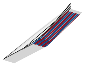
Figure 1. Schematic of the flow structure over a compression corner. Red solid line: boundary of the computational domain. Here LES, leading-edge shock; SS, separation shock; RS, reattachment shock; SL, slip line; EW, expansion wave.
Figure 1 shows the schematic of the basic flow structure over a compression corner configuration. A weak leading-edge shock (LES) is generated because of viscous interaction. A separation region is formed near the corner due to the adverse pressure gradient caused by the flow deflection. The separation region further induces a separation shock (SS) and a reattachment shock (RS), which interact with each other and result in a slip line (SL) and an expansion wave (EW). Essentially, the flow structure resembles Edney's type VI shock interaction (Edney Reference Edney1968).
3.2. Spatial and temporal discretization
The numerical simulations in this study are performed using an in-house multi-block parallel finite-volume solver called PHAROS (Hao, Wang & Lee Reference Hao, Wang and Lee2016; Hao & Wen Reference Hao and Wen2020). The modified Steger–Warming scheme (MacCormack Reference Maccormack2014) extended to a higher order by the monotone upstream-centred schemes for conservation law reconstruction (van Leer Reference van Leer1979) is used to calculate the inviscid fluxes, whereas a second-order central difference is used to compute the viscous fluxes. An implicit line relaxation method (Wright, Candler & Bose Reference Wright, Candler and Bose1998) is employed for time integration.
Computational meshes are constructed with three levels of grid refinement including 800 × 200 (coarse), 1200 × 400 (medium) and 1600 × 600 (fine) in the streamwise and wall-normal directions. The normal spacing at the surfaces is set to 1 × 10⁻⁷ m to ensure that the grid Reynolds number has an order of magnitude of one. The boundary conditions are specified as follows: the free-stream conditions are applied to the upper and left boundaries. A simple extrapolation outflow condition is used at the exit boundary. The wall is assumed to be isothermal and no slip. All the simulations in the present study are run with a constant Courant–Friedrichs–Lewy number of 103. Numerical convergence is achieved under the criteria that the Euclidean norm of the density residual is reduced by ten orders of magnitude, and the length of the separation region remains unchanged.
Figure 2 compares the surface distributions of skin friction coefficient Cf and surface pressure coefficient Cp obtained using three different meshes for α = 15 ° and Tw/T 0 = 0.86. In fact, this flow condition has the largest separation region among the cases considered in this study. The Cf and Cp are defined by
 \begin{equation}{C_f} = \frac{{{\tau _w}}}{{0.5{\rho _\infty }u_\infty ^2}},\quad {C_p} = \frac{{{p_w}}}{{0.5{\rho _\infty }u_\infty ^2}},\end{equation}
where τw and pw are the wall shear stress and pressure, respectively. Flow separation and reattachment occur at the most upstream and downstream locations where the curve of Cf crosses zero. Herein, the length of the separation region is defined as the distance between the separation and reattachment points in the x direction. It is seen that the length of the separation region is underestimated by using the coarse grid. As the grid is refined, the separation region is enlarged and approaches a certain value. The pressure and skin friction distributions obtained on the medium and fine grids are almost overlapped, which indicates that the medium grid (1200 × 400) is adequate to guarantee grid independence.
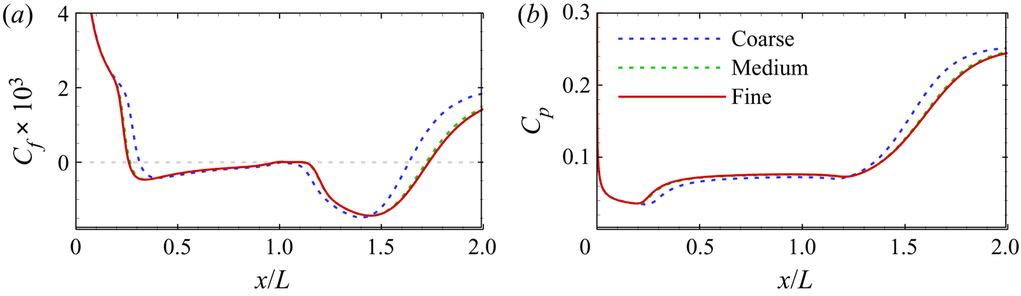
Figure 2. Distributions of (a) skin friction coefficient and (b) surface pressure coefficient obtained using three different meshes for α = 15 ° and Tw/T 0 = 0.86.
3.3. Global stability analysis
The vector of conservative variables U is decomposed into a 2-D steady solution  $\boldsymbol{U}_{2\textrm{-}{\rm D}}$ and a 3-D small-amplitude perturbation U′ as
 \begin{equation}\boldsymbol{U}(x,y,z,t) = {\boldsymbol{U}_{2\text{-D}}}(x,y) + {\boldsymbol{U}^{\prime}}(x,y,z,t).\end{equation}
The linearized Navier–Stokes equations (LNS) that describe the behaviour of U′ can be obtained by substituting (3.2) into the governing equations (2.1) and neglecting higher-order terms. The LNS are then discretized using a second-order finite-volume method. The modified Steger–Warming scheme is used to evaluate the inviscid Jacobians on cell faces near discontinuities, which are detected by an improved Ducros shock sensor (Hendrickson, Kartha & Candler Reference Hendrickson, Kartha and Candler2018). To reduce numerical dissipation, a central scheme is activated in smooth regions. The viscous Jacobians are computed using the second-order central difference. Details of the inviscid and viscous Jacobians were given by Sidharth et al. (Reference Sidharth, Dwivedi, Candler and Nichols2018).
The initial value problem is transformed to an eigenvalue problem by expressing the vector of perturbed conservative variables U′ in the following modal form:
 \begin{equation}{\boldsymbol{U}^{\prime}}(x,y,z,t) = \hat{\boldsymbol{U}}(x,y)\ \textrm{exp}\left( { - \textrm{i}\omega t + \textrm{i}\frac{{2{\rm \pi} }}{\lambda }z} \right),\end{equation}
where  $\hat{\boldsymbol{U}}$ is the 2-D eigenfunction, ω is the eigenvalue and λ is the spanwise wavelength. In fact, the current GSA considers the temporal stability of a spanwise periodic perturbation superimposed on a 2-D steady solution, i.e. a bi-global analysis. The eigenvalue problem is solved using the implicit restarted Arnoldi method implemented in ARPACK (Reference Sorensen, Lehoucq, Yang and MaschhoffSorensen et al. 1996) for a given λ. A shift-invert approach is employed to efficiently explore the eigenvalue spectra. The obtained eigenvalues are complex numbers with the real and imaginary parts ωr and ωi representing the angular frequency and growth rate, respectively. Note that a positive ωi indicates an unstable mode.
The GSA with the shift-invert approach can be computationally expensive, especially in memory usage, because a lower--upper decomposition of the global matrix is performed in the inversion step. To reduce the computational burden, the 2-D base flows are interpolated on a coarser grid (600 × 300) for stability analysis. Grid independence was verified by using a finer grid (800 × 400). On the wall, the velocity and temperature perturbations and the wall-normal gradient of pressure perturbation are set to zero. A sponge layer is implemented near the far field and outflow boundaries of the computational domain to ensure no reflection of perturbations (Mani Reference Mani2012).
4. Results
4.1. General flow features
Figure 3 shows the 2-D steady distributions of skin friction coefficient for different ramp angles and wall temperature ratios. Also shown in the figure are the enlarged views near the corner. The separation and reattachment points are indicated by open circles. For a fixed Tw/T 0, the separation and reattachment points move upstream and downstream, respectively, as the ramp angle is increased. Inside the separation region, there are two local minima of Cf. As reported by Smith & Khorrami (Reference Smith and Khorrami1991), Korolev, Gajjar & Ruban (Reference Korolev, Gajjar and Ruban2002) and Gai & Khraibut (Reference Gai and Khraibut2019), the magnitude of the second minimum increases with α. There is a local skin friction peak between the two minima near the corner, which also increases with α. Beyond a certain ramp angle, the local peak becomes positive, indicating the emergence of secondary separation. For Tw/T 0 = 0.18, a secondary bubble occurs when α is around 13 °–14 °, whereas the critical value is approximately 14 °–15 ° for Tw/T 0 = 0.54 and 0.86. In general, the occurrence of the secondary separation is postponed to a larger ramp angle as the wall temperature is increased, which is consistent with the observation of Shvedchenko (Reference Shvedchenko2009). Downstream of the reattachment point, the skin friction rises to its peak value and then decreases gradually. Note that there is a local increase in Cf further downstream for Tw/T 0 = 0.18, which is caused by the impingement of EW induced by the shock interaction between SS and RS (see figure 1).
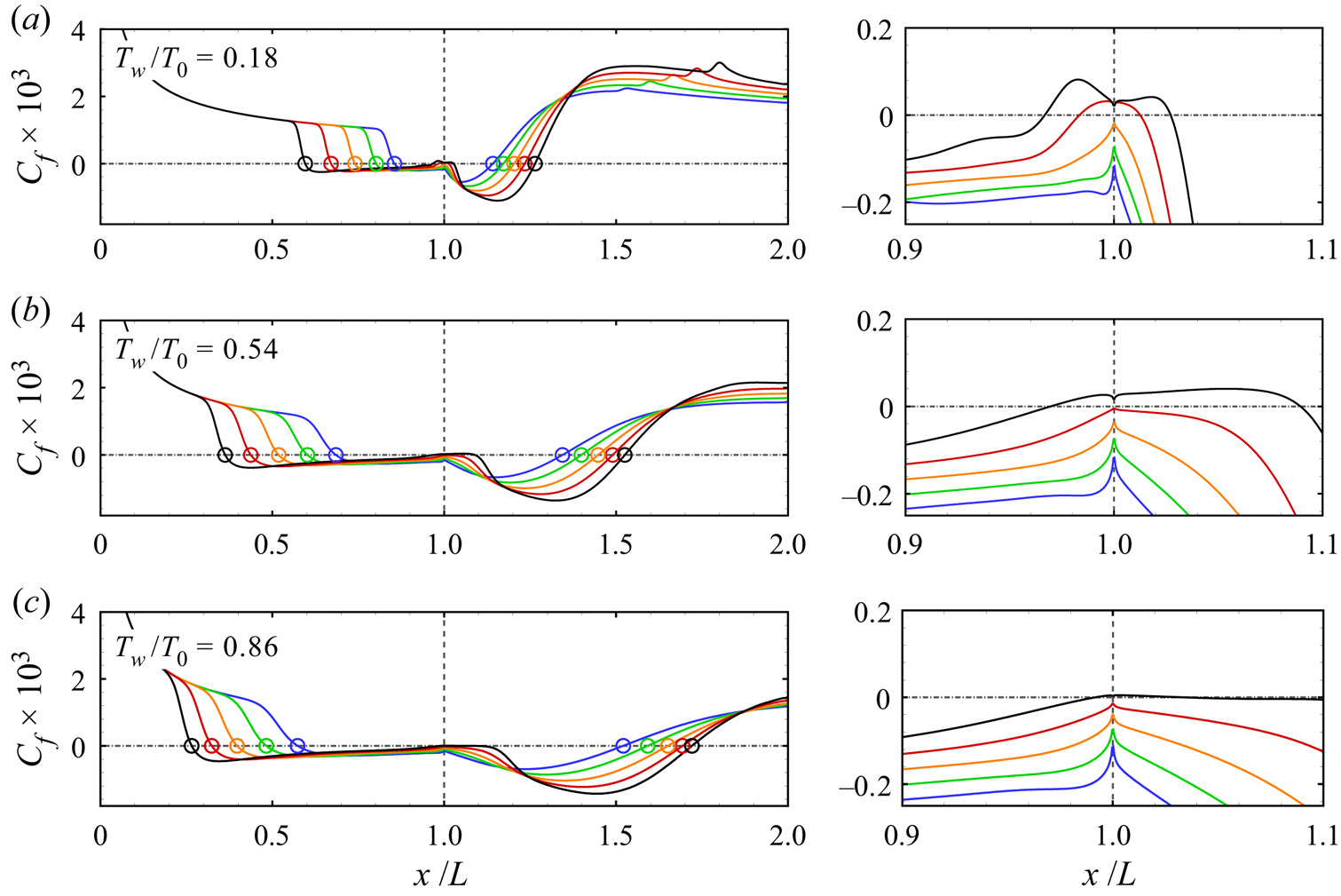
Figure 3. Distributions of skin friction coefficient for different ramp angles with the enlarged views near the corner: (a) Tw/T 0 = 0.18; (b) Tw/T 0 = 0.54; (c) Tw/T 0 = 0.86. Open circles: separation and reattachment points. Blue, α = 11 °; green, α = 12 °; orange, α = 13 °; red, α = 14 °; black, α = 15 °.
Figure 4 shows the 2-D steady distributions of surface pressure coefficient for different ramp angles and wall temperature ratios. The surface pressure begins to increase upstream of the separation point controlled by the free-interaction process (Chapman, Kuehn & Larson Reference Chapman, Kuehn and Larson1958). The rise is followed by a plateau region, the value of which increases with α and Tw/T 0. It is consistent with the free-interaction theory that the plateau pressure is inversely proportional to the Reynolds number based on the distance between the leading edge and separation point. The pressure rises again near the reattachment point and reaches its peak value mainly determined by the oblique shock theory. As the wall temperature is increased, the increase in Cp near reattachment becomes more gradual. For Tw/T 0 = 0.18, the drop in Cp downstream of the peak is also caused by the impingement of EW. For relatively large ramp angles, there is a small ‘dip’ in the surface pressure between the plateau and peak. Similar features have also been observed by Smith & Khorrami (Reference Smith and Khorrami1991), Korolev et al. (Reference Korolev, Gajjar and Ruban2002) and Gai & Khraibut (Reference Gai and Khraibut2019). As will be seen later, the ‘dip’ is indicative of a local region with pressure gradient near the corner, which becomes stronger as α is increased such that the reverse flow boundary layer cannot resist it and gives rise to secondary separation.
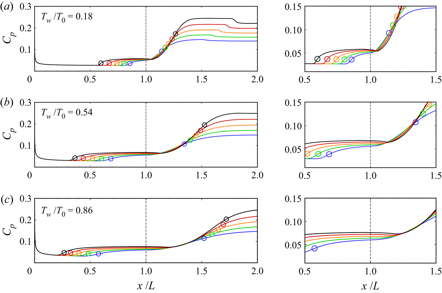
Figure 4. Distributions of surface pressure coefficient for different ramp angles with the enlarged views near the corner: (a) Tw/T 0 = 0.18; (b) Tw/T 0 = 0.54; (c) Tw/T 0 = 0.86. Open circles: separation and reattachment points. Blue, α = 11 °; green, α = 12 °; orange, α = 13 °; red, α = 14 °; black, α = 15 °.
Contours of 2-D density gradient magnitude and pressure (near the compression corner) non-dimensionalized by  ${\rho _\infty }u_\infty ^2$ are plotted with the streamlines inside the separation region superimposed in figure 5 for Tw/T 0 = 0.18. Only the flow fields with the ramp angles of 13 °, 14 °, and 15 ° are presented to focus on the emergence of secondary separation. There is no secondary separation at α = 13 °, and the core of the primary vortex is located above the ramp surface downstream of the corner. At α = 14 °, a secondary vortex occurs beneath the primary bubble near the corner. The secondary bubble grows in both horizontal and vertical extents as α is increased to 15 °, while the primary bubble fragments into two vortices. As demonstrated by Shvedchenko (Reference Shvedchenko2009), Egorov et al. (Reference Egorov, Neiland and Shvedchenko2011) and Gai & Khraibut (Reference Gai and Khraibut2019), further increasing the ramp angle leads to fragmentation into multiple vortices and eventually unsteadiness for 2-D laminar simulations.
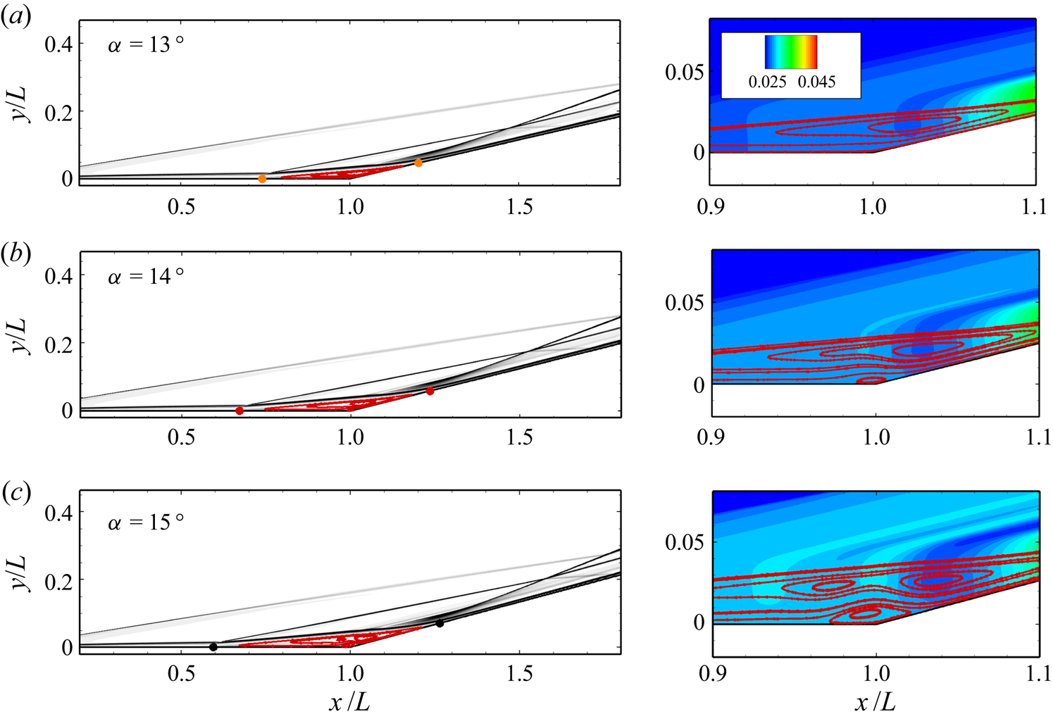
Figure 5. Contours of density gradient magnitude (left column) and non-dimensional pressure (right column) with streamlines superimposed for Tw/T 0 = 0.18: (a) α = 13 °; (b) α = 14 °; (c) α = 15 °. Closed circles: separation and reattachment points.
At α = 13 °, a low-pressure region can be seen in the vortex core, which balances the centrifugal force of a fluid element rotating about the core (Jeong & Hussain Reference Jeong and Hussain1995). It can be speculated that the ‘dip’ of surface pressure is the footprint of this low-pressure region on the ramp surface. This low-pressure region also stretches out of the separation region in the form of a weak expansion wave. As α is increased, the low pressure in the primary-vortex core only changes slightly; however, the pressure in the upstream half of the separation region is obviously elevated in accordance with the variation of the plateau pressure (see figure 4). Such a behaviour poses a local streamwise adverse pressure gradient to the reverse flow boundary layer developing from the reattachment point. With the emergence of primary-vortex fragmentation and secondary separation, multiple waves emanate from the separation region.
The corresponding non-dimensionalized pressure gradients in the x and y directions are compared in figure 6 for Tw/T 0 = 0.18 and different ramp angles. The separation and reattachment points and the dividing streamline are also plotted to mark the extent of the separation region. As α in increased, the streamwise pressure gradient (px) inside the separation bubble near the corner becomes progressively intensified. Beyond a certain value, the reverse flow boundary layer separates to form a secondary bubble. Meanwhile, the emergence of secondary separation deforms the primary bubble, resulting in a transverse pressure gradient (py). Similar observations were made by Khraibut et al. (Reference Khraibut, Gai, Brown and Neely2017) for a hypersonic leading-edge separation.
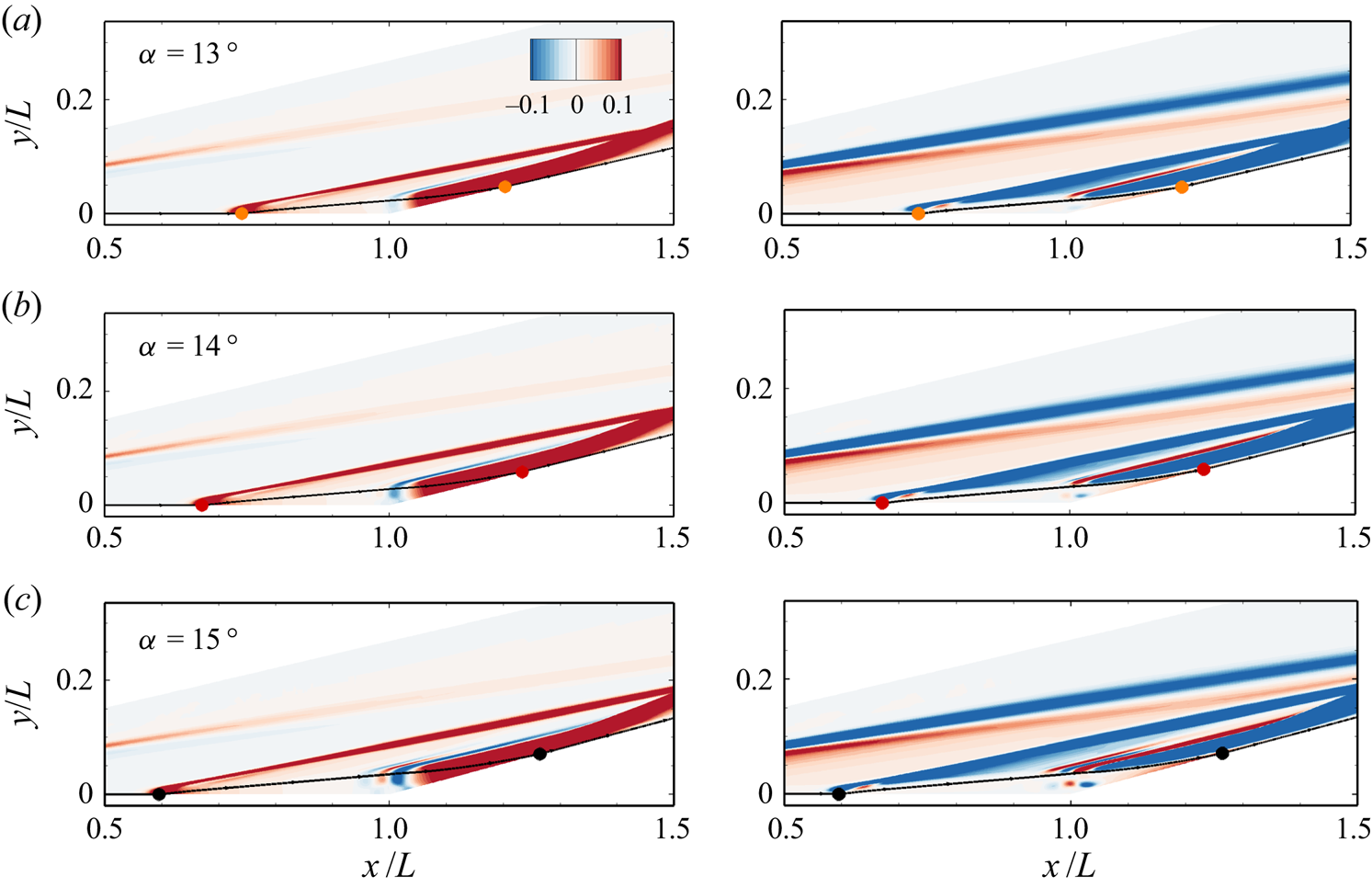
Figure 6. Contours of non-dimensional streamwise (left column) and transverse (right column) pressure gradients with dividing streamlines superimposed for Tw/T 0 = 0.18: (a) α = 13 °; (b) α = 14 °; (c) α = 15 °. Closed circles: separation and reattachment points.
Figure 7 shows the contours of density gradient magnitude and non-dimensionalized streamwise pressure gradient for the hot-wall cases at α = 15 °. For Tw/T 0 = 0.54, the separation region is significantly enlarged compared with the cold-wall condition. However, the occurrence of the secondary bubble is postponed until α = 15 ° and no fragmentation of the primary bubble is observed. Meanwhile, the core of the secondary bubble is shifted downstream of the corner. For the adiabatic-wall condition (Tw/T 0 = 0.86), only an incipient secondary separation can be seen. Clearly, the strength of the streamwise pressure gradient in the separation region is weakened by elevating the wall temperature, which is responsible for the delay of secondary separation.
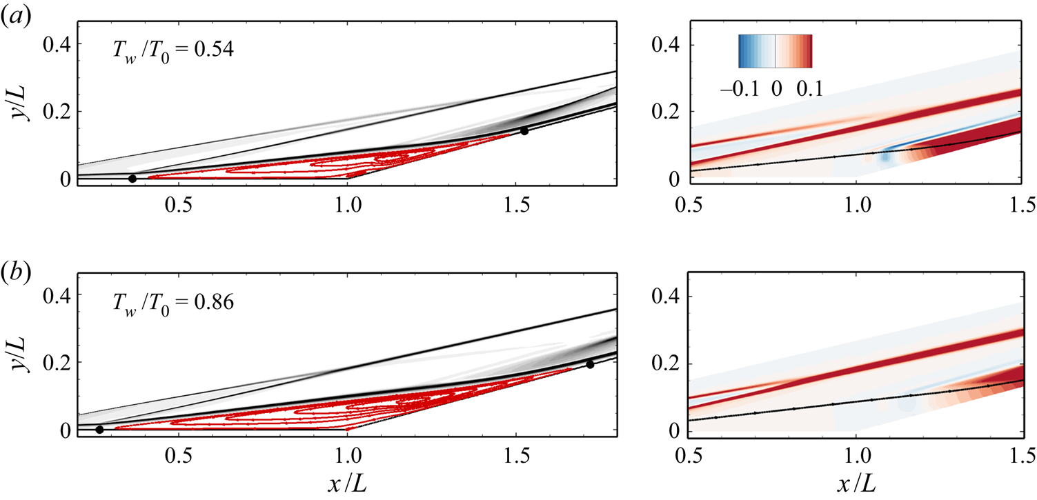
Figure 7. Contours of density gradient magnitude (left column) and non-dimensional streamwise pressure gradient (right column) with streamlines superimposed at α = 15 °: (a) Tw/T 0 = 0.54 and (b) Tw/T 0 = 0.86. Closed circles: separation and reattachment points.
To closely examine the reverse flow boundary layer, wall-normal distributions of flow quantities are extracted through the core of the primary vortex located downstream of the corner for different wall temperatures at α = 15 °. Figure 8 plots the profiles of streamwise velocity (u) and its streamwise gradient (ux) as a function of normal distance from the wall (yn). The locations of the vortex core are marked by closed circles. There is no clear definition of reverse flow boundary layer. Herein, it is defined as the reverse flow region beneath the vortex core as seen in figure 8(a). A maximum reverse flow velocity can be observed between the vortex core and wall, which increases with increasing wall temperature. Above the vortex core, the rapid change in the streamwise velocity corresponds to the shear layer induced by the separation region. In figure 8(b), there are two local minima separated by the vortex core, representing strong deceleration in the shear layer and reverse flow boundary layer, respectively. The magnitude of the minimum in the reverse flow boundary layer is reduced with increasing wall temperature, which may result from the weakened streamwise pressure gradient.
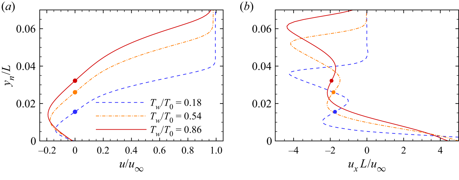
Figure 8. Distributions of (a) streamwise velocity and (b) streamwise gradient of streamwise velocity extracted along the wall-normal direction through the core of the primary vortex as a function of distance from the wall for different wall temperatures at α = 15 °. Closed circles: vortex core.
4.2. Occurrence of global instability
To determine the global stability of the hypersonic compression corner flows with respect to periodic spanwise perturbations, GSA is performed with the 2-D steady solutions obtained in § 4.1 as the base flows over a wide range of spanwise wavelengths.
Figure 9 presents the growth rates of the least stable mode as a function of spanwise wavelength for different ramp angles and wall temperature ratios. Open symbols represent stationary modes with ωr = 0, whereas closed symbols denote oscillating modes with ωr ≠ 0. For Tw/T 0 = 0.18, the flow system is globally stable to 3-D perturbations at α = 12 °, although not shown here. At α = 13 °, the separated flow becomes unstable with the largest growth rate occurring at λ/L = 0.168. The captured least stable mode is largely stationary, which is oscillating only for short spanwise wavelengths. As α is further increased to 14 °, the stationary unstable mode is shifted to a larger wavelength. Meanwhile, the growth rate of the oscillating mode increases significantly and dominates over its stationary counterpart. Essentially, they belong to the same branch of eigenvalues. As the spanwise wavelength is decreased, the pure imaginary eigenvalue corresponding to the stationary mode leaves the imaginary axis to form two conjugate eigenvalues. At α = 15 °, the conjugate eigenvalues merge again, resulting in a strongly unstable stationary mode at λ/L = 0.066. For Tw/T 0 = 0.54 and 0.86, the flows are marginally stable when α = 13 ° and become unstable at α = 14 °. The behaviour of the most unstable mode is similar to that for the cold-wall condition, i.e. the stationary mode is shifted to a longer wavelength as α is increased and an unstable mode occurs at a shorter wavelength and becomes dominant.
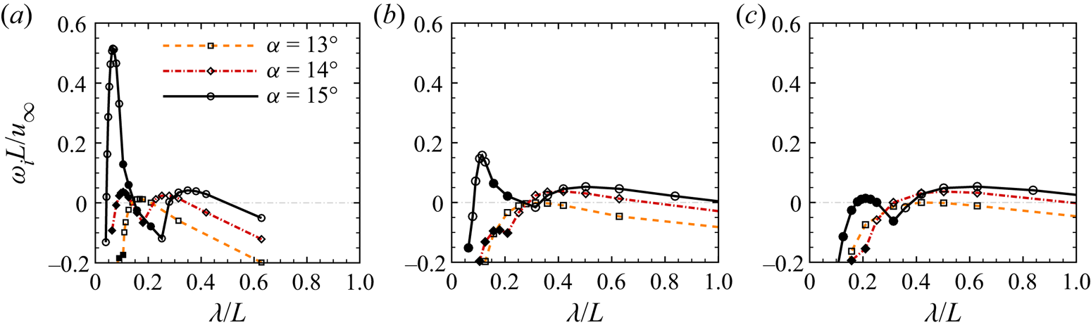
Figure 9. Growth rates of the most unstable mode as a function of spanwise wavelength for different ramp angles: (a) Tw/T 0 = 0.18; (b) Tw/T 0 = 0.54; (c) Tw/T 0 = 0.86. Open symbols: stationary. Closed symbols: oscillating modes.
For the cold-wall condition, the flow system is unstable when 12 ° < α < 13 °. For the hot-wall conditions, the critical ramp angles are 13 °–14 °. The GSA reveals that the global instability of the hypersonic compression corner flow is closely linked with the emergence of secondary separation. Elevating the wall temperature stabilizes the flow system, although the length of the separation region is considerably enlarged.
Figure 10 shows the contours of the real part of the spanwise velocity perturbation ŵ/u ∞ corresponding to the short-wavelength unstable modes at their respective most unstable wavelengths (i.e. λ/L = 0.066, 0.114, and 0.209) for different wall temperatures at α = 15 °. Note that the short-wavelength mode dominates over the long-wavelength mode as α is increased to a certain value. The corresponding eigenvalue spectra at these conditions are also plotted. Grid independence was verified by comparing the eigenvalues obtained on the coarse (600 × 300) and fine (800 × 400) grids for Tw/T 0 = 0.18. The spanwise velocity perturbations are mainly confined to the separation region for different wall temperatures. In the downstream portion of the separation bubble, the spanwise velocity perturbations are highly distorted in a pattern of alternating positive and negative components. For Tw/T 0 = 0.18, the eigenfunction structurally resembles the GSA result of Sidharth et al. (Reference Sidharth, Dwivedi, Candler and Nichols2017) for a heated compression corner. As seen from the spectrum, two oscillating unstable modes are captured with the non-dimensionalized frequencies fL/u ∞ of 0.225 and 0.578, respectively, where f = ωr/2 ${\rm \pi}$. The frequencies agree well with the DNS results of Cao et al. (Reference Cao, Hao, Klioutchnikov, Olivier and Wen2021). As the wall temperature is increased, the growth rate of the most unstable mode decreases, which becomes an oscillating mode for the adiabatic-wall condition (Tw/T 0 = 0.86). Meanwhile, the two oscillating unstable modes are stabilized and eventually merge with the continuous modes.

Figure 10. Contours of real part of spanwise velocity perturbation (left column) and eigenvalue spectra (right column) for α = 15 °: (a) Tw/T 0 = 0.18 at λ/L = 0.066; (b) Tw/T 0 = 0.54 at λ/L = 0.114; (c) Tw/T 0 = 0.86 at λ/L = 0.209. Closed circles: separation and reattachment points. Open circles in the eigenvalue spectra: eigenvalues obtained on a coarse grid (600 × 300). Open squares in the eigenvalue spectra: eigenvalues obtained on a fine grid (800 × 400).
Figure 11 shows the contours of the real part of  $\hat{w}/{u_\infty }$ and the eigenvalue spectra corresponding to the long-wavelength unstable modes at their respective most unstable wavelengths (i.e. λ/L = 0.349, 0.503 and 0.628) for different wall temperatures at α = 15 °. The spanwise velocity perturbation is mostly confined to the separation region with an opposite sign in the upstream and downstream halves, which is similar to the GSA result of Sidharth et al. (Reference Sidharth, Dwivedi, Candler and Nichols2018) for a double-wedge configuration. In contrary to the short-wavelength scenario, only one stationary unstable mode can be identified.

Figure 11. Contours of real part of spanwise velocity perturbation (left column) and eigenvalue spectra (right column) for α = 15 °: (a) Tw/T 0 = 0.18 at λ/L = 0.349; (b) Tw/T 0 = 0.54 at λ/L = 0.503; (c) Tw/T 0 = 0.86 at λ/L = 0.628. Closed circles: separation and reattachment points.
To further understand the physical mechanisms that drive the global instability of the separation bubble, an energy budget analysis is performed for the short-wavelength unstable modes corresponding to different wall temperatures as shown in figure 10 at α = 15 °. According to previous GSA studies on laminar flow separation (Theofilis et al. Reference Theofilis, Hein and Dallmann2000; Sidharth et al. Reference Sidharth, Dwivedi, Candler and Nichols2018; Cao et al. Reference Cao, Hao, Klioutchnikov, Olivier and Wen2021), the global instability induces three-dimensionality in the separation bubble and alters its topological structure, which indicates that the disturbance field is mainly characterized by velocity perturbations. Hence, only the kinetic disturbance energy is considered here, which contributes more than 70 % of the total disturbance energy quantified by the Chu energy norm (Chu Reference Chu1965).
The linearized governing equation of velocity perturbations is given by
 \begin{equation}\frac{{\partial {{u^{\prime}}_i}}}{{\partial t}} + {\bar{u}_j}\frac{{\partial {{u^{\prime}}_i}}}{{\partial {x_j}}} ={-} \frac{{{{(\rho {u_j})}^\prime }}}{{\bar{\rho }}}\frac{{\partial {{\bar{u}}_i}}}{{\partial {x_j}}} - \frac{1}{{\bar{\rho }}}\frac{{\partial p^{\prime}}}{{\partial {x_i}}} - \frac{1}{{\bar{\rho }}}\frac{{\partial {{\tau ^{\prime}}_{ij}}}}{{\partial {x_j}}},\end{equation}
where indices i = 1, 2 and 3 represent the x, y and z directions, respectively. The specific kinetic disturbance energy is defined by
 \begin{equation}{e^{\prime}_k} = \frac{1}{2}u^{\prime}{u^{\prime}_i}^{\dagger} ,\end{equation}
where † is used to denote the complex conjugate. The governing equation of  ${e^{\prime}_k}$ can be obtained by taking the dot product of (4.1) and ${u^{\prime}_i}^{\dagger}$ as
 \begin{equation}\frac{{\partial {{e^{\prime}}_k}}}{{\partial t}} = Re \left[ { - {{\bar{u}}_j}{{u^{\prime}}_i}^{\dagger} \frac{{\partial {{u^{\prime}}_i}}}{{\partial {x_j}}} - {{u^{\prime}}_i}^{\dagger} \frac{{{{(\rho {u_j})}^\prime }}}{{\bar{\rho }}}\frac{{\partial {{\bar{u}}_i}}}{{\partial {x_j}}} - \frac{{{{u^{\prime}}_i}^{\dagger} }}{{\bar{\rho }}}\frac{{\partial p^{\prime}}}{{\partial {x_i}}} - \frac{{{{u^{\prime}}_i}^{\dagger} }}{{\bar{\rho }}}\frac{{\partial {{\tau^{\prime}}_{ij}}}}{{\partial {x_j}}}} \right],\end{equation}
where Re denotes the real part of a complex number. Note that the perturbed variables can be written in a modal form as given by (3.3). One can readily obtain the following expression:
 \begin{equation}{e^{\prime}_k} = {\hat{e}_k}\ \textrm{exp}(2{\omega _i}t),\end{equation}
where  ${\hat{e}_k}$ is the eigenfunction of the kinetic disturbance energy. Substituting (4.4) into (4.3) leads to
 \begin{equation}2{\omega _i}{\hat{e}_k} = Re \left[ {\underbrace{{ - {{\bar{u}}_j}{{\hat{u}}_i}^{\dagger} \frac{{\partial {{\hat{u}}_i}}}{{\partial {x_j}}}}}_{{Convection}}\underbrace{{ - {{\hat{u}}_i}^{\dagger} \frac{{\widehat {\rho {u_j}}}}{{\bar{\rho }}}\frac{{\partial {{\bar{u}}_i}}}{{\partial {x_j}}}}}_{{Production}}\underbrace{{ - \frac{{{{\hat{u}}_i}^{\dagger} }}{{\bar{\rho }}}\frac{{\partial \hat{p}}}{{\partial {x_i}}}}}_{{Transfer}}\underbrace{{ - \frac{{{{\hat{u}}_i}^{\dagger} }}{{\bar{\rho }}}\frac{{\partial {{\hat{\tau }}_{ij}}}}{{\partial {x_j}}}}}_{{Viscous}}} \right],\end{equation}
where the convection term represents the advection of  ${\hat{e}_k}$ by the mean velocity, the production term is the work done by the Reynolds stress on the mean velocity gradient, the transfer term is the energy transport due to velocity and pressure fluctuations and the viscous term accounts for the molecular dissipation effects.
Following Mittal (Reference Mittal2010), we integrate (4.5) over the entire computational domain to obtain the following equation:
 \begin{equation}{\omega _i} = {\omega _{i,convection}} + {\omega _{i,production}} + {\omega _{i,transfer}} + {\omega _{i,viscous}},\end{equation}
where ωi ,convection, ωi ,production, ωi ,transfer and ωi ,viscous are the contributions to the total growth rate due to different mechanisms. Variations of these growth rate components for the short-wavelength unstable modes are plotted in figure 12 as a function of wall temperature ratio. The total growth rate is mainly contributed by the production term, whereas the convection and transfer terms are negligible. As the wall temperature is increased, the production term is significantly reduced.

Figure 12. Variation of growth rate components for the short-wavelength unstable modes at λ/L = 0.066, 0.114 and 0.209 as a function of wall temperature ratio for α = 15 °.
Figure 13 shows the spatial distributions of the production term for the short-wavelength unstable modes corresponding to different wall temperatures. The production term is localized near the primary-vortex core, which confirms that the instability arises from the separation region. Distributions of the production term are also plotted in this figure in the wall-normal direction through the vortex core. Close examination of the production term reveals that the major contribution comes from the streamwise gradient of the streamwise velocity (ux), which is consistent with the finding of Sidharth et al. (Reference Sidharth, Dwivedi, Candler and Nichols2018). Comparing with figure 8(b), one can see that it is the deceleration of the reverse flow boundary layer instead of the shear layer that leads to the peak production of the kinetic disturbance energy. Increasing the wall temperature alleviates this deceleration due to the weakened streamwise pressure gradient (see figures 4 and 7), which explains the suppression of global instability. Similar behaviours were observed near the critical ramp angle of global instability. Deceleration of the streamwise velocity in the reverse flow boundary layer becomes stronger with increasing ramp angle, which results in a production term prevailing over the viscous term.

Figure 13. Contours of production term in the kinetic disturbance energy equation with streamlines superimposed (left column) and its distribution extracted along the wall-normal direction through the core of the primary vortex as a function of distance from the wall (right column) for α = 15 °: (a) Tw/T 0 = 0.18 at λ/L = 0.066; (b) Tw/T 0 = 0.54 at λ/L = 0.114; (c) Tw/T 0 = 0.86 at λ/L = 0.209. Closed circles: vortex core.
4.3. Criterion in terms of triple-deck scaling
This study reveals that the occurrence of both secondary separation and global instability are governed by the characteristics of the reverse flow boundary layer. To describe the behaviour of flow separation, an asymptotic theory known as the triple-deck theory was established by Neiland (Reference Neiland1969) and Stewartson & Williams (Reference Stewartson and Williams1969) using the method of matched asymptotic expansions. They divided the boundary layer upstream of separation into three decks, including a viscous lower deck, an inviscid and rotational middle deck and an inviscid and irrotational upper deck. By introducing a specific set of scaled variables, the governing equations in the lower deck were reduced to the incompressible boundary-layer equations, which can be efficiently solved. Most importantly, the characteristic scaling defined by the triple-deck theory provides an effective approach to correlate and interpret numerical and experimental data in terms of a scaled ramp angle α*. According to Stewartson & Williams (Reference Stewartson and Williams1969), α* is defined by
 \begin{equation}{\alpha ^ \ast } = \frac{{\alpha {Re}_L^{1/4}}}{{{C^{1/4}}{{0.332}^{1/2}}{{(M_\infty ^2 - 1)}^{1/4}}}},\quad C = \frac{{{\mu _w}{T_\infty }}}{{{\mu _\infty }{T_w}}},\end{equation}
where C is the Chapman–Rubesin parameter.
The triple-deck theory was initially applied to incipient or small-scale separation. As α* is increased, a pressure plateau was formed by solving the triple-deck equations (Rizzetta, Burggraf & Jenson Reference Rizzetta, Burggraf and Jenson1978). Smith & Khorrami (Reference Smith and Khorrami1991) suggested that there was a critical value of α* beyond which a singularity developed near reattachment in the triple-deck solution. However, Korolev et al. (Reference Korolev, Gajjar and Ruban2002) found that the computational domain used by Smith & Khorrami (Reference Smith and Khorrami1991) was insufficient to resolve the flow problem. Secondary separation was observed near the corner inside the separation region for a large α*. They also confirmed that the scaled length of the separation region was linearly proportional to α*3/2 for a large separation region, as suggested by Burggraf (Reference Burggraf1975). It was indicated that the triple-deck theory can be extended to moderate- to large-scale separation problems.
In the present study, the secondary separation occurs when α* is 3.73–4.92, which is consistent with the findings of Smith & Khorrami (Reference Smith and Khorrami1991), Korolev et al. (Reference Korolev, Gajjar and Ruban2002), Shvedchenko (Reference Shvedchenko2009) and Gai & Khraibut (Reference Gai and Khraibut2019). Note that different definitions of scaled ramp angle were used in these studies. The lower and upper boundaries correspond to the cold- and adiabatic-wall conditions, respectively. A similar trend was observed by Egorov et al. (Reference Egorov, Neiland and Shvedchenko2011). Then, a criterion can be established in terms of α* to predict the stability boundary, i.e. 3.44 < α* < 4.59. Again, a higher wall temperature results in a larger critical ramp angle.
Figure 14 presents the variation of the critical scaled ramp angle as a function of wall temperature ratio. The error bars represent an uncertainty of 1 °, which is the minimum increment in ramp angle considered in this study. Additional simulations and GSA were performed for Tw/T 0 = 0.18 with ReL = 2.1 × 10⁵ and 8.4 × 10⁵, respectively. For the lower Reynolds number, the flow becomes globally unstable when α is 15 °–16 °, whereas secondary separation occurs when α is 16 °–17 °. For the larger Reynolds number, the critical ramp angles for global instability and secondary separation are 10 °–11 ° and 11 °–12 °, respectively. As expected, the resulting scaled ramp angles are almost overlapped, which indicates that the effect of the Reynolds number is well accounted for.

Figure 14. The critical scaled ramp angle for global instability as a function of wall temperature ratio. Open symbols: globally stable. Closed symbols: globally unstable.
Also shown in the figure are existing theoretical, numerical and experimental data collected from the literature for hypersonic compression corner and double-wedge flows with the free-stream Mach numbers ranging from 5 to 11.63 and the unit Reynolds numbers from 4.0 × 10⁵ m−1 to 13.6 × 10⁶ m−1. The detailed flow conditions are provided in table 1. For the double-wedge flows, α represents the angle between the first and second wedges, and the scaled ramp angle is evaluated using the flow properties behind the oblique shock induced by the first wedge. For the theoretical studies, it is straightforward to determine whether a flow system is globally unstable based on the GSA predictions. For example, the Mach 5 double-wedge flow considered by Sidharth et al. (Reference Sidharth, Dwivedi, Candler and Nichols2018) was found to be marginally stable when the turn angle is 7.8 ° and unstable for 10 °. For the computational fluid dynamics simulations, a flow is considered to be globally unstable only if 3-D streamwise streaks can be formed with no external disturbance. As for the experimental data, an observation of streamwise streaks is a necessary but not sufficient condition for global instability, as demonstrated by Dwivedi et al. (Reference Dwivedi, Sidharth, Nichols, Candler and Jovanović2019). Here, only those experimental data that have been confirmed by GSA are included. The proposed criterion clearly demarcates the stability boundary. Extension to shock impingement on a flat plate and axisymmetric flows will be the focus of a future study.
Table 1. Flow conditions of the theoretical, numerical and experimental data collected in figure 14.

Furthermore, it is important to note that no experimental evidence of secondary separation has been found. The speculation that the secondary separation leads to three-dimensionality and unsteadiness remains to be experimentally verified.
5. Conclusions
Hypersonic compression corner flows are numerically simulated to investigate the onset of global instability with varying ramp angles and wall temperatures. Secondary separation occurs when the ramp angle is beyond a certain value, which increases slightly with the wall temperature ratio. It is demonstrated that the secondary bubble arises from the flow separation of the reverse flow boundary layer under the action of an adverse pressure gradient, which is alleviated by increasing the wall temperature.
The GSA reveals that the flow becomes globally unstable as the ramp angle is increased. The unstable mode is shifted to a longer wavelength with increasing wall temperature. Beyond the critical ramp angle, a short-wavelength unstable mode is significantly destabilized and becomes dominant. Most importantly, it is found that the global instability occurs immediately prior to the emergence of the secondary separation. A kinetic energy budget analysis reveals that the global instability is driven by the streamwise flow deceleration in the reverse flow boundary layer, which is weakened by increasing the wall temperature.
The numerical simulations and GSA illustrate that the secondary separation and global instability are closely linked with each other mainly determined by the characteristics of the reverse flow boundary layer. The numerical results are then interpreted using the triple-deck theory. A criterion is proposed in terms of a scaled ramp angle to predict the stability boundary for hypersonic compression corner and double-wedge flows, which agrees well with existing theoretical, numerical, and experimental studies. For flow conditions far beyond the stability boundary, strong three-dimensionality (e.g. streamwise streaks downstream of reattachment) and unsteadiness in the flow fields are expected.
Funding
This work is supported by the Hong Kong Research Grants Council (no. 15206519).
Declaration of interests
The authors report no conflict of interest.


 Open access