


Introduction
Cold rolling is a sheet metal forming process used to strengthen material properties through plastic deformation of the microstructure. This procedure produces parts with good dimensional accuracy and clean surface finishes. Typically, cold rolling is limited to compression ratios up to 50%. Thus, to accumulate high plastic strain in cold rolling, multiple passes are required to compress the thickness of the workpiece rather than performing it in one single, large compression stage. The plastic deformation and friction between the workpiece and rollers cause the workpiece temperatures to rise. This can lead to deterioration of the rolls or softening of the workpiece. Pietrzyk and Lenard (Reference Pietrzyk and Lenard1991) investigated the heating of aluminum strips during deformation in cold rolling. Their analytical model accurately predicted the final temperatures with an error of below 1.5°C compared with experimental results. Other authors have extended their work to develop thermo-mechanical models for measuring temperatures in rolling processes (Chang, Reference Chang1998; Luo, Reference Luo1998).
Numerical methods have been used to analyze parameters’ effects (Hossain et al., Reference Hossain, Rafiei, Lachemi, Behdinan and Anwar2016) and investigate phenomenon that would otherwise be difficult to build experiments for (Kostiv et al., Reference Kostiv, Behdinan and Hashemi2012). In the context of cold rolling, Khan et al. (Reference Khan, Jamal, Arshed, Arif and Zubair2004) created a coupled thermo-mechanical heat transfer model based on the finite volume method. The study proved the impact of roll speed and heat transfer on heat flow distribution in both the roll and workpiece. Yadav et al. (Reference Yadav, Singh and Dixit2014) established an efficient FEM method for estimating temperature distributions in roll and strip in the order of seconds, which could be applied to both cold and hot rolling. Simplified mathematical models for heat transfer analysis were developed and validated against experimental results.
FEM has also been used for evaluating other important phenomena in cold rolling. Hwu and Lenard (Reference Hwu and Lenard1988) developed a finite element solution for evaluating the effects of work-roll deformation and friction on resulting strain fields in flat rolling. Liu et al. (Reference Liu, Hartley, Sturgess and Rowe1985) developed an elastic-plastic FEM for cold rolling of copper strips to determine stress and deformation outside the nominal contact. More recently, Mehrabi et al. (Reference Mehrabi, Salimi and Ziaei-Rad2015) studied chattering vibration in cold rolling using an implicit FEM method. From validating their FEM with experimental results, they determined the effects of friction and reduction on chatter and provided new design considerations in future rolling processes. FEMs are powerful tools for conducting engineering analyses and obtaining data on experiments which would otherwise be expensive to conduct. However, solving nonlinear problems is time-consuming and predictions become more difficult to obtain with higher complexity models. Artificial neural networks are a viable solution to these computational demands, which have not been explored for cold rolling simulations involving temperature rise due to plastic deformation.
Data mining has become a rapidly growing field in recent years due to a rise in data generation volume. This has led to a growth in size and complexity in data processing which continues to be a growing problem when efficiency and computation speed is important. High-dimensional data exists where the number of data features is on the order of the number of samples or observations (Narisetty, Reference Narisetty2020). These datasets can be computationally expensive to generate mapping functions between input and output. Thus, reducing the number of features, or the input dimensionality, can greatly simplify the learning and accelerate the training phase of regression and classification models for identifying patterns between features and output. Dimensionality reduction has been used extensively as a feature extraction tool for surrogate models, such as artificial neural networks (ANNs) and finite element analysis (FEA) research. Kashid and Kumar (Reference Kashid and Kumar2012) reviewed the current state-of-the-art applications of ANNs to sheet metal work. They critically reviewed the use of ANNs for reducing computation time and on bending operations. Their conclusions discuss the drawbacks on backpropagation in ANNs such as long training times and large data requirements in several works. Shahani et al. (Reference Shahani, Setayeshi, Nodamaie, Asadi and Rezaie2009) used FEM with ANNs to predict influential parameters in a 2D aluminum hot rolling process. The study used an updated Lagrangian method formulation to solve a thermo-mechanical analysis and determine the effects of process parameters. ANNs have also been optimized for predicting springback in sheet metal forming (Liu et al., Reference Liu, Liu, Ruan, Liang and Qiu2007; Ruan et al., Reference Ruan, Feng and Liu2008; Spathopoulos and Stavroulakis, Reference Spathopoulos and Stavroulakis2020). For instance, Spathopoulos et al. (Spathopoulos and Stavroulakis, Reference Spathopoulos and Stavroulakis2020) used a Bayesian regularized backpropagation neural network for predicting springback in the S-Rail metal forming process. In cold rolling, ANNs have been explored for predicting new mechanical properties (Ghaisari et al., Reference Ghaisari, Jannesari and Vatani2012) such as yield and ultimate tensile strength, degree of void closure (Chen et al., Reference Chen, Chandrashekhara, Mahimkar, Lekakh and Richards2011), defect detection (Yazdchi and Mahyari, Reference Yazdchi and Mahyari2008), and rolling force (Lin, Reference Lin2002). However, dimensionality reduction has not been applied to ANNs for improving the computation time and training of these surrogate models in cold rolling.
In terms of combining dimensionality reduction with neural networks, several authors have investigated these integrated methods for reducing computational cost of designing reduced-order models. Higdon et al. (Reference Higdon, Gattiker, WIlliams and Rightley2008) applied PCA for non-probabilistic, dimensionality reduction in Gaussian processes for uncertainty quantification of material properties. PCA has also improved optimization of surrogate models in calibration (Kamali et al., Reference Kamali, Ponnambalam and Soulis2007), aerodynamics (Kapsoulis et al., Reference Kapsoulis, Tsiakas, Trompoukis and Giannakoglou2018; Tao et al., Reference Tao, Sun, Guo and Wang2020), and air pollution (Olvera et al., Reference Olvera, Garcia, Li, Yang, Amaya, Myers, Burchiel, Berwick and Pingitore N2012). Straus et al. (Straus and Skogestad, Reference Straus and Skogestad2017) developed extended surrogate model fitting methods by incorporating PLS regression for reducing the number of independent variables in an ammonia process case study. The nonlinear surrogate models were fitted to the PLS latent variables and improved the surrogate model fit by a factor of two. Finally, PCA's applicability is limited to linearly separable datasets and projections onto a linear subspace. Thus, kernel PCA (kPCA)-based surrogate models have been used to reduce complexity in high-dimensionality datasets such as water quality forecasting (Zhang et al., Reference Zhang, Fitch and Thorburn2020) and intrusion detection (Hongwei and Liang, Reference Hongwei and Liang2008). However, DR-NNs have yet to be explored in prediction for cold rolling and other sheet metal applications.
In this work, we investigated the use of dimensionality reduction methods such as principal component analysis (PCA), partial least squares (PLS), and kPCA with neural network surrogate models for reducing computation times and uncertainty in predicting the change in temperature due to plastic deformation in a two-stage cold rolling FEM simulation. The paper is organized in the following manner. Section “Dimensionality Reduction” begins with a mathematical summary of the explored dimensionality reduction methods and neural network used and describes the general structure of the DR-NNs. Next, Section “Test Case: Finite Element Model” describes the FEA two-stage cold rolling test case used to evaluate the performance of our DR-NNs against standard neural networks. Section “Results and Discussion” shows the prediction error and computation time results of the DR-NNs and neural network and discusses the results and usefulness of dimensionality reduction for neural networks, as well as the potential for future research. Finally, we conclude the work and summarize our key findings.
Dimensionality reduction
Principal component analysis
PCA is the most popular unsupervised learning method for linear dimensionality reduction. This method has been applied to a variety of engineering simulation problems to reduce complexity, ease computations, and extract key information for simplified reconstruction of datasets with quantitative variables. The general procedure for PCA is shown in Figure 1 (Vimala devi, Reference Vimala devi2009; Jolliffe and Cadima, Reference Jolliffe and Cadima2016).

Fig. 1. PCA procedure.
If we consider a dataset with n input samples with k features, excluding the output labels, PCA first normalizes the dataset for comparable values across features. We normalize the dataset to prevent features with larger magnitudes from skewing the variance calculated by the PCA procedure. The goal of PCA is to identify the linear combinations of the columns in matrix X which result in maximum variance. These linear combinations can be expressed as shown in Eq. (1), where c is a vector of constants with vectors x.
 $$\mathop \sum \limits_{\,j = 1}^n c_jx_j = Xc.$$
The variance of the linear combinations can be obtained as a function the sample covariance matrix R. We can further express this variance in terms of a Lagrange multiplier, expressed as an eigenvalue, where the goal is to maximize the variance. Any constant c multiplied by its transpose equals one. This defines c as a set of unit vectors. Altogether, the simplified relation between the variance of the dataset and eigenvalue is shown in Eq. (2).
 $$var( Xc) = cRc^T = \Lambda c^Tc = \Lambda. $$
The covariance matrix, R, is computed for the input data and singular value decomposition is used to produce a diagonal matrix of principal component eigenvalues, Λ, and associated eigenvectors, C, as shown in Eq. (3).
 $$R = C\Lambda C^T.$$
The elements of the covariance matrix indicate the correlation of the component with the corresponding input variables. The eigenvalues are proportional to the level of variance captured by the associated normalized principal component's eigenvector. Thus, the resulting principal components are linear expressions of the initial input data and are independent from one another. Taking advantage of the diagonal properties of the eigenvector matrix, R can be rewritten in terms of the principal component loading matrix, L, with dimensionality r × k, where r < k, as shown in Eq. (4).
 $$R = { L}{ L}^T.$$
The principal components P can be found by multiplying the input data matrix X with the loading matrix, as shown in Eq. (5).
 $${ P} = { XL}.$$
The number of retained r components are selected based on captured variance of the full data. A good rule-of-thumb is to keep enough components to retain 70%–80% of the total variance. Once the number of components is determined, the principal component matrix is multiplied with the loading matrix, which reconstructs the input features to n × r dimensions, as shown by Eq. (6).
 $$\hat{X} = { P}{ L}^T.$$
Figure 2 shows an example of the variance captured by each principal component for a typical dataset. The curve indicates the cumulative variance that is captured with each principal component, while the bars show the contributed variance by each principal component.

Fig. 2. Variance versus principal components. Cumulative variance line and contributed variance by each subsequent principal component as bars (Chaves et al., Reference Chaves, Ramirez, Gorriz and Illan2012).
While the PCA procedure is useful for linear dimensionality reduction by seeking feature combinations for maximum variance, its application is limited to a linear order of simplification. For high-dimensionality datasets, nonlinear methods can produce a more insightful view of higher-order relations within the dataset structure.
Kernel principal component analysis
Linear dimensionality methods such as PCA and PLS are limited to datasets which are linearly separable. As such, nonlinear dimensionality reduction methods such as kernel PCA can be considered for inseparable dataset cases. kPCA is a classical approach for nonlinear dimensionality reduction. The method projects the linearly inseparable data into a higher-dimensional Hilbert space through a kernel function k(x i, x j) where the PCA method is performed afterwards. The kPCA method is more commonly used for classification problems, such as face recognition. While the nonlinearity of the kPCA method makes it more computationally expensive to perform than linear PCA, the method captures nonlinearities in the dataset through transforming the data into a higher-dimensional space representation, which can ease the neural network training process thereafter. An ongoing challenge with this method is the trivial kernel selection task that is largely problem-dependent.
Partial least squares
Unsupervised methods such as PCA perform dimensionality reduction using only the input features and ignoring the output labels. Alternative methods which consider the correlation between the input/independent variables and output/dependent variables have shown to perform better than PCA for capturing information in the reduced components (Maitra and Yan, Reference Maitra and Yan2008). Supervised methods also produce more suitable topology representations of input–output maps compared with unsupervised methods (Lataniotis et al., Reference Lataniotis, Marelli and Sudret2018).
The PLS method is a supervised, linear dimensionality reduction method that has been implemented for multivariate calibration and classification problems (Wold et al., Reference Wold, Sjostrom and Eriksson2001; Hussain and Triggs, Reference Hussain and Triggs2010). Unlike PCA which calculates hyperplanes for maximum variance in the input features, PLS transforms the input and response/output variables to a new feature space based on maximum covariances and finds a regression mapping function relating them. PLS regression reduces the dimensionality through fitting multiple response variables into a single model. This is analogous to a multilayer perceptron, where the hidden layer nodes can be determined by the number of retained PLS components after applying the reduction (Hsiao et al., Reference Hsiao, Lin and Chiang2003). Furthermore, the multivariate consideration does not assume fixed predictors, which makes PLS robust in measuring uncertainty. Equations (7) and (8) define the underlying PLS model.
 $$X = {A}{ C}^T + E,$$
 $$Y = {B}{ D}^T + F.$$
Here, X and Y are the non-reduced predictors and responses, respectively. A and B are the projections of X and Y, C and D are the respective orthogonal loading matrices, and E and F are error terms. In the PLS algorithm, the covariance of A and B is maximized when projecting X and Y into the new feature space. The number of PLS components to keep is traditionally determined based on minimum mean squared error or cross-validation (Kvalheim et al., Reference Kvalheim, Arneberg, Grung and Kvalheim2018).
Artificial neural networks
ANNs are multilayer algorithms, based on the biological learning process of the human brain, that perform high-complexity regression and nonlinear classification analyses. ANNs have been employed as data-fitting surrogate models for complex system output prediction (Papadopoulos et al., Reference Papadopoulos, Soimiris, Giovanis and Papadrakakis2018; Shahriari et al., Reference Shahriari, Pardo and Moser2020).
ANNs are typically used to identify complex mapping functions between input features and outputs. Figure 3 shows the general structure of the ANN with one hidden layer. Traditional ANNs contain one input and output layer with one or more hidden layers. The number of nodes in the input N and output layers M are dependent on the number of dataset features and labels, respectively. Careful consideration must be exercised for determining the number of hidden layers and the number of nodes Q. The structure is chosen based on the complexity and size of the problem. A small number of hidden nodes causes the model to predict outputs with poor accuracy, while having too many nodes lead to overfitting the training data and poor generalization of unseen data. Good practices have been developed for selecting the number of hidden nodes. Generally, the rule-of-thumb is for the number of hidden nodes to be between the number of input and output nodes. Trial-and-error is also an option. In this study, trial-and-error was used in this work to determine the size of the hidden layers, as the rule-of-thumb method produced inadequate predictions.
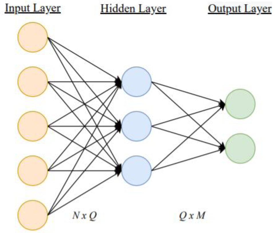
Fig. 3. Structure of an artificial neural network.
The input dataset is typically normalized prior to training the neural network for improving the learning process and convergence. For a given sample, a normalized input feature vector x is passed into the input layer of the ANN. An activation function φ transforms the ith input entry, with weights w i,j and biases b j connected to the jth output node of vector u, as shown in Eq. (9). Another activation function is applied to the hidden layer vector values to generate the prediction vector y, described by Eq. (10). This is repeated for subsequent samples to generate a set of predictions.
 $$u_j = \varphi _1\left({\mathop \sum \limits_{{\rm i\ = \ 1}}^N w_{{\rm i, j}}^1 x_i + b_j^1 } \right),$$
 $$y_k = \varphi _2\left({\mathop \sum \limits_{{\rm l\ = \ 1}}^M w_{{\rm 1, k}}^1 u_l + b_k^1 } \right).$$
The ReLU activation function, as shown in Eq. (11) and Figure 4, is commonly chosen for each layer because of its good convergence properties and reduced likelihood of reaching a vanishing gradient.
 $$\varphi ( z ) = {\max ( 0, \ }x). $$
Fig. 4. ReLU activation function.
Finally, ANNs are trained by minimizing a cost function through a back-propagation optimization algorithm. The mean squared error (MSE) function is often chosen as the cost function in regression tasks, as shown by Eq. (12). Here,  $\hat{y}$ denotes the prediction from the DR-NN and y is the labeled output.
 $${\rm MSE} = \displaystyle{1 \over n}\mathop \sum \limits_{i = 1}^n ( {y-\hat{y}} ) ^2.$$
Proposed models
The algorithm architecture in this paper combined dimensionality reduction methods with neural networks for more efficient computation and improved prediction accuracy. Specifically, PCA, PLS, and kPCA-based neural networks were constructed and compared against a standalone neural network in terms of prediction accuracy, computation time, and error uncertainty.
First, the dataset was split into training and test sets. 80% of the dataset was used for training, while the remaining 20% was reserved for testing the trained DR-NNs. Next, we split the training data into initial training and validation sets. The initial training dataset was used to fit the DR-NNs, while the validation set was used to evaluate the error of the model fit as the hyperparameters were being tuned. Finally, the test dataset was used for final evaluation of error in the trained DR-NNs.
Figure 5 shows the structure of the DR-NNs. Dimensionality reduction was applied to the raw input to reduce 16 features to a smaller set of d features. The reduced input is subsequently fed into the two layer, 64 node hidden layers to predict the final output average temperature change. The ReLU activation function was applied to each hidden layer for its good convergence behavior. For consistency, the same hidden layer structure was used in each experiment.

Fig. 5. DR-NN structure. Dimensionality reduction reduces raw input to a smaller set of input nodes.
The DR methods reduced the raw dataset to a smaller set of features, which were fed into the neural network for training. Mini-Batch Gradient Descent was selected as the optimization method for computing functional gradients based on the ANN's weights and biases. In this work, a batch size of 32 samples was used and the DR-NN weights and biases were optimized to minimize MSE. Specifically, the weights and biases were updated with every 32 training samples passed forward and back through the neural network. The training loop continued for a specified number of epochs, the number of times the entire training dataset is explored by the ANN, and a validation dataset was used for validating the model's accuracy with the optimized weights and biases.
Test case: finite element model
Experimental setup
The two-stage rolling simulation was implemented in ABAQUS/CAE using an explicit solver. The system consisted of four rollers and the workpiece as shown in Figure 6. The dimensions shown are in millimeters and were constant across all trials.

Fig. 6. Rolling simulation assembly.
The model is based on the thick bar rolling example in the ABAQUS Examples Manual v 6.12. The key differences between the model shown in Figure 6 and the benchmark example include the additional roller, additional materials, and the inclusion of adiabatic heating effects. At a room temperature of 293.15 K, the forming process was assumed to occur quickly such that the generated heat does not dissipate through the material. Thus, a dynamic, explicit analysis with the inclusion of adiabatic heating effects was conducted to obtain the change in output surface temperature. An experimental displacement control was imposed by setting the second roller at a height of 20 cm from the center of the workpiece to ensure a constant thickness output. For data generation, the python scripting feature in ABAQUS was used to iterate the input variables which affect the output temperature. The dataset was shuffled for training purposes and a total of 1095 samples were acquired for training and testing the DR-NNs.
Boundary conditions
To reduce simulation times, a quarter model was developed with symmetric boundary conditions on two planes. Two 170 mm radii rollers compress the workpiece to a thickness of 20 mm. The rotation speed of each roller is equal to the feed velocity to avoid slippage in each trial.
Material properties and design variables
Four materials were tested altogether with the material properties shown in Table 1. Table 2 shows the range of values taken by the variable inputs of the experiment. The default inelastic heat fraction value of 0.2 was used in all simulations. Steel and aluminum were chosen as their friction properties in cold rolling are well studied in the literature. The true stress versus true strain plasticity data were obtained from experiments for each material from Kopp and Dohmen (Reference Kopp and Dohmen1990), Alves et al. (Reference Alves, Nielsen and Martins2011), Deng et al. (Reference Deng, Lu, Su and Li2013), and Johnston et al. (Reference Johnston, Muha, Grandov and Rossovsky2016)
Table 1. Material properties

Table 2. Variables with range of values in the dataset

A total of 700 sample points were used for training the DR-NNs and 176 samples were used for training validation. The first roller's height range was chosen based on critical reduction ratios in cold rolling to avoid slipping. Friction in cold rolling has been shown to vary with material, feed velocity, and compression ratio (Lenard, Reference Lenard2014). Friction in cold rolling tends to decrease with feed velocity due to the time-dependent nature of adhesion bond formation. However, with sufficient roll surface roughness, friction increases with feed velocity in aluminum cold rolling (Lenard, Reference Lenard2004). In this study, we have assumed the rollers have high roughness due to the absence of lubrication in the FEA model. In general, the friction coefficient tends to decrease with reduction in low-carbon steels, regardless of lubrication. However, this behavior changes with softer materials because of reduced normal pressure during contact. Lim and Lenard (Reference Lim and Lenard1984) studied the effects of reduction ratio on friction coefficients in aluminum alloys. Their results showed that the friction coefficient increases with reduction due to a faster rate of real contact area and rate of asperity flattening.
An approximate friction model based on the combined findings in Lim and Lenard (Reference Lim and Lenard1984) and Lenard (Reference Lenard2004, Reference Lenard2014) was developed and shown in Eqs (13) and (14). Here, v denotes the feed velocity and r is the reduction ratio. The constants were determined based on best-fit curves in Microsoft Excel for Al 6061 and low-carbon steel experiments. This study assumed that steel 572 and 1018 follow the same friction model, as did Al 1050 and 2011. Furthermore, the models are only valid for steel with reduction ratios greater than 10%. Further research can be conducted to relax this assumption.
For steels (Lim and Lenard, Reference Lim and Lenard1984; Lenard, Reference Lenard2004, Reference Lenard2014):
 $$\mu = {-}\displaystyle{{0.1} \over {1300}}v + 0.0866( r ) ^{{-}0.727} + 0.082.$$
For aluminum (Lim and Lenard, Reference Lim and Lenard1984; Lenard, Reference Lenard2004, Reference Lenard2014):
 $$\mu = \displaystyle{{0.02} \over {500}}v + 0.4r + 0.13.$$
The friction models were applied as explicit general contacts in the ABAQUS rolling simulation with penalty-based properties. Overall, 16 input variables were identified: 3 geometric, 1 velocity, 2 friction measures at each roller, and 10 material properties with plasticity data found in Kopp and Dohmen (Reference Kopp and Dohmen1990), Alves et al. (Reference Alves, Nielsen and Martins2011), Deng et al. (Reference Deng, Lu, Su and Li2013), and Johnston et al. (Reference Johnston, Muha, Grandov and Rossovsky2016). Other variables such as roll surface roughness and strain rate were not included in this study.
Measurement methods and meshing
Figure 7 shows the typical output change in temperature distribution of the quarter-model workpiece after passing through both stages of the roller system.

Fig. 7. Change in temperature distribution of the quarter model.
A total of 1280 C3D8RT elements were used in the workpiece mesh and a mass scaling factor of 2758.5 was used for stabilizing the time increments. This value was chosen based on information provided in the ABAQUS Examples Manual. For this research, only the results of the central elements of the top surface were used in validating the ML models. In ABAQUS, eight elements were selected near the center of the workpiece as shown in Figure 8.

Fig. 8. Eight surface elements for average temperature on the quarter model.
The temperatures of these elements were averaged to a single value for prediction. These surface elements were chosen as measurement points because friction is prominent at the surface, the regional temperatures are similar, and mesh refinement does not significantly affect the results. We demonstrated the latter by comparing Figure 8 with a refined mesh shown in Figure 9. The difference in output temperature change is less than 1%, indicating good convergence of the FEM and validity of the selected mesh fineness.

Fig. 9. Refined mesh shows little change in results.
Results and discussion
The following dimensionality-reduced neural networks were implemented in Python 3.8.10 using the Scikit-learn library (Pedregosa et al., Reference Pedregosa, Varoquaux, Gramfort, Michel, Thirion, Grisel, Blondel, Prettenhofer, Weiss, Dubourg, Vanderplas, Passos, Cournapeau, Brucher, Perrot and Duchesnay2011) for dimensionality reduction and TensorFlow library (Abadi et al., Reference Abadi, Agarwal, Barham, Brevdo, Chen, Citro, Corrado, Davis, Dean, Devin, Ghemawat, Goodfellow, Harp, Irving, Isard, Jia, Jozefowicz, Kaiser, Manjunath, Levenberg, Mane, Monga, Moore, Olah, Schuster, Shiens, Steiner, Sutskever, Talwar, Tucker, Vanhoucke, Vasudevan, Viegas, Vinyals, Warden, Wattenberg, Wicke, Yu and Zheng2015) for regression with neural networks.
PCA-NN parameters
Figure 10 shows the results of the validation MSE after training the PCA-NN with different number of retained components. The MSE values were averaged across 40 runs. From observation, we selected seven components for the final PCA-NN reduction.

Fig. 10. PCA-NN mean squared error versus number of components retained.
PLS-NN parameters
Figure 11 shows the results of validation MSE after training the PLS-NN with different number of components retained after dimensionality reduction with PLS across 40 runs. As shown, a minimum MSE occurred with eight components, which is the number we have chosen to use in our PLS-NN model for comparison.

Fig. 11. PLS-NN mean squared error versus number of components retained.
Kernel PCA-NN parameters
In this study, we investigated radial basis functions, cosine, hyperbolic tangent, and polynomial kernels. After comparing the performance of these kernels, a cosine kernel (Ezukwoke and Zareian, Reference Ezukwoke and Zareian2019), as shown in Eq. (15), was selected in this work due to its small error convergence when combined with the neural network. Mathematically, the cosine kernel measures the similarity between two non-zero vectors where the output is the angle between them. This is equivalent to the dot product relation between two vectors and the angle between them.
 $$k( {x_i, \;\;x_j} ) = \displaystyle{{x_ix_j^T } \over {\vert {x_i} \vert \vert x_j\vert }}.$$
Figure 12 shows the results of validation MSE after training the kPCA-NN with different number of components retained after kPCA across 40 runs. For the comparison with the neural network and other DR-NNs, we chose to retain eight components based on the results of the figure above.

Fig. 12. kPCA-NN mean squared error versus number of components retained using a cosine kernel.
Training results
Table 3 shows the training hyperparameters used in each model. The DR-NN hyperparameters were selected based on the lowest converging error and the models were implemented in Visual Studio Python. The dimensionality was reduced from 16 dimensions to 8 in the DR-NNs. The computations were performed on a computer with an i7 processor with 4 cores running at 1.8 GHz on Windows 10.
Table 3. Hyperparameters in each DR-NN model

Table 4 shows a sample prediction made by each DR-NN after training. As shown, both the neural network and DR-NNs predict the temperature change with good accuracy.
Table 4. Temperature change predictions compared with FEM

Figure 13 shows the training and validation loss when fitting the DR-NNs and NN. At higher learning rates, the error does not converge to a steady global value. This is because the gradient magnitude calculated is too large and causes the weight changes to oscillate rather than converge. Furthermore, the PCA- and PLS-based neural networks improved the convergence and prediction uncertainty, showing less oscillatory behavior toward the end of the training epochs. The reduced uncertainty was also evident in the smaller whiskers and box size in the error boxplots for the PCA- and PLS-NNs compared with the neural network in Figures 14 and 15.

Fig. 13. Training and validation MSE loss for DNN and DR-NNs.

Fig. 14. MSE box plots averaged across 40 runs for DNN and DR-NNs.

Fig. 15. Computation times in seconds averaged across 40 runs for DNN and DR-NNs.
The computation times and errors below were compared against FEM results, which took 2.5 min to reach a prediction. Overall, the DR-NNs require more epochs to reach a converging error compared with the standard neural network. However, due to the lower dimensionality of the DR-NNs, the overall training times are reduced by 0.3–0.5 s, as shown in Figure 15, while maintaining comparable accuracy to the neural network, shown in Figure 14.
In total, 5300 hyperparameters, namely weights and biases, were trained in the neural network without dimensionality reduction. The number of weights and biases to be trained was reduced to 4800 in DR-NNs, requiring less storage space. Overall, both the PCA- and PLS-NNs improved upon the training time with little loss of prediction. The kPCA-NN also showed improvement in computation/training time but sacrificed much more prediction accuracy.
The DR-NNs successfully reduced the computation time, storage space, and the uncertainty in prediction error. While the prediction error in all DR-NNs were comparable to the standard neural network, the reduced computation time and storage requirements make DR-NNs a viable substitute for the lengthy FEA simulations. The complexity of the investigated cold rolling problem is low, thus the scale of time and space saved with dimensionality reduction was around 0.3–0.8 s. However, DR-NNs can be extended to high-dimensionality FEM problems involving thousands of inputs, where training the hyperparameters of full neural network can become cumbersome such as the case in imaging (Fan and Li, Reference Fan and Li2006). All in all, these methods can be applied to more complex FEA problems to give accurate assessments of output parameters in the order of seconds, compared to hours with the full simulation run.
In the future, there are improvements that can improve upon the saved computation times and storage requirements with DR-NNs. Here, we conducted trial-and-error tests to determine hyperparameters such as learning rate, batch size, and the reduced dimensionality. Optimization of the DR-NN hyperparameters can further reduce the training time and dimensionality of the problem. In terms of future work in improving the cold rolling simulation, the inclusion of parameters such as roll surface roughness and strain rate-dependent material data can yield more accurate and complex training data for assessing the DR-NNs.
Conclusion
In this paper, several dimensionality reduction techniques combined with a neural network to reduce the computation time and space required to store the trained model hyperparameters are presented. The methods were compared for predicting the output change in temperature in a two-stage cold rolling simulation. Overall, the DR-NNs successfully reduced the training time, storage space, and prediction uncertainty compared with the standalone neural network with minimal loss of accuracy. This proves the viability of using these methods to overcome the long simulation times in other FEA problems and ease the training procedure for neural networks in more complex problems.
Conflict of interest
The authors declare that they have no known competing financial interests or personal relationships that could have appeared to influence the work reported in this paper.
Acknowledgements
This work was supported by the Natural Sciences and Engineering Research Council of Canada (NSERC) under grant number RGPIN-217525.
Data availability
The data that support the findings of this study are openly available in Mendeley Data at http://doi.org/10.17632/wcp8wrdhyj.1.
Chun Kit Jeffery Hou received the BASc. Degree in Mechanical Engineering from the University of British Columbia in 2020. He is currently working toward the MASc. degree with the Advanced Research Laboratory for Multifunctional Lightweight Structures, Department of Mechanical and Industrial Engineering, University of Toronto, ON, Canada. His research interests include machine learning, finite element analysis, mechanics of materials, and failure analysis.
Dr. Kamran Behdinan (PhD) is the founding director and principal investigator of the U of T Advanced Research Laboratory for Multifunctional Lightweight Structures. His research interests include Design and Development of Light-weight Structures and Systems for biomedical, aerospace, automotive, and nuclear applications, Multidisciplinary Design Optimization of Aerospace and Automotive systems, Multi-scale Simulation of Nano-structured Materials and Composites. He has also published more than 370 peer-reviewed journal and conference papers, and 9 book chapters. He has been the recipient of many prestigious awards and recognitions such as the Research Fellow of Pratt and Whitney Canada and Fellows of the CSME, ASME, the Canadian Academy of Engineering, EIC, AAAS, as well as the Associate Fellow of AIAA.


 Open access