


1. Introduction
The breakup of a liquid stream into droplets is commonly encountered in nature and widely used in industrial applications, such as pesticide spraying, spray painting, fuel-injection systems, cooling, dispersal of biological agents and many more. In certain medical devices, such as inhalers, drug delivery is assisted by spray formation, and bubble bursting is used in breaking up kidney stones by erosion. The process of fragmentation of fluid masses, referred to as the atomization phenomenon, is mainly thought of as a consequence of the momentum difference between the liquid and the surrounding gas. This momentum difference induces a shear instability on the liquid–gas interface which forms wave structures. The liquid waves, subsequently, develop into thin liquid sheets which in turn form rims at their free end under the effect of surface tension. The liquid rims are subjected to transverse instabilities and form fingers that break into ligaments and droplets (Lasheras & Hopfinger Reference Lasheras and Hopfinger2000; Blumenthal, Hoepffner & Zaleski Reference Blumenthal, Hoepffner and Zaleski2011; Agbaglah, Josserand & Zaleski Reference Agbaglah, Josserand and Zaleski2013).
Other breakup mechanisms of liquid waves, different from the above scenario, are also observed. One instance is the droplet catapult mechanism (Jerome et al. Reference Jerome, Marty, Matas, Zaleski and Hoepffner2013) where the wave crest is stretched and forms a thin liquid sheet due to the interaction of nonlinear dynamics of the gas stream with the liquid–gas interface. Thus, the liquid sheet oscillates and breaks up into droplets. Another important breakup mechanism is the formation of holes which appear in waves prior to the formations of ligaments. The holes expand, merge with each other or with a retracting end rim and break the liquid sheet into droplets; see for instance figures 9 and 10 of Ling et al. (Reference Ling, Fuster, Zaleski and Tryggvason2017).
The formation of holes in the dynamics of thin liquid sheets is observed in many different experimental configurations. A well-known experimental case in the literature is the photographic investigation of Dombrowski & Fraser (Reference Dombrowski and Fraser1954), where the formation of holes and the importance of their collision in the destabilization of thin liquid sheets are observed. In that study, a flat sheet produced by a single-hole fan-spray nozzle is used with different liquid properties. Particularly, photographs of the flat sheet taken in a vacuum reveal the formation of holes which collide and break into droplets (see their figure 22c). Other configurations are holes formed in the bag-breakup mode of drops in the presence of a continuous air jet (Guildenbecher, López-Rivera & Sojka Reference Guildenbecher, López-Rivera and Sojka2009) or in the bursting of a soap film (Bremond & Villermaux Reference Bremond and Villermaux2005) and those observed in splashes (Marston et al. Reference Marston, Truscott, Speirs, Mansoor and Thoroddsen2016). In the case of liquid atomization, where the thickness of the dynamic liquid wave is larger compared with a soap film, these hole formation, merging and rupture have not received much attention. A recent observation of hole formation and the subsequent breakup of the liquid sheet in atomization is shown by Ling et al. (Reference Ling, Fuster, Zaleski and Tryggvason2017). One most common outcome of hole collision, which can be observed in different configurations, is the formation of a smooth or rough liquid bridge which subsequently detaches in a ligament that breaks into multiple drops or collapses into a single large drop. Even though the physical mechanisms responsible for hole formation are not well understood, the fate of the detached ligament, itself, is known to depend on its aspect ratio and the associated Ohnesorge number (Schulkes Reference Schulkes1996; Castrejón-Pita, Castrejón-Pita & Hutchings Reference Castrejón-Pita, Castrejón-Pita and Hutchings2012; Driessen et al. Reference Driessen, Jeurissen, Wijshoff, Toschi and Lohse2013; Hoepffner & Paré Reference Hoepffner and Paré2013). It appears thus crucial to investigate the mechanisms leading to ligament formation in the case of the collision of holes and the resulting ligament characteristics.
In the case of a single hole formed in a thin liquid sheet at rest, the hole can either collapse or expand depending on the size of its diameter compared to the liquid sheet thickness (Taylor & Michael Reference Taylor and Michael1973; Moriarty & Schwartz Reference Moriarty and Schwartz1993; Debrégeas, de Gennes & Brochard-Wyart Reference Debrégeas, de Gennes and Brochard-Wyart1998). At the hole free end, capillary forces are no longer balanced and the hole edge retracts and forms a rim. The rim grows linearly in time with a velocity that rapidly reaches the so-called Taylor–Culick velocity,  ${V_{TC}}=\sqrt {2\sigma /\rho e}$, when the viscous effects are small (Taylor Reference Taylor1959; Culick Reference Culick1960). Here, $\sigma$ represents the surface tension, $\rho$ the density of the liquid and $e$ the thickness of the liquid sheet.
In this paper, we focus on the simplified case of a flat and static liquid sheet. We study the merging process of two distinct holes and a single hole with a straight end rim, using three-dimensional numerical simulations. Realistic liquid–gas conditions, namely the air/water system, are used and the considered thicknesses of the thin liquid sheet are similar to those formed in liquid atomization processes. The liquid sheet and the surrounding gas are at rest in this study. We aim at a comprehensive understanding of the process of drop formation from hole–hole and hole–rim merging.
2. Numerical method and preliminary simulations
We simulate a liquid–gas system with respective densities  $\rho _g$ and $\rho _l$ and viscosities $\mu _g$ and $\mu _l$ using the one-fluid approach of the incompressible Navier–Stokes equations:
 \begin{gather} \rho (\partial_t \boldsymbol{u}+\boldsymbol{u} \boldsymbol{\cdot} {\boldsymbol{\nabla}} \boldsymbol{u}) = - {\boldsymbol{\nabla}} p + {\boldsymbol{\nabla}} \boldsymbol{\cdot} (2\mu \boldsymbol{\mathsf{D}}) + \gamma \kappa \delta_s \boldsymbol{n}, \end{gather}
 \begin{gather}{\boldsymbol{\nabla}} \boldsymbol{\cdot} \boldsymbol{u}= 0, \end{gather}
where  $\boldsymbol {u}$ is the fluid velocity, $\rho \equiv \rho (\boldsymbol {x}, t)$ is the density, $\mu \equiv \mu (\boldsymbol {x}, t)$ is the viscosity and $\boldsymbol{\mathsf{D}}$ is the deformation tensor. The Dirac distribution function $\delta _s$ expresses the fact that the surface tension term is concentrated at the interface, $\kappa$ and $\boldsymbol {n}$ being the curvature and the normal of the interface, respectively. We use the Basilisk code (Popinet Reference Popinet2018), an improved numerical solver based on Gerris, that has been validated for a number of multiphase flow problems (Fuster et al. Reference Fuster, Agbaglah, Josserand, Popinet and Zaleski2009; Agbaglah et al. Reference Agbaglah, Delaux, Fuster, Hoepffner, Josserand, Popinet, Ray, Scardovelli and Zaleski2011, Reference Agbaglah, Thoraval, Thoroddsen, Zhang, Fezzaa and Deegan2015). Basilisk is an open-source code where the interface is tracked using a volume-of-fluid method on an octree structured grid allowing adaptive mesh refinement. The incompressibility condition is satisfied using a multigrid solver described in detail in Popinet (Reference Popinet2003, Reference Popinet2009). The calculation of the surface tension is based on the balanced-force technique (Francois et al. Reference Francois, Cummins, Dendy, Kothe, Sicilian and Williams2006) and the mesh is refined/coarsed based on a criterion of wavelet-estimated discretization error (van Hooft et al. Reference van Hooft, Popinet, van Heerwaarden, van der Linden, de Roode and van de Wiel2018).
Preliminary simulations of the hole expansion in a thin liquid sheet and the end rim retraction of a bounded liquid sheet are performed using liquid and gas properties described in table 1, which correspond to the air/water configuration. As recently shown in a quasi-planar liquid–gas atomization (Ling et al. Reference Ling, Fuster, Zaleski and Tryggvason2017), the minimum thickness of the formed liquid sheet, after being stretched by the surrounding fast gas stream, is between  $25$ and $50\ \mathrm {\mu }\textrm {m}$ corresponding to an Ohnesorge number (the ratio of viscous forces to surface tension) $Oh=\mu _l/\sqrt {\rho _l\sigma e_0}\approx 0.02$.
Table 1. Simulation parameters.

In our numerical simulations, the thickness of the flat liquid sheet is set to  $e_0=25\ \mathrm {\mu }\textrm {m}$ with a corresponding ${Oh}=0.017$. The computational domain corresponds to $100e_0\times 100e_0\times 100e_0$ and is discretized with an adaptive mesh up to a maximum number of $2^9$ grid points along each dimension, corresponding to a minimum mesh size $\varDelta =e_0/6$ and 134 million cells if a uniform grid was used. Note that a similar mesh size has been used in previous two-dimensional simulations of a retracting liquid sheet (see, for example, Fuster et al. (Reference Fuster, Agbaglah, Josserand, Popinet and Zaleski2009) and Gordillo et al. (Reference Gordillo, Agbaglah, Duchemin and Josserand2011) where the retraction features were accurately captured). The origin of the reference frame is set at the middle of the computational domain and the $x$,
$x$,  $y$ and $z$ axes, where the $x$ and $z$ axes represent horizontal directions and the $y$ axis represents the vertical direction, are shown in figure 1. Symmetry boundary conditions are applied on the edges of the domain. For the hole expansion simulation, an initial hole of diameter $D_0=2e_0$ and centre placed in the middle of the liquid sheet is considered, while for the straight end rim retraction a longitudinal length of $88e_0$ with a round bounded edge of diameter
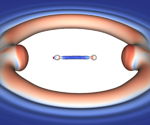
  $e_0$ is used.The preliminary simulations are used to compare the dynamics of the free ends of the opening hole and the bounded liquid sheet. As shown in figures 1(a) and 1(b) a toroidal rim is formed at the free end of the hole while a straight rim is formed at the free end of the bounded liquid sheet, respectively. Both rims retract due to surface tension and after a short transient reach a quasi-stationary regime with a constant velocity, where most of the dynamics consists of a slow increase of the rim size. We refer to this stage as the Taylor–Culick regime. By considering the rim circular, an assumption that strongly depends on the Ohnesorge number (Gordillo et al. Reference Gordillo, Agbaglah, Duchemin and Josserand2011), a simple mass balance yields a square root of time evolution of the rim radius. Figure 2(a) shows the square of the non-dimensional rim radius $r/r_0$, where $r_0=e_0/2$, as a function of the non-dimensional time $t/\tau _0$, where $\tau _0=\sqrt {\rho _l e_0^3/\sigma }$. After a transient stage, the square of the rim radius obtained in the simulations grows linearly in time as expected. However, the straight rim formed at the free end of the bounded liquid sheet grows rapidly compared with the toroidal rim formed at the free end of the opening hole. We attribute this difference to a geometrical effect since the toroidal rim velocity has both non-zero longitudinal and transverse components and therefore accumulates less liquid than the straight rim. On the other hand, for both cases the velocity norm reaches the same constant value after the transient stage (see figure 2b). The obtained constant retraction speed is $7\,\%$ smaller than the predicted Taylor–Culick velocity. This small discrepancy can be explained by the considered $Oh$ value and the large density and viscosity ratios which can alter the speed at which the edge is pulled back; see for instance Song & Tryggvason (Reference Song and Tryggvason1999), where a difference of approximately $12\,\%$ was obtained when varying the density and viscosity ratios.

Figure 1. (a) Hole expansion in a thin liquid sheet, with the formation of a toroidal rim at the free end of the hole. The initial diameter of the hole is  $D_0 = 2e_0$, where $e_0$ represents the thickness of the liquid sheet. (b) Straight end rim formation and retraction in a bounded thin liquid sheet. The colours show the velocity norm rescaled by ${V_{TC}}$, with blue colour corresponding to 0 and red colour to 1.

Figure 2. Comparison of toroidal (red colour) and straight (blue colour) rim retraction. (a) Square of the liquid rim radius as a function of the non-dimensional time. The black dashed lines correspond to linear fits. (b) Rim retraction velocity norm as a function of the non-dimensional time. The black dashed line corresponds to the value 0.93.
It is noteworthy that no transverse corrugations, similar to those leading to the formation of liquid fingers (Agbaglah et al. Reference Agbaglah, Josserand and Zaleski2013; Agbaglah & Deegan Reference Agbaglah and Deegan2014), are developed in the end rim dynamics described above. This is similar to the observed stable regime of Fullana & Zaleski (Reference Fullana and Zaleski1999). Indeed, a stable rim dynamics is expected since no initial rim acceleration is prescribed and the initial thickness of the liquid sheet scaled by the initial rim size is high,  $e_0/r_0=2$, as predicted by the linear theory of Agbaglah et al. (Reference Agbaglah, Josserand and Zaleski2013).
The difference in the size of the end rims of the opening hole and the bounded liquid sheet can result in non-symmetric contributions in their merging process. In the next section, we concentrate on the differences in the merging process of two distinct toroidal rims and the merging of a straight rim with a toroidal one.
3. Hole–hole and hole–rim merging processes in a thin liquid sheet
Three-dimensional computations of the merging dynamics of a toroidal rim and a straight rim are performed. Two different cases are considered: hole–hole merging (see figure 3a), which corresponds to the dynamics of two different holes in a thin liquid sheet; and hole–rim merging, corresponding to a single hole in a bounded thin liquid sheet (see figure 3b). The considered thickness of the liquid sheet is the same as in the above simulations,  $e_0=25\ \mathrm {\mu }\textrm {m}$, and the same liquid–gas properties as in table 1 are used. The diameter of the holes is set to $2e_0$. For the hole–hole computations, the two holes are positioned around the centre of the liquid sheet and the distance between the centres of the two holes corresponds to $10e_0$. For the hole–rim case, the centre of the hole is placed at a distance of $10e_0$ from the free edge of the bounded liquid sheet. Note that this small distance between the two adjacent holes or between the hole and the free edge is chosen in order to mimic close hole collisions observed in atomization processes (Ling et al. Reference Ling, Fuster, Zaleski and Tryggvason2017). It is noteworthy that for viscous flow (large ${Oh}$) the rim velocity may vary so that a different distance could trigger a merging process different from the one presented herein. Figure 3(a,b) displays the time sequences showing the dynamics of the hole expansion and merging processes (see supplementary movies for the same sequence available at https://doi.org/10.1017/jfm.2020.1016). For both hole–hole and hole–rim simulations, the holes expand, form rims at their free ends and merge each other or with the straight rim in the case of the bounded liquid sheet. A quasi-symmetric liquid bridge, connecting the two holes or the hole and the straight rim, is formed after the merging (see the third image in each of figures 3a and 3b). Next, the liquid bridge stretches in time, as the resulting hole after the merging continues to grow, and subsequently detaches into a ligament with blobs formed at its tips. The ligament can either break into droplets or recoil to form a single droplet as shown later in figures 10 and 11.

Figure 3. Time sequences of hole–hole merging (a) and hole–rim merging (b). From left to right and top to bottom the corresponding times  $t/\tau _0$ are 0, 1.6, 4.1, 5.8, 6.6, 9.1, 14.1, 16.6 for the hole–hole case (a) and 0, 1.6, 5, 6.6, 9.1, 10.8, 25, 28.3 for the hole–rim case (b) (see also the supplementary movies for the same sequence).
The size of the rims at the onset of the merging of the two holes and the hole with the edge of the bounded liquid sheet is shown in figure 4(a) where a vertical slice (in the  $y$ direction), in the mid-plane of the liquid sheet, is displayed. As expected, based on the preliminary simulations above, the size of the rims is the same for the hole–hole case while for the hole–rim the size of the straight rim is larger than that of the toroidal rim. As shown in figure 4(b,c), which presents horizontal slices (top view, in the $x$–
$x$– $z$ plane), the liquid bridge stays straight in the case of hole–hole merging while it is curved outward in hole–rim merging. This is a consequence of the difference in the shape and size of the toroidal rim and the straight rim for the hole–rim case. In fact, the straight rim has only one principal curvature that is smaller than that of the toroidal rim. Therefore, at merging, the toroidal rim has a larger capillary pressure compared with the straight rim, resulting in the outward curved shape of the liquid bridge.

Figure 4. Two-dimensional slices showing the size of the rims (a) for the hole–hole case (red colour) and the hole–rim case (blue colour), the formed liquid bridge and the resulting hole after the merging for the hole–hole (b) and the hole–rim (c) cases. Parameters  $d_h$ and $l$ represent the horizontal diameter and the length of the liquid bridge, respectively.
A closeup view of the resulting rims after merging reveals the oscillation of the liquid bridge diameter in the horizontal ( $x$ or $z$ axis) and the vertical ( $y$ axis) directions (see the time sequence images in figure 5a,b). This oscillation is described as follows. The liquid bridge deforms in the vertical direction ( $y$ axis) after the collision of the rims bounding the two holes or the liquid sheet, and forms a vertically expanding free liquid sheet. The kinetic energy of the free liquid sheet decreases and dissipates over time. Subsequently, the upper and lower edges of the vertically expanded liquid bridge (see figure 5 $a1{,}b1$) recede under capillary forces and merge. The liquid bridge, thereafter, deforms in the horizontal direction and forms a horizontally expanding free liquid sheet (see figure 5 $a3{,}b3$), which also will recede and merge again. The oscillation of the liquid bridge has the consequence of sucking liquid from the central part of the bridge into its ends, which thus forms a cone that gets thicker with time. These oscillation sequences are similar to the phases observed in the case of the collision of two liquid droplets (e.g. Qian & Law Reference Qian and Law1997; Brenn & Kolobaric Reference Brenn and Kolobaric2006). The dynamics of the liquid bridge is therefore subjected to three different motions: the oscillation of its diameter, the mid-plane contraction and the stretching or elongation. These three motions are next examined for the two considered cases, hole–hole and hole–rim merging.

Figure 5. Time sequence showing the liquid bridge oscillation by zooming in on the resulting rims after merging (shown in a perspective view). The corresponding times  $t/\tau _0$ are 4.2, 5, 5.8, 6.2, 6.5 for the hole–hole case (a) and 5, 6.7, 6.5, 7.5, 9.2 for the hole–rim case (b).
We measure the horizontal and vertical mid-plane diameters of the liquid bridge, denoted by  $d_h$ and $d_v$, respectively, and the diameter of the resulting hole after merging, denoted by $l$ (also considered as the length of the liquid bridge; see figure 4b,c). The obtained results are shown in figures 6(a) and 6(b) for the hole–hole and the hole–rim simulations, respectively, where $d_h$ and $d_v$ are plotted as a function of the non-dimensional time before breakup $(t-t_b)/\tau _0$, $t_b$ representing the liquid bridge pinch-off time. The time evolution of $d_h$ and $d_v$ resembles an under-damped oscillatory system as in the case of a mass–spring system but with a period that decreases with time.The amplitude of the oscillation is obtained by recording the maximum vertical deformation ${d_v}_{max}$ for each period of the oscillations. A decaying exponential evolution of the amplitude is obtained for both the hole–hole and hole–rim cases as shown in figure 7(a). However, as shown in this figure, the range of the exponential decay is less than one order of magnitude due to the involved short time scale of the breakup process. It is worth noticing that the initial vertical deformation of the liquid bridge is larger for the hole–rim case than for the hole–hole case due to the above-mentioned non-symmetric size of the rims at merging. Nevertheless, the amplitude of the liquid bridge oscillation decays more rapidly in the hole–hole case. This is a consequence of the rapid elongation of the liquid bridge in the case of hole–hole merging, as will be discussed later. Halfway up the vertical or horizontal expansion, the central part of the liquid bridge takes a cylindrical shape with a diameter $d$ that decreases with time. The diameter $d$ is obtained when ${d_h}={d_v}=d$. As shown in figure 7(b), $d$ decreases linearly with time for the hole–rim case while a quadratic decrease with time is observed for hole–hole merging. The length of the liquid bridge $l$ is shown in figure 8(a) for hole–hole and hole–rim merging. While $l$ grows linearly with time for the hole–hole case, the slope of the elongation is lower for hole–rim merging and even decreases after a certain non-dimensional time. This indicates that the resulting hole after merging continues to expand with a constant speed in the hole–hole case while its expansion is slower and decreases in time for the hole–rim case. This slower expansion can be attributed to the opposite motion of the straight rim and the hole. Following the study of a stretched liquid ligament (Marmottant & Villermaux Reference Marmottant and Villermaux2004), we compare the bridge extension rate $1/\tau _e=(\textrm {d}l/\textrm {d}t)/l$ with the capillary contraction rate $1/\tau _c=\sqrt {\sigma _l/(\rho _l d^3)}$. The ratio of the extension rate to the capillary contraction rate $(1/\tau _e)/(1/\tau _c)=\tau _c/\tau _e$ is shown in figure 8(b) as a function of the non-dimensional time. For both hole–hole and hole–rim merging this ratio is smaller than 1 and corresponds to the slow extension limit of Marmottant & Villermaux (Reference Marmottant and Villermaux2004). However, the dynamics of the liquid bridge, shown in figures 3, 10 and 11, differs from this observed in the slow extension limit of the stretched ligament, where the oscillation motion described above was not present. Indeed, the liquid cones formed at the bridge ends, in the present study, are thicker and the central part of the bridge forms a cylindrical ligament similar to the columnar shape observed rather in the rapid extension limit of the stretched liquid ligament (Marmottant & Villermaux Reference Marmottant and Villermaux2004). In addition, the liquid bridge does not break up by capillary contraction on a single point (as in the slow extension limit) but pinches off on two symmetric points connecting the central cylindrical part to the cones similarly to the pinch-off of a symmetric film bridging two circles (Cryer & Steen Reference Cryer and Steen1992; Chen & Steen Reference Chen and Steen1997). The oscillation motion thus has the effect of damping the capillary contraction.

Figure 6. Mid-plane vertical diameter  $d_v$ and horizontal diameter $d_h$ as a function of the non-dimensional time before breakup for the hole–hole case (a) (with $d_v$ shown in red colour and $d_h$ in grey colour) and the hole–rim case (b) (with $d_v$ shown in blue colour and $d_h$ in green colour). The open square in (a) (and open circle in b) shows the diameter of the mid-plane circular shape, $d_h=d_v$, of the bridge and the filled square in (a) (and filled circle in b) shows the amplitude of $d_v$.

Figure 7. (a) Amplitude of the vertical deformation of the liquid bridge,  $d_{v_{max}}$, as a function of the non-dimensional time before breakup for the hole–hole (red square) and the hole–rim (blue circle) cases. The blue and red lines represent exponential fits. (b) Mid-plane circular shape diameter, $d=d_h=d_v$, for the hole–hole case (red square with the red line corresponding to a parabolic fit) and for the hole–rim case (blue circle with the blue line corresponding to a linear fit).

Figure 8. (a) Length of the liquid bridge,  $l$, as a function of the non-dimensional time for the hole–hole case (red square) and the hole–rim case (blue circle). (b) Ratio of the extension rate to the capillary contraction rate for the hole–hole case (red square) and the hole–rim case (blue circle).
Next, the minimum horizontal diameter (in the  $x$–
$x$– $z$ plane) along the liquid bridge, denoted by $d_{min}$, is compared with the mid-plane diameter $d_h$ for the hole–rim case (a similar comparison is obtained for the hole–hole case but not shown herein). As shown in figure 9, where $d_{min}$ is plotted as a function of the non-dimensional time before breakup, the minimum diameter location changes along the liquid bridge. Far from the liquid bridge pinch-off time, the minimum diameter location varies between the mid-plane and the plane of a local minimum induced by the folding which results from the bridge oscillation (see figure 5b). Thereafter, $d_{min}$ is located in the mid-plane when the amplitude of the oscillation and the size of the liquid bridge have decreased enough so that no folding could be observed. Finally, close to the pinch-off time, the minimum diameter switches from the mid-plane to the plane of a point connecting the central cylindrical part to the cone, where the breakup is observed. As shown by the inset plot of figure 9, close to the pinch-off time, a reasonable agreement is obtained with the inviscid theory, $d_{min}\sim (t_b-t)^{2/3}$ (Peregrine, Shoker & Symon Reference Peregrine, Shoker and Symon1990; Eggers Reference Eggers1997; Eggers & Villermaux Reference Eggers and Villermaux2008).

Figure 9. Minimum diameter  $d_{min}$ (blue circle) along the liquid bridge compared with the mid-plane diameter $d_h$ (blue line). Images of the hole–rim simulation are also shown to indicate the minimum diameter location along the liquid bridge. The inset displays the comparison of $d_{min}$, close to the pinch-off time, and the function $0.68(t_b-t)^{2/3}$ (black line).
Figures 10 and 11 show the liquid bridge pinch-off and the subsequent dynamics of the formed ligament for hole–hole and hole–rim merging, respectively. It is worth noticing that for both cases the amplitude of the oscillation of the bridge vanished completely prior to the pinch-off. Three different computations, using different liquid sheet thicknesses, namely  $e_0$, $2e_0$ and $4e_0$, are displayed in figures 10 and 11. The so-called end-pinching mechanism (Stone, Bentley & Leal Reference Stone, Bentley and Leal1986) is observed. Here, the bulbous ends of the contracting ligament can either pinch off in daughter drops (see figures 10a and 11a) or remain attached, recoil and form a single drop when capillary forces are not large enough to overcome viscous forces (see figures 10b,c and 11b,c). For the smaller liquid sheet thickness, $e_0$, the liquid bridge presents surface undulations due to evolving capillary waves on the surface of the ligament (see figures 10a and 11a).The initial aspect ratio of the ligament, $l/d$, after the liquid bridge detaches and the associated Ohnesorge number, ${Oh}_l=\mu _l/\sqrt {\rho _l\sigma (d/2)}$, are known to control the end-pinching processes (Schulkes Reference Schulkes1996; Notz & Basaran Reference Notz and Basaran2004; Castrejón-Pita et al. Reference Castrejón-Pita, Castrejón-Pita and Hutchings2012; Driessen et al. Reference Driessen, Jeurissen, Wijshoff, Toschi and Lohse2013; Hoepffner & Paré Reference Hoepffner and Paré2013). These two parameters are calculated for six different numerical simulations (with liquid sheet thicknesses ranging from $e_0$ to $6e_0$) and shown in figure 12(a). The obtained ${Oh}$ values are between $2\times 10^{-2}$ and $4\times 10^{-2}$. For these ${Oh}$ limits, the critical initial aspect ratio below which the ligament does not break is $17.5\pm 2.5$ (see table 3 of Notz & Basaran (Reference Notz and Basaran2004)). This is consistent with the present simulations where end pinching is observed only for the lower liquid sheet thickness (see figures 10a and 11a) for which the ligament initial aspect ratio is larger than 22. Figure 12(b) shows the obtained volume-based drop diameter as a function of the liquid sheet thickness. The drop diameter is averaged in the case of the liquid sheet thickness $e_0$ where multiple daughter drops are generated. The drop size increases with the liquid sheet thickness and is slightly smaller for the hole–hole case. In the cases where the ligament does not break ( $e/e_0\geq 2$), the volume of the drop is the same as the volume of the detached ligament and a power-law increase is observed in figure 12(b). By using a least-squares fit, we obtained that $d_{drop}\sim e^{0.47}$ for the hole–rim case while $d_{drop}\sim e^{0.35}$ for the hole–hole case. Nevertheless, it should be noted that the power-law fitting range of the generated drop diameters is smaller than one order of magnitude for simulations presented herein with liquid sheet thicknesses between $25$ and $150\ \mathrm {\mu }\textrm {m}$.

Figure 10. Pinch-off of the liquid bridge and subsequent dynamics of the ligament for hole–hole merging. (a) A liquid sheet thickness  $e_0$ and non-dimensional times 15, 15.8 and 25 (from left to right). (b) A liquid sheet thickness $2e_0$ and non-dimensional times 21.6, 25 and 33.3 (from left to right). (c) A liquid sheet thickness $4e_0$ and non-dimensional times 33.3, 36.6 and 46.6 (from left to right).

Figure 11. Pinch-off of the liquid bridge and subsequent dynamics of the ligament for hole–rim merging. (a) A liquid sheet thickness  $e_0$ and non-dimensional times 25, 26.6 and 33.3 (from left to right). (b) A liquid sheet thickness $2e_0$ and non-dimensional times 33.3, 35.8 and 40.8 (from left to right). (c) A liquid sheet thickness $4e_0$ and non-dimensional times 53.3, 56.6 and 65 (from left to right).

Figure 12. (a) Initial aspect ratio of the ligament (solid lines) and the associated Ohnesorge number  $Oh_l$ (dashed lines) as a function of the liquid sheet thickness for the hole–hole case (red square) and the hole–rim case (blue circle). (b) Mean diameter of the formed drops as a function of the liquid sheet thickness for the hole–hole case (red square) and the hole–rim case (blue circle). The blue line represents the power-law fit $2.484\times (e/e_0)^{0.47}$ while the red line represents $2.74\times (e/e_0)^{0.35}$.
4. Discussion and conclusion
Three-dimensional numerical simulations of the merging process of two distinct holes, referred to as the hole–hole case, and a hole with a straight rim, referred to as the hole–rim case, are presented using different liquid sheet thicknesses ranging from  $e_0=25\ \mathrm {\mu }\textrm {m}$ to $e=6e_0=150\ \mathrm {\mu }\textrm {m}$, which correspond to liquid sheet thicknesses obtained in liquid–gas atomization (Ling et al. Reference Ling, Fuster, Zaleski and Tryggvason2017). The simplified case of a static liquid–gas flow is considered. The computations are performed using the realistic air/water conditions and preliminary simulations of a single hole expansion and the dynamics of the rim formed at the free end of a bounded liquid sheet have shown good agreement with Taylor–Culick predictions (Taylor Reference Taylor1959; Culick Reference Culick1960).
A liquid bridge is formed after the merging of the two holes or the hole and the straight rim. The dynamics of the liquid bridge is subjected to three different motions: the vertical and horizontal oscillations of its diameter, which resemble a mass–spring system but with a period that decreases in time; the mid-plane contraction; and the liquid bridge elongation. Halfway up the vertical or horizontal expansion, the central part of the liquid bridge takes a cylindrical shape with a diameter that decreases linearly with time for the hole–rim case, while a faster quadratic decrease is observed for the hole–hole case.
Thereafter, the amplitude of the bridge diameter oscillation decreases exponentially and vanishes. Thus, the central part of the liquid bridge remains cylindrical. While this cylindrical shape of the liquid bridge resembles the columnar shape observed in the rapid extension limit of a stretched liquid ligament (Marmottant & Villermaux Reference Marmottant and Villermaux2004), analysis of the ratio of the extension rate to the capillary contraction rate reveals a ratio smaller than 1 for both the hole–hole and the hole–rim cases, which instead indicates a slow extension regime. The oscillation motion, not present in the stretched liquid ligament study of Marmottant & Villermaux (Reference Marmottant and Villermaux2004), has the effect of sucking liquid from the central part of the bridge into its ends, which form cones that get thicker with time. Consequently, the central part of the liquid bridge is subjected to a local stretching which leads to the rapid decrease of the ligament diameter and precludes the local capillary contraction and the single-point pinch-off observed in the slow extension limit.
Later, the liquid bridge pinches off on two symmetric points connecting the central cylindrical part to the cones and forms a contracting ligament with bulbous ends which can either detach according to the end-pinching mechanism or recoil and merge into a single large drop, depending on the ligament initial aspect ratio and the associated Ohnesorge number. In the case where the ligament does not break ( $e/e_0\geq 2$), the volume-based diameter of the formed drop is shown to increase as a power-law function of the liquid sheet thickness. The obtained power-law exponents correspond to 0.47 for the hole–rim case and 0.35 for the hole–hole case.
The dynamics of the hole–hole and the hole–rim merging shown herein do not exhibit any marked destabilization of the rims bounding the adjacent holes. No formation of liquid fingers is obtained even though some transverse corrugations of the rim are observed (see for instance the last image in figure 3b). Here, the holes expand steadily after a short transient while in some experimental configurations, such as the bag-breakup mode of drops or in atomization processes, they are accelerated by a fast gas stream. However, the stable dynamics of the bounding rims of the holes obtained herein agrees with the conclusion of Dombrowski & Fraser (Reference Dombrowski and Fraser1954) where a regular process with no disintegration of the rims is obtained for a steadily expanding liquid sheet (see for instance their figure 28c). It is also noteworthy that small values of the Ohnesorge number, of the order of  $10^{-2}$, are obtained for the detached ligament in our calculation. A greater value could be achieved with a more viscous fluid, compared with the water conditions used herein. The ligament may break up into more droplets by a mechanism such as the Rayleigh–Plateau instability, in a case where the associated Ohnesorge number is close to or greater than $10^{-1}$ (Driessen et al. Reference Driessen, Jeurissen, Wijshoff, Toschi and Lohse2013).
Supplementary movies
Supplementary movies are available at https://doi.org/10.1017/jfm.2020.1016.
Acknowledgements
The author thanks Wayne State University for support through the start-up fund and for computational support.
Declaration of interests
The author reports no conflict of interest.


 Open access