


Introduction
Radio-echo sounding (RES) is used to measure ice thickness and basal topography of ice sheets and glaciers, with measurements dating back to 1960, and internal stratigraphy in the echograms has been seen for nearly as long (Reference Robin, Evans and BaileyRobin and others, 1969; Reference GudmandsenGudmandsen, 1975). The internal reflecting horizons (IRHs) are generally accepted to be isochrones (Reference SiegertSiegert 1999; Reference Hempel, Thyssen, Gundestrup and ClausenHempel and others, 2000) and can, in some parts of the ice sheet, span several hundred kilometers in Greenland and several thousand kilometers in Antartica (Reference Steinhage, Kipfstuhl, Nixdorf and NixdorfSteinhage and others, 2013). In this paper, we refer to the IRHs as internal layers. Ice cores from the Greenland ice sheet are an archive of past climate, dating back up to 128.5 ka (NEEM Community Members, 2013); however, these cores represent point measurements on the vast ice sheet. The internal layers can be cross-linked with the high-resolution ice-core record to provide a better understanding of the internal ice-sheet dynamics and changes to mass balance (Reference Welch and JacobelWelch and Jacobel, 2003). The internal layers vary in depth and intensity; sometimes they even disappear and then reappear. The depth variability is caused by changes in accumulation (Reference Baldwin, Bamber, Payne and LayberryBaldwin and others, 2003), ice flow (Reference Vaughan, Corr, Doake and WaddingtonVaughan and others, 1999) and bedrock melt (Reference Fahnestock, Abdalati, Luo and LuoFahnestock and others, 2001), and the layer depth conversion from the two-way travel time of the radar wave is influenced by the firn density profile (Reference Kovacs, Gow and MoreyKovacs and others, 1995). Intensity variations caused by the limitations of the radar, including focusing and slope effects, have been described by Reference HarrisonHarrison (1971) and Reference Jacobel and HodgeJacobel and Hodge (1995). Other intensity variations are caused by physical features, such as attenuation from surface melt (Reference ForsterForster and others, 2014) and crevasses (Reference Gades, Raymond, Conway and JacobelGades and others, 2000), or events during the acquisition, such as plane turns.
Manually picking internal layers is very time-consuming. Reference Sime, Hindmarsh and CorrSime and others (2011) estimated that tracing 20 layers in a 20 000km RES survey would require 10 operator-years to complete. To reduce the manual workload, both commercially available software and custom-developed methods have been used to trace layers.
Commercial software originally developed for processing seismic datasets has been re-purposed into tracing RES layers: Landmark OpenWorks (used by, e.g., Reference Eisen, Nixdorf, Wilhelms and WilhelmsEisen and others, 2004; Reference Rotschky, Eisen, Wilhelms, Nixdorf and NixdorfRotschky and others, 2004) and ReflexW by Sandmeier Scientific (used by, e.g., Reference Karlsson, Rippin, Vaughan and CorrKarlsson and others, 2009; Reference MottramMottram and others, 2009). The underlying tracking algorithms are not published, but the ReflexW 4.0 user manual says that the layer tracing is based on phase tracking and peak-following, and Reference Eisen, Nixdorf, Wilhelms and WilhelmsEisen and others (2004) describe the operation of OpenWorks also as peak-following. Commercial software seems adequate to trace layers in specific studies, but the solutions leave no room for improvement or analysis of the tracing algorithms. The software also locks access to the algorithm such that specific format conversions might be needed to incorporate it into a processing workflow.
A number of tailored methods have been developed to extract features from RES echograms: Reference Crandall, Fox and PadenCrandall and others (2012) used probabilistic scene labeling to detect the air–ice and ice–bedrock interface of echograms, Reference Karlsson, Dahl-Jensen, Gogineni and PadenKarlsson and others (2013) fitted a ramp function to detect a climatic transition, and Reference Fahnestock, Abdalati, Luo and LuoFahnestock and others (2001) and Reference Baldwin, Bamber, Payne and LayberryBaldwin and others (2003) traced layers using iterative peak-following and pattern matching.
One of the key challenges in constructing an automated tracking method for RES is the fact that in some regions the layers are closely spaced. This creates many identical, slightly offset, layer candidates, and if the algorithm chooses the wrong candidate, then it could divert into the neighboring layers.
Most of the layer-tracking methods referenced above use a peak-following scheme, which makes them liable to steer into neighboring layers in regions where the visible stratigraphy deteriorates. Instead of propagating the traced layer along the track, as these schemes do, a method that traces the layer by optimizing the position of the entire layer is preferable, as that could bridge areas with poor echogram quality.
The estimated slope of the layers can be used to form synthetic isochrones. ReflexW uses the phase of the reflected wave to infer the slope and steer the layer trace. One method for deriving layer slope from RES echogram intensity has been presented by Reference Sime, Hindmarsh and CorrSime and others (2011), a multi-step procedure where the layer slope is inferred from measurements on segmented layer objects.
Here we present two new automated methods: (1) a simplified method for inferring the local layer slope, which can be used to create initial estimates of layer positions; and (2) a method for tracking a layer from that initial estimate. An iterative optimization technique, known as an active contour model or snake, is used to fit the layer estimate to the echogram, while preserving smooth layers and minimizing accidental jumps to adjacent layers. The combined process is not completely autonomous, as a human operator is required to pick seed points for the initial layer estimates.
Data
For this study a sample dataset was chosen from the Center for Remote Sensing of Ice Sheets (CReSIS, University of Kansas, USA) data archive (Reference GogineniGogineni, 2012), which is also available from the US National Snow and Ice Data Center (Reference LeuschenLeuschen, 2011). The dataset covers a 423 km transect along the ice divide in northern Greenland (Fig. 1), from the North Greenland Ice Core Project (NGRIP) ice core (75.018 N, 42.538 W; NorthGRIP Members, 2004) to the North Greenland Eemian Ice Drilling (NEEM) ice core (77.458 N, 51.068 W; NEEM Community Members, 2013). It was obtained on 6 May 2011 using the Multichannel Coherent Radar Depth Sounder/Imager (MCoRDS/I; Reference Rodriguez-MoralesRodriguez-Morales and others, 2014) on a NASA P-3 Orion aircraft during the 2011 Arctic Operation IceBridge Mission (Reference Koenig, Martin, Studinger and StudingerKoenig and others, 2010). The radar was operated with a chirp signal from 180 to 210 MHz. After processing, the average horizontal resolution is 13 m, and the vertical range resolution is 2.8 m, assuming a constant dielectric permittivity of є' r = 3:15 (Reference KohKoh, 1992; Reference Kovacs, Gow and MoreyKovacs and others, 1995).
Fig. 1. The 423 km flight line from NGRIP to NEEM in northern Greenland.
A correction for higher wave velocity in the lower-density firn was applied for the two-way travel time to depth conversions using a constant offset at each drill site. Manual bedrock picks were made at both drill sites. The offset was found from the difference between the length of the ice core and the distance to bedrock assuming a constant wave velocity of c/√є'r , where c is the velocity of light in air. We found the firn corrections to be 15.8 m for the NEEM site and 8.7 m for the NGRIP site, which is comparable to firn corrections used at the Greenland Ice Core Project (GRIP) drill site (Reference Hempel, Thyssen, Gundestrup and ClausenHempel and others, 2000).
The NEEM ice-core depth-age profile has been matched to the NGRIP core profile using match points from electrical conductivity measurements (ECM) (Reference RasmussenRasmussen and others, 2013). These depth-depth match points were used as ground truth for evaluating the quality of automatically traced layers. Both depth-age profiles of NGRIP and NEEM were extended to the 2011 surface from the year the cores were drilled (1996 and 2008m respectively) by interpolation and assuming that the average present-day accumulation rate at each core site did not change over the period.
Method
The protocol of tracing layers is divided into four discrete steps: (1) preprocessing of the echogram; (2) estimation of the local layer slope; (3) user-assisted picking of seed points for an initial layer estimate; and (4) tracing the layer using a snake. An implementation of the method in the Python programming language is available at http://www.iceandclimate.nbi.ku.dk/data/.
Step 1: preprocessing of the echogram
As the ice is attenuating the returned signal with depth, it is convenient to apply a high-pass filter to the echogram to draw out the layer features. To obtain the detrended echogram I, we construct a crude high-pass filter by subtracting the echogram P with a low-pass filtered version of itself. The low-pass filter is constructed as a convolution with a Gaussian kernel with spread σ d.
To remove the effect of fluctuating aircraft altitude, we also align the detrended echogram to the picked ice surface.
Step 2: estimation of the local layer slope
One common step in the typical processing procedure is the horizontal stacking or incoherent averaging of the echogram. This is done under the assumption that the layers are flat within the stacking length. If the layers are flat, this method would effectively preserve the signal and reduce the noise. On the other hand, if the internal layers are slanted, the stacking will decrease the signal.
Horizontal smoothing of the echogram has the same sensitivity to layer slope as the horizontal stacking (Fig. 2). By comparing the smoothed echogram to the original, areas with flat layer sections can be found by their gain in signal-to-noise ratio. If the smoothing is applied at an angle 9, the areas with a layer slope similar to 9 can be detected in the same way. We use this property to infer the slope of the local layers, by applying a number of slanted Gaussian filters, h(x,y,σ,θ)
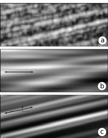
Fig. 2. The effect of slope-aware smoothing. (a) An echogram showing internal sloping layers; (b) smoothing along the horizontal axis; and (c) smoothing along the local layer slope 0 . Direction of smoothing is indicated by the arrows, using x = 15 and σy = 0.5.
The filter spread, a, is chosen x » σy so the filter will primarily smooth along the local layering (Fig. 2c). The smoothed echogram I s can be computed as a convolution between the detrended echogram I and the filter, which can be done efficiently in the frequency domain. The local layer slope Θ for each pixel (x,y) can be found as the θ ∈ {-θmax, ..., θmax} that yielded the strongest response I r to the convolution.
The areas without layer structure will have a random local layer slope with this method (Fig. 3b), and response to the filter I r will be low. To avoid bands of noise in the echograms where no visible layers are present, we filter the echogram vertically using splines assuming that the layer slope is continuous and smooth. Interpolating the slope estimate Θ(x, y) using Ir as weights for the spline yields a smoothed local layer slope 9 c which fills in the interpolated slope for regions without layer structure (Fig. 3c). We set the filter response used as weights to I r = 0 at the bedrock using a coarse pick in order to increase slope estimate accuracy for the near-bedrock layers. If this were not done, the slope of the bedrock would dominate due to the stronger reflection.
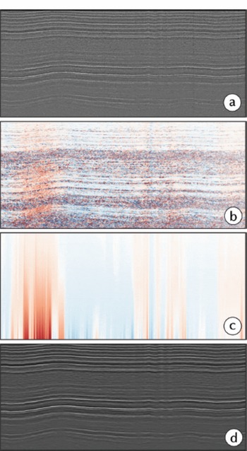
Fig. 3. Estimation of local layer slope. (a) The detrended echogram I; (b) local layer slope 0, with red areas indicating left-to-right ascending layers and blue indicating descending layers; (c) the cleaned local layer slope c ; and (d) the smoothed echogram I s(x,y,Θ c ).
Step 3: seed points to layer estimates
Reference Sime, Hindmarsh and CorrSime and others (2011) showed that integrating the local layer slope can provide first-order approximations to the locations of layers. We set up an interactive user interface for an operator to provide initial seed points on a layer to initialize the integration. For each added point, the initial layer estimate is updated by the distance-weighted average of the mutual integration between pairs of points. The number of operator picks needed depends on the quality of the local layer slope, as small errors in the slope estimation quickly propagate.
Step 4: tracing layers with snakes
An active contour model (Reference Kass, Witkin and WitkinKass and others, 1988) is used to fit the synthetic layer estimates to the echogram. Often referred to as a snake, it consists of a number of knots, interconnected like a string of beads, forming a piecewise linear layer. A snake v with N knots, each described by their location (x, y), can be defined as
Each knot can move within a predefined neighborhood, and the movement is constrained by an internal and external energy function. The energy functions are chosen to have minimal energy when the snake matches an internal layer in the echogram.
The internal energy only depends on the shape of the layer. In the case of fitting internal layers, a desirable internal energy would preserve smooth continuous layering by minimizing the curvature of the snake. The internal energy function E int(v) is chosen to penalize sudden changes in layer slope, where 7 is a scaling parameter and Ф(vi) is the angle formed between the vi - vi _1 and vi +1 - vi edges in the snake.
The external energy only depends on the configuration of the snake relative to the image, or echogram in this case. To cover cases where a layer might briefly disappear, the external energy is chosen to consist of both the mean intensity of the proposed layer E'ext along the snake, and a pattern match E'' ext evaluating how similar the echogram is in the area ψ around the knots, where is the pixel offset from the knot.
Finally, the optimal snake can be found by choosing a v that yields the lowest energy. To balance the energy contributions of each of the terms, a and β are used as scaling parameters.
To simplify the computation, we choose a neighborhood in which the knot can only move vertically, so all possible snakes take the form of a trellis (Fig. 4). If a q-by-p trellis were to be exhaustively searched for the snake that yielded the lowest energy, the computational complexity would be O(qp). This is not feasible to compute. However, with the iterative invocation of the Viterbi dynamic programming algorithm (Reference ForneyForney, 1973; Reference Amini, Weymouth and JainAmini and others, 1990), the computational complexity is reduced to O(mqd), where m « p is the size of the search neighborhood, and d = 3 is the maximum number of knots involved in calculating the energy of a knot.
Fig. 4. One snake (in black) represented on a q-by-p sized trellis where only vertical movement is allowed. The grey nodes represent the neighborhood of possible movement for each knot.
The initial layer estimate is used as the starting configuration of the snake. For each iteration, all permutations of the snake position within the neighborhood are evaluated.
The configuration of the snake that yielded the lowest energy is then used as the starting configuration of the next round of the iteration. If the configuration of the snake was not changed as a result of the iteration, then the lowest energy and optimal snake v optimal has been found.
The scaling parameters a, and are tuned by hand to the specific radar system. First the iterative snake algorithm is run using a = 0, and is tuned to balance the contributions of E'ext and E". In this mode, all smoothness constraints have been disabled and the snake will fit a layer for a while, then jump to a new layer, and so on. If is too small, the snake will not be placed at the intensity peak of the layer in the echogram. With a too large β, the snake will be placed at the global highest intensity in the echogram. Once a balance has been found between the E'ext and E" ext contributions, a can be increased to reduce jumps to adjacent layers. However, if a becomes too large, then the snake will be flat. The 7 parameter can be used to constrain the size of large kinks in the snake.
Results
We processed the sample NGRIP-NEEM transect using the slope estimation and smoothing algorithm previously described (steps 1 and 2). The processing parameters are listed in Table 1. The parameter x is used to control the characteristic length in which the local layer can be considered straight, and θmax is the maximum layer slope we would expect that layer to have. We tuned these parameters by hand, although θmax was chosen to be larger than the steepest layer slope that could be identified from the echogram. The transect was processed using three sets of the parameter pair (θmax,σ x), matching from the steepest to the flattest regions of the internal layers.
Table 1. Parameters used for processing
Ten layers were picked by an operator using an average of 9.8 seed points per layer, with a maximum of 20 for the deepest layer (step 3). The layers were chosen as they were continuous for the entire transect, except for smaller sections of up to ~6 km where the signal was lost. As seen in Figure 5, integrating the local layer slope to form a synthetic layer provides a useful estimate of the actual location of an internal layer. The initial layer estimates were then optimized using the snake-based algorithm (step 4), converging, on average, in 19 iterations. The traced layers are shown in Figure 6. With a coarse spacing of 1.38 km between the knots in the snake, it was not possible to resolve all of the high-frequency undulations in the traced layer.
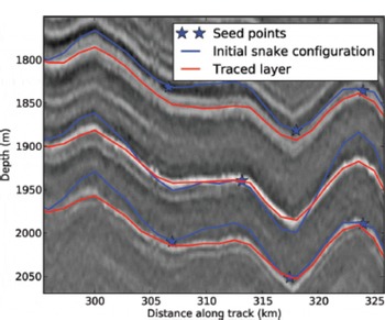
Fig. 5. Tracing layers from seed points. The initial snake configuration (blue lines) from integrating the local layer slope was evolved from the user-picked seed points (blue stars). The layers were traced (red lines) using the initial snake configuration as input to the snake algorithm.
Fig. 6. The full NGRIP–NEEM transect, with the traced layers in red. Ice cores are shown as white vertical lines, with NGRIP to the left and NEEM to the right. The number of picked seed points per layer needed to provide an initial snake configuration averaged 5 for the upper triplet, 9 for the middle four layers and 15 for the lowest triplet.
To evaluate the accuracy of the method, we compared the traced layers to the ice-core age–depth scales. From Figure 7 it is clear that the traced layers are in fact isochrones, as layers match the ice-core chronology within the resolution of the radar.
Fig. 7. Comparison of the traced layers with the ice-core dating. The plot shows the depth difference of the features found at each ice-core site, referenced on the NGRIP depth scale. Black points show the isochronous match points in the two ice cores, and red points show the traced layers at the ice-core sites. Error bars for the red traced layers are based on the resolution of the echogram, ±2 x 2.8 m (one resolution interval per core intersection). This can be compared to the integration of the slope field from NGRIP to NEEM (grey line), which was done without tracing individual layers.
On a standard laptop (2.3 GHz Intel i7 CPU, 16GB memory), the preprocessing of the 423 km transect can be done in <30 min. The manual picking of a seed point takes, on average, 1 min 30 s per layer. Automatically tracing a layer from the manual picks takes <30 s. The automatic layer tracing is not yet optimized for speed, but significant speed increases can be expected, as the algorithm can easily be parallelized.
Discussion
In the formulation of the slope-field-generating algorithm (step 3) we assume that the local layer slope is continuous and smooth. For the interior ice sheet we expect this assumption to be valid; however, in some regions with fast ice flow, discontinuities in the visible layers can appear. Using our method to recover slopes in such regions would lead to incorrectly produced slope fields. We do not recommend using our method in areas where the visible stratigraphy is complex, largely missing or near overturning layers, seen near the bedrock in northern Greenland (NEEM Community Members, 2013). Preliminary applications in regions near the margin suggest that the method is robust to large changes in layer slope. The choice of θmax,σ x and N determines how well layers are traced in such regions. For processing regions with large layer slope, a conservative choice of a large maximum slope angle θ max can be determined directly from the echograms, and should be accompanied by reducing x , the characteristic length in which the layer can be seen approximated as straight. An increased number of snake knots N is also needed to provide a better layer trace, as the traced layer is, by the definition of the snake, piecewise linear between the knots.
Changing the tracing method paradigm from propagation along the track, to tracing the entire layer within two end points, raises new operator challenges. When tracing along track, the algorithm or operator has been required to come up with a metric of when to stop due to the layer quality changing. When tracing the entire layer at the same time, the question is, rather, whether the initial layer estimate for the tracing algorithm is of high enough quality. If the estimate is of bad quality (e.g. crosses multiple layers in the echogram), the snake might get stuck in a local minimum and not trace the intended layer. The quality of the layer estimate can be increased by improvements to the slope field algorithm or by adding additional seed points. Optimizing the layer tracing (step 4) by parallelization has the potential to provide real-time results. Such instant feedback would improve the usability of an interactive layer-tracing tool by an iterative application of steps 3 and 4.
The parameter Ir is a measure of how well the filter matches the layers, and we expect that it can be used as an uncertainty estimate of the slope field. The uncertainty of the slope estimate increases in regions without a clear stratigraphy, which was also reflected by the number of seed points needed to provide an initial layer estimate for the deepest triplet of layers (Fig. 6). Incorporating the slope uncertainty into the snake-tracing energy functions or neighborhood selection can further improve the layer trace.
Conclusion
We have developed two new automated methods for tracing internal layers in radio echograms. The two methods can be used in tandem or applied individually to produce layer slope fields or to optimize existing layer traces. When we apply the methods to trace ten layers over a 423 km transect between two deep ice cores with known age–depth relations, we can verify that the tracing algorithm produces isochrones that match the ice cores within the resolution of the echogram.
The layer-tracing method breaks with the traditional paradigm of propagating layer picks along track by fitting all points of the layer at the same time to the echogram. Automated layer tracing can be done in near-real time from picked seed points, given a preprocessing of the echogram to extract the layer slope. This will allow human operators to be more productive in tracing large-scale datasets.
Acknowledgements
We acknowledge the use of data and data products from CReSIS generated with support from US National Science Foundation grant ANT-0424589 and NASA grant NNX10AT68G. This work was supported by European Research Council Advanced Grant No. 246815 WATERundertheICE.


