


1. Introduction
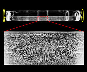
Single-phase flow in a cylindrical container rotating about its axis of symmetry at a constant angular velocity always tends to the solid-body rotation, and therefore axial flow is never sustained. In contrast, multi-phase flow in a rotating cylinder exhibits a surprisingly wide variety of states; see Seiden & Thomas (Reference Seiden and Thomas2011). For example, when we suspend small solid particles in the fluid filled in a container, inertial waves are excited, which lead to a periodic pattern of particle distribution (Lipson Reference Lipson2001; Seiden, Ungarish & Lipson Reference Seiden, Ungarish and Lipson2005). When liquid is partially filled in the cylindrical container, i.e. when there coexist gas and liquid, flow states can be highly non-trivial and the flow is sometimes accompanied with axial flow. It is such non-trivial flow of liquid partially filled in a rotating cylinder (figure 1) that is the target of the present study. Here, we restrict ourselves to the case where the cylinder rotates horizontally about its axis of symmetry.

Figure 1. Schematic of a horizontally rotating cylinder with a liquid–gas interface and the definition of the coordinate system whose origin is set at the centre of the cylinder. We define  $R, L$ and $\boldsymbol {\omega }=(0,0,\omega )$ as the radius, length and angular velocity of the cylinder, and $\boldsymbol {g}=(0, -g, 0)$ as the gravitational acceleration.
Since this flow system is ubiquitous, numerous authors investigated it, in particular, in the regime where a container rapidly rotates. In such a case, fluid forms a film on the wall of the container. This rimming flow is not only scientifically interesting, but also important in engineering applications such as paper manufacturing (Pereira, Valenzuela & Valenzuela Reference Pereira, Valenzuela and Valenzuela2010; Ghosh Reference Ghosh2011; Hubbe Reference Hubbe2021; Majeed et al. Reference Majeed, Pereira, Wang, D'Amico and Kononchek2022), evaporators (Willems et al. Reference Willems, Kroes, Golombok, Van Esch, Van Kemenade and Brouwers2010; Chatterjee, Sugilal & Prabhu Reference Chatterjee, Sugilal and Prabhu2019), centrifugal thermit process (Menekse, Wood & Riley Reference Menekse, Wood and Riley2006), centrifugal casting process (Keerthiprasad et al. Reference Keerthiprasad, Murali, Mukunda and Majumdar2011; Boháček et al. Reference Boháček, Kharicha, Ludwig and Wu2015) and triboelectric nanogenerators (Kim et al. Reference Kim, Chung, Kim, Moon, Lee, Cho, Lee and Lee2016). In fact, flow characteristics such as the instability of the rimming flow were extensively investigated experimentally, theoretically and numerically (Phillips Reference Phillips1960; Yih Reference Yih1960; Johnson Reference Johnson1988; Thoroddsen & Mahadevan Reference Thoroddsen and Mahadevan1997; Hosoi & Mahadevan Reference Hosoi and Mahadevan1999; Tirumkudulu & Acrivos Reference Tirumkudulu and Acrivos2001; Ashmore, Hosoi & Stone Reference Ashmore, Hosoi and Stone2003; Benilov, Benilov & Kopteva Reference Benilov, Benilov and Kopteva2008; Kozlov & Polezhaev Reference Kozlov and Polezhaev2015; Kakimpa, Morvan & Hibberd Reference Kakimpa, Morvan and Hibberd2016; Nicholson et al. Reference Nicholson, Power, Tammisola, Hibberd and Kay2019; Sadeghi, Diosady & Blais Reference Sadeghi, Diosady and Blais2022).
When the rotation of the container is not fast enough to form the rimming flow, a stationary pool of liquid exists at the bottom of the cylinder. We emphasize that flow can be non-trivial even in this regime. More concretely, under some circumstances, flow of partially filled liquid is accompanied by axial motion. The seminal experiments in this flow regime were conducted by Balmer (Reference Balmer1970), who discovered a periodic, in the axial direction, liquid column. Since then, many experimental and theoretical studies revealed patterns of the liquid–gas interface in a rotating cylinder (Benjamin & Pathak Reference Benjamin and Pathak1987; Melo Reference Melo1993; Thoroddsen & Mahadevan Reference Thoroddsen and Mahadevan1997; Thoroddsen & Tan Reference Thoroddsen and Tan2004; Chen et al. Reference Chen, Tsai, Liu and Wu2007). One of the most interesting interface patterns observed in this flow is the shark-teeth-like pattern (Thoroddsen & Mahadevan Reference Thoroddsen and Mahadevan1997). Thoroddsen & Tan (Reference Thoroddsen and Tan2004) visualized flow by using small bubbles as tracers to discover counter-rotating pairs of convection cells, whose axes were perpendicular to the rotation axis of the container. They concluded that the creation of the shark-teeth-shaped interface was relevant to the formation of the convection cells.
We emphasize that the flow sustained in the case with even slower rotations, where the liquid–gas interface is hardly deformed, is still interesting, although only a few authors investigated this regime. The most fascinating phenomenon in this regime is the emergence of the convection cells, whose axis is perpendicular to the rotational axis of the cylinder. Romanò, Hajisharifi & Kuhlmann (Reference Romanò, Hajisharifi and Kuhlmann2017) first numerically demonstrated this phenomenon. Though observed convection cells remind us of those in the experiments by Thoroddsen & Tan (Reference Thoroddsen and Tan2004), we note that the slip boundary condition was imposed on the undeformable liquid–gas interface in the numerical simulations by Romanò et al. (Reference Romanò, Hajisharifi and Kuhlmann2017). They showed that when the Reynolds number  $Re=\omega R^2/\nu$, where $\omega$ is the angular velocity, $R$ is the container radius and $\nu$ is the kinematic viscosity of liquid, satisfied the condition $Re>820\pm 50$, the convection cells could be sustained in the case that the filling ratio, which is defined as the ratio of liquid volume to the container volume, is $\varPsi \approx 0.05$.
Romanò et al. (Reference Romanò, Hajisharifi and Kuhlmann2017) also demonstrated that the convection cells sustained in the pool at the bottom of the container were relevant to liquid mixing. Since counter-rotating pairs of convection cells enhance the stretch and fold of fluid elements, they lead to effective mixing in the liquid phase. This implies that this simple flow system can serve as a bladeless mixer, which is advantageous because we do not need to clean-up blades and because it can avoid damage to delicate materials. This is why many kinds of bladeless mixers were proposed even recently (Goto, Shimizu & Kawahara Reference Goto, Shimizu and Kawahara2014; Meunier Reference Meunier2020; Watanabe & Goto Reference Watanabe and Goto2022; Goto et al. Reference Goto2023). Since the current system is the simplest possible, we expect its wide applications in many fields. Therefore, it is crucial from not only scientific but also engineering viewpoints to reveal the condition that the convection cells are sustained.
Since Romanò et al. (Reference Romanò, Hajisharifi and Kuhlmann2017) showed the critical Reynolds number  $Re_c$ for the onset of the convection cells only for a single condition of the filling ratio, the filling-rate dependence of $Re_c$ is unknown. Furthermore, since their numerical simulation neglects the deformation of the liquid–gas interface, the effect of the deformation on $Re_c$ is also unknown. We also emphasize that although the present system can be categorized in the same group as the Taylor–Couette flow and Rayleigh–Bénard convection, its understanding is poor in contrast to these flows, for which the phase diagram, bifurcations, instability, flow dynamics and so on were extensively examined by many authors. In other words, the present study is one of the first steps to understand this canonical flow.
Thus, the main purpose of this study is to reveal the condition under which the convection cells of partially filled liquid are sustained in the rotating cylinder. As will be described in detail in the following sections, the critical Reynolds number  $Re_c$ depends on the flow conditions such as the filling ratio $\varPsi$ and the Froude number $Fr$ as well as the aspect ratio of the container. In the present study, we determine the critical parameters as accurate as possible and we also develop related arguments on bifurcation structures depending on $\varPsi$. To this end, we conduct both laboratory experiments and direct numerical simulation (DNS). Though experiments are advantageous to discover phenomena, they are sometimes disadvantageous for a systematic parametric survey. This is particularly the case when we consider flow with a liquid–gas interface because it depends both on the Reynolds and Froude numbers; it is impossible to change the former with fixing the latter with the same container and working fluid in experiments. Therefore, we use DNS for the parametric survey. We emphasize that accurate DNS of flow with a free interface is still difficult, although many authors (Keerthiprasad et al. Reference Keerthiprasad, Murali, Mukunda and Majumdar2011; Dawedeit et al. Reference Dawedeit2012; McBride et al. Reference McBride, Humphreys, Croft, Green, Cross and Withey2013; Boháček et al. Reference Boháček, Kharicha, Ludwig and Wu2015; Majeed et al. Reference Majeed, Pereira, Wang, D'Amico and Kononchek2022; Sadeghi et al. Reference Sadeghi, Diosady and Blais2022) already conducted DNS of flow with significant deformations of the liquid–gas interface in the rimming flow. Thus, in the present study, we implement state-of-the-art numerical schemes (Yokoi Reference Yokoi2007; Albadawi et al. Reference Albadawi, Donoghue, Robinson, Murray and Delauré2013; De Vita et al. Reference De Vita, De Lillo, Verzicco and Onorato2021) of multi-phase flow to conduct DNS, which we carefully validate by using experimental data.
2. Method
2.1. Configuration and control parameters
Figure 1 shows the configuration of the examined system, where we drive flow in a cylindrical container with radius  $R$ and axial length $L$ by rotating it at constant angular velocity $\boldsymbol {\omega }$ about its horizontal axis. We partially fill the container with a liquid with density $\rho _l$ and viscosity $\mu _l$. We denote the filling ratio of the liquid by $\varPsi$. We also denote the density and viscosity of gas in the container by $\rho _g$ and $\mu _g$, respectively.
We define Cartesian coordinate  $(x, y, z)$ as shown in figure 1, where the gravitational acceleration $\boldsymbol {g}$ is expressed as $(0,-g,0)$ and the angular velocity $\boldsymbol {\omega }$ of the cylinder as $(0, 0, \omega )$.
Let us summarize the control parameters of the present system. First, the dimensionless length  $L^{*} = L/R$ of the container normalized by $R$ and the filling ratio $\varPsi$ of the liquid are important parameters. Once we fix $L^*$ and $\varPsi$, the flow state depends on the viscous force, inertial force, gravitational force and surface tension. Hence, three control parameters are expressed by the ratios between these forces. Though there are several choices of the three control parameters, we often employ the Reynolds number,
 \begin{equation} Re = \frac{\rho_l R^2 \omega}{\mu_l} , \end{equation}
which is the ratio between the inertial and viscous forces, the Froude number,
 \begin{equation} Fr=\frac{R\omega^2}{g}, \end{equation}
which is the ratio between the inertial and gravitational forces, and the Bond number,
 \begin{equation} Bo=\frac{g\rho_lR^2}{\varPsi\sigma}, \end{equation}
which is the ratio between the gravitational force and the force due to the surface tension. Here,  $\sigma$ denotes the surface tension of liquid. Note that we have adopted the definition of $Bo$ similar to previous studies (Ashmore et al. Reference Ashmore, Hosoi and Stone2003; Sadeghi et al. Reference Sadeghi, Diosady and Blais2022).
In the present study, we restrict ourselves to the cases where the inertial force is much larger than the viscous force; namely,  $Re\gg 1$. However, since the main target is the bifurcation of steady flow, the turbulence regime is beyond the scope of this study. Therefore, we examine the cases with relatively small Reynolds numbers, $Re \lesssim O(10^2)$.
We also restrict ourselves to the cases where the liquid–gas interface is hardly deformed because the gravitational effect dominates the inertial force and surface tension. More concretely, we examine the cases with  $Fr\lesssim 0.1$ for which the inertial force cannot overcome the gravitational force to deform the liquid–gas interface. In all the examined cases, $Bo$ is much larger than $1$ so that we can neglect the effects of surface tension.
Sometimes the flow regimes are classified by the gravitational parameter (Ashmore et al. Reference Ashmore, Hosoi and Stone2003),
 \begin{equation} \varLambda =\frac{\varPsi^2Re}{Fr} , \end{equation}
which denotes the ratio between the gravitational force and the viscous force because it can be rewritten as  $(\rho \delta g)/(\mu ({R\omega }/{\delta }))$, where $\delta (\approx \varPsi R)$ is the thickness of the uniform liquid film for $\varPsi \ll 1$. The flow is classified into three regimes in terms of $\varLambda$ (the shear-dominated regime for $\varLambda \leq 2$, the transitional regime for $2<\varLambda \leq 5$ and the gravitational-dominated regime for $\varLambda > 5$). In the first regime, a coating flow with a nearly uniform liquid film is formed, while the last regime is often called the liquid-pool regime because a stationary pool of liquid is formed at the bottom of the cylinder. Since we examine the cases with small $Fr$, large $Re$ and not so low $\varPsi, \varLambda$ is much larger than $1$. Therefore, according to the classification in terms of $\varLambda$, we deal with the liquid-pool regime.
In summary, the main purpose of the present study is to reveal the conditions of  $L^*, \varPsi$ and $Re$ for the convection cells to appear for sufficiently large $Bo$ (i.e. surface tension is negligible) and sufficiently small $Fr$ (i.e. the liquid–gas interface is hardly deformed). In § 5.3, we will also briefly examine the effect of $Fr$ on flow states.
In experiments, we have to design the set-up so that we can capture the critical Reynolds number  $Re_c$ for the onset of convection cells, which is, as will be shown below, $O(10^2)$. First, as for the size of the experimental apparatus, we use a cylindrical container with radius $R=O(10^{-1})$ m. Then, to satisfy the condition $Bo \gg 1$, we may use either water ( $\sigma = 0.071\ {\rm N}\ {\rm m}^{-1}$) or silicone oil ( $0.0208\ {\rm N}\ {\rm m}^{-1}$) as a working fluid. To satisfy the condition that $Re=O(10^2)$, we must set the angular velocity of the container as $\omega \approx 10^4 \mu _l/\rho _l$. However, if $\omega$ is too small, it is difficult to accurately set the angular velocity with the stepper motor (see figure 2), and tracer particles for visualizations and measurements can settle. Therefore, we use silicone oil, rather than water, with a kinematic viscosity of $\mu _l/\rho _l \approx 50$ cSt so that we can set the angular velocity at $\omega (\approx 1\ \mathrm {rps})$. In this experimental set-up, $Fr$ is $O(10^{-2})$ and therefore the liquid–gas interface is undeformed to keep an almost horizontal flat surface. For DNS, we can set the parameters arbitrarily. For simplicity, however, we ignore the surface tension as well as the wettability in DNS.

Figure 2. (a) Schematic of the experimental apparatus. The acrylic cylindrical container ( $R=50$ mm, $L=800$ mm, thickness 10 mm) rotates about the horizontal axis of symmetry at constant angular velocity $\omega$. The container is partially filled with silicone oil. We observe flow visualized by a laser sheet on the vertical plane. (b) Acrylic jacket to reduce the refraction between the container and air.
When we show results in non-dimensional forms, we use the time and length units of  $\omega ^{-1}$ and $R$, respectively. Non-dimensional time, length and velocity are denoted with superscript $^*$.
$^*$.
2.2. Experimental method
Figure 2(a) shows the schematic of the experimental apparatus. We rotate a cylindrical container with  $R=50$ mm about the horizontal axis. Though we can set containers with different lengths, in the following, we show results with a relatively long cylinder; namely, $L=800$ mm, therefore, $L^*=L/R=16$. The container is made of acrylic with thickness 10 mm. We drive the rotation by a stepper motor (Oriental Motor, ARM66AC-PS10) with the step angle $0.036^\circ$ and a pulse generator (Raspberry Pi 4 model B). The rotation axis precisely coincides with the axis of the cylinder.
As mentioned in the previous subsection, we use silicone oil (Shin-Etsu Silicone, KF96-50cs) as the working fluid. We control the room temperature so that the fluid temperature during experiments is  $25.0\pm 0.3\,^\circ$C. We measure the viscosity of the silicone oil by the viscometer (Kokugo, TVB-10M) and the mass density as 0.0478 Pa s and 955 kg m $^{-3}$, respectively. Therefore, the kinematic viscosity is estimated as $50.1\ {\rm mm}^2\ {\rm s}^{-1}$. Since the surface tension of the silicone oil is $\sigma =0.0208\ {\rm N}\ {\rm m}^{-1}$, the Bond number is $Bo \approx 1.1\times 10^3$ for $\varPsi =1$, which is large enough to neglect the effects of the surface tension. Since we experimentally examine the cases with $\varPsi =0.2$ and 0.4, $0.5{\rm \pi} \ \mathrm {rad}\ \mathrm {s}^{-1} \leq \omega \leq 1.8{\rm \pi} \ \mathrm {rad}\ \mathrm {s}^{-1}, \varLambda$ is always sufficiently large; for example, $\varLambda \approx 69$ for $\varPsi =0.2$ and $\omega =1.8{\rm \pi} \ \mathrm {rad}\ \mathrm {s}^{-1}$.
We seed nylon powder with diameter and density of approximately 50  $\mathrm {\mu }$m and 1.02 $\mathrm {g}\ \mathrm {cm}^{-3}$, respectively, for a volume fraction of approximately 40 ppm and use a continuous laser sheet (Kanomax, CW532-2W, wavelength 532 nm, power 750 mW, width approximately 1.5 mm) on the vertical plane through the horizontal axis to visualize and measure by particle image velocimetry (PIV) the flow on the plane. For the visualization and PIV, we use an acrylic jacket (figure 2b) which is set along the cylindrical container with a clearance of approximately 1 mm. By using this jacket, we can drastically reduce the distortion due to the index mismatch of the acrylic container and air.
The method of flow visualization is as follows. We take images with a digital camera (Nikon, D7100, lens AI Nikkor 20 mm  $f$/2.8S). We use a long exposure time, which is comparable to the spin period of the container, to record the pathlines of flow on the vertical plane. We take, in addition to images of the entire flow, close-up images through the acrylic jacket (figure 2b).
For PIV, we use a digital camera (Ditect, HAS-02M, resolution  $1024 \times 1280$ pixels, frame rate 100 fps) with a lens (Fujinon, DF6HA-1B 6 mm $f$/1.2). To determine the onset of the convection cells in the central region of the cylindrical container, we only record images of the region $128 \times 160$ mm through the jacket (figure 2b). We use the direct correlation method, where we set the interrogation window of size $24\times 24$ pixels to estimate the correlation function. We employ a sub-pixel analysis under the assumption that the correlation function has a normal form. We record the time series of images for 10 revolutions.
Both flow visualizations and PIV are conducted in the steady state after a transient time, approximately 30 revolutions, when we change flow conditions.
2.3. Numerical method
We numerically solve the two-phase Navier–Stokes equation,
 \begin{equation} \rho\left(\frac{\partial \boldsymbol{u}}{\partial t}+\boldsymbol{u} \boldsymbol{\cdot} \boldsymbol{\nabla} \boldsymbol{u}\right)={-}\boldsymbol{\nabla} p+\boldsymbol{\nabla} \boldsymbol{\cdot}(\mu \boldsymbol{D}(\boldsymbol{u}))+\rho \boldsymbol{g} + \rho \boldsymbol{f}, \end{equation}
and the mass conservation equation,
 \begin{equation} \boldsymbol{\nabla} \boldsymbol{\cdot} \boldsymbol{u} = 0,\end{equation}
to simulate flow in the cylinder (figure 1). Here,  $\boldsymbol {u}=(u, v, w)$ is the velocity, $p$ is the pressure and $\boldsymbol {D}(\boldsymbol {u})=\boldsymbol {\nabla } \boldsymbol {u}+(\boldsymbol {\nabla } \boldsymbol {u})^{T}$. Note that the density $\rho$ and viscosity $\mu$ of the fluid (i.e. liquid and gas) are determined by the expression (2.11a,b) explained below. The interaction force $\boldsymbol {f}$ between the fluid and solid is estimated by
 \begin{equation} \boldsymbol{f} = \chi \frac{\boldsymbol{U_f}- \boldsymbol{u}}{\delta t},\end{equation}
where  $\chi$ is the volume fraction of the solid, $\boldsymbol {U_f}$ is the velocity of the solid and $\delta t$ is the numerical time step (Kajishima et al. Reference Kajishima, Takiguchi, Hamasaki and Miyake2001). This method was used, for example, to successfully represent a pipe wall to simulate turbulent flow in it (Ardekani et al. Reference Ardekani, Al Asmar, Picano and Brandt2018). We set the cylindrical shell with wall thickness 12 $\varDelta$, where $\varDelta$ is the numerical grid width in the $x$ direction. Note that we set a uniform orthogonal grid, whose width depends on the direction, in a rectangular computational domain. Then, substituting $\boldsymbol {U_f}=-\omega y \boldsymbol {e}_x+\omega x \boldsymbol {e}_y$ into (2.7), we determine $\boldsymbol {f}$ in the domain. Here, $\boldsymbol {e}_x$ and $\boldsymbol {e}_y$ are the unit vectors in the $x$ and $y$ directions, respectively.
To capture the motion of the liquid–gas interface, we use a simple coupled volume of fluid with the level-set (S-CLSVOF) method (Albadawi et al. Reference Albadawi, Donoghue, Robinson, Murray and Delauré2013), which is a combination of the volume of fluid method (Hirt & Nichols Reference Hirt and Nichols1981) and level-set method (Sussman, Smereka & Osher Reference Sussman, Smereka and Osher1994). Here, we briefly explain this method. First, we solve the advection equation of the volume fraction  $\phi _l$ of liquid,
 \begin{equation} \frac{\partial \phi_{l}}{\partial t}+(\boldsymbol{u} \boldsymbol{\cdot} \boldsymbol{\nabla}) \phi_{l}=0, \end{equation}
by the THINC/WLIC method (Yokoi Reference Yokoi2007). To impose the Neumann boundary condition for  $\phi _l$ on the wall and to set the contact angle as $90^\circ$, we employ the method used in the previous studies (Sussman Reference Sussman2001; Yokoi Reference Yokoi2013; Sun & Sakai Reference Sun and Sakai2016). Second, we set the initial state $\psi _0$ of the level-set function by $0.75(2\phi _l-1)\varDelta$ (Albadawi et al. Reference Albadawi, Donoghue, Robinson, Murray and Delauré2013). We then reinitialize the level-set function $\psi$ by the scheme proposed by Sussman et al. (Reference Sussman, Smereka and Osher1994). In the scheme, we integrate
 \begin{equation} \frac{\partial \psi}{\partial t^{\prime}}= \frac{\psi_{0}}{\sqrt{\psi_{0}^{2}+\varDelta^{2}}}(1- |\boldsymbol{\nabla} \psi|)\end{equation}
to obtain the reconstructed  $\psi$ as the steady solution of (2.9). Here, $t'$ is an artificial time. We conduct this operation at each time step.
We use the level-set function  $\psi$ to define the physical properties of the fluid. The density $\rho$ and viscosity $\mu$ are expressed in terms of a smooth Heaviside function,
 \begin{equation} H(\psi)= \begin{cases}0 & (\psi<{-}\varepsilon), \\ (\psi+\varepsilon) / 2 \varepsilon+\sin ({\rm \pi} \psi / \varepsilon) / 2 {\rm \pi}& (|\psi| \leq \varepsilon), \\ 1 & (\psi>\varepsilon),\end{cases} \end{equation}
where  $\epsilon =1.5\varDelta$. Then, we estimate $\rho$ and $\mu$ by
 \begin{equation} \rho=H(\psi) \rho_{l}+(1-H(\psi)) \rho_{g} \quad \text{and} \quad \mu=H(\psi) \mu_{l}+(1-H(\psi))\mu_{g} ,\end{equation}
respectively.
We use finite difference spatial discretization on the staggered grid. The advection term in (2.5) is expressed by the QUICK method and the other terms are handled by the second-order central difference method. We numerically integrate (2.5) and (2.6) using the SMAC method. For the advection term in (2.5), we use the second-order Adams–Bashforth method, while for the viscous term in (2.5), we use the second-order Crank–Nicolson method modified for two-phase flow (Dodd & Ferrante Reference Dodd and Ferrante2014). We employ the first-order Euler method for the remaining terms. The discretized form of the Poisson equation for pseudo-pressure is solved using the direct method with the fast Fourier transform (Dodd & Ferrante Reference Dodd and Ferrante2014; Frantzis & Grigoriadis Reference Frantzis and Grigoriadis2019; De Vita et al. Reference De Vita, De Lillo, Verzicco and Onorato2021). The Helmholtz equation for the implicit integration of the viscous term is solved iteratively using the SOR method.
In our numerical method, unphysical volume-fraction transfer to the solid region can slightly occur. Since, in some cases, we need more than 100 revolutions of the container to obtain a steady state, we cannot ignore the change in the total volume of the liquid. To overcome this problem, we slightly modify the location of the liquid–gas interface at each time step. First, we integrate the smoothed delta function calculated by
 \begin{equation} \delta_\varepsilon=\left\{\begin{array}{ll} \dfrac{1}{2 \varepsilon}\left[1+\cos \left(\dfrac{{\rm \pi} \psi}{\varepsilon}\right)\right] & |\psi| \leq \varepsilon \\ 0 & |\psi|>\varepsilon \end{array}\right., \end{equation}
to estimate the area  $S$ of the liquid–gas interface. Then, we advect the interface by the pseudo-velocity $\boldsymbol {u}_s=\boldsymbol {\nabla }\psi \delta \phi _l/S\delta t$ to maintain the total volume of the liquid in the container. Here, $\delta \phi _l$ is the difference between the initial and current liquid volumes in the container. In fact, since we deal with the regime where the liquid–gas interface is hardly deformed, the normal direction of the interface $\boldsymbol {\nabla }\psi$ is almost in the $y$ direction. Therefore, we set $\boldsymbol {u}_s \approx (0, \delta \phi _l/S\delta t, 0)$ to the advection velocity of (2.8). We have confirmed that the deviation ratio of the total volume of the liquid in the container is less than 0.01 $\%$ during the numerical integration of flow. Note that we cannot use this method with large deformations of the interface.
For numerical stability, we set the viscosity and density of gas to 1/100 of the liquid. We use the adaptive time step (Frantzis & Grigoriadis Reference Frantzis and Grigoriadis2019) for the integration; namely, we determine  $\delta t$ according to the Courant–Friedrichs–Lewy (CFL) condition. Specifically, we set the time increment $\delta t = Co\varDelta /u_{max}$ at each time step, where $Co$ is the Courant number and $u_{max}$ is the maximum velocity in the computational domain. We set $Co=0.1$ except for the case with $Fr=2.26\times 10^{-3}$ in Run 7 shown in table 2.
3. Experimental results
3.1. Visualization
As mentioned in § 1, convection cells circulating perpendicular to the rotational axis of the container appear in the cylinder. First, we experimentally demonstrate this phenomenon by flow visualizations. We examine two cases with the filling ratio  $\varPsi$ being 0.2 (figure 3) and 0.4 (figure 4), for each of which we change the container's angular velocity $\omega$. Note that $Fr$ changes with $Re$, since we use the same liquid and container in all the cases. In these figures, panels (ai) and (bi) show the entire flow in the container and panels (aii) and (bii) show the flow in a central region of the container which is visualized through the acrylic jacket (figure 2b).

Figure 3. Visualization of pathlines on  $x=0$ plane at $\varPsi =0.2$. The angular velocities are (a) ${\rm \pi}$ and (b) 1.8 ${\rm \pi} \ {\rm rad}\ {\rm s}^{-1}$. We depict (ai and bi) the entire and (aii and bii) a part of the cylindrical container enclosed by the red rectangle in (ai and bi). In (aii and bii), we observe flow through the jacket shown in figure 2(b).

Figure 4. Similar to figure 3, but for  $\varPsi =0.4$. The angular velocities are (a) $0.6{\rm \pi}$ and (b) ${\rm \pi} \ {\rm rad}\ {\rm s}^{-1}$.
We do not observe convection cells in the central region for small  $\omega$ (figures 3a and 4a), while we observe them for larger $\omega$ (figures 3b and 4b). As will be shown by DNS in § 4.3, the convection cells appear through a supercritical pitchfork bifurcation, and the critical angular velocity $\omega _c$ depends on the filling ratio $\varPsi$. In fact, these visualizations (figures 3 and 4) show that $\omega _c$ depends on $\varPsi$. More precisely, $\omega _c$ (and the corresponding Reynold number $Re_c$) for $\varPsi =0.2$ and $0.4$ falls within the ranges ${\rm \pi} \ \mathrm {rad}\ \mathrm {s}^{-1}<\omega _c<1.8{\rm \pi} \ \mathrm {rad}\ \mathrm {s}^{-1} (157< Re_c<282)$ and $0.6{\rm \pi}\ \mathrm {rad}\ \mathrm {s}^{-1}<\omega _c<{\rm \pi}\ \mathrm {rad}\ \mathrm {s}^{-1} (94< Re_c<157)$, respectively.
3.2. PIV
Since we cannot accurately determine  $\omega _c$ (and $Re_c$) only from the visualizations (figures 3 and 4), we quantify the intensity of convection cells using PIV to clarify their onset condition. For this PIV, to avoid the influence of refraction on the air–acrylic-jacket interface and reflection on the liquid–gas interface, we only analyse the bulk of the liquid phase $(-0.8< y^*< h_0^*-0.05)$. Here, $h_0^*$ is the normalized height of the liquid–gas interface without the rotation.
First, we show in figure 5 the mean flow on the  $x=0$ plane, which is obtained by the temporal average over ten revolutions of the container. For $\varPsi =0.2$, we do not observe convection cells at $\omega =1.3{\rm \pi} \ {\rm rad}\ {\rm s}^{-1}$, i.e. $Re=204$ and $Fr=0.085$ (figure 5a), whereas they are visible at $\omega =1.73{\rm \pi} \ {\rm rad}\ {\rm s}^{-1}$, i.e. $Re=272$ and $Fr=0.151$ (figure 5b). For $\varPsi =0.4$, similarly to $\varPsi =0.2$, we observe no convection cells when the angular velocity is smaller ( $\omega =0.7{\rm \pi} \ {\rm rad}\ {\rm s}^{-1}$, i.e. $Re=110$ and $Fr=0.0246$ in figure 5c), while they can be observed at the larger angular velocity ( $\omega =0.8{\rm \pi} \ {\rm rad}\ {\rm s}^{-1}$, i.e. $Re=126$ and $Fr=0.0322$ in figure 5d). To clarify the flow transition, we define an indicator,
 \begin{equation} V^* = max [|v^*(0, y^* ,z_0^*)|],\end{equation}
where  $z_0^*$ is the location of the maximum downward velocity i.e. $z_0^*=0.75$ for $\varPsi =0.2$ and $z_0^*=0$ for $\varPsi =0.4$. We plot $V^*$ as a function of $Re$ in figure 6. We observe that $V^*$ increases significantly above a certain value of $Re$, which is approximately 200 for $\varPsi =0.2$ and approximately 110 for $\varPsi =0.4$. As will be shown by DNS in § 4.3, the convection cells appear through a pitchfork bifurcation. However, the experimental results shown in figure 6 seem different from this bifurcation; namely, the functional form of $V^*$ does not obey $V^* \propto (Re-Re_c)^{1/2}$ for a pitchfork bifurcation (Strogatz Reference Strogatz2018, § 3.4). This is due to two reasons. One is the effect of the end walls. The discussion in § 5.2 will show that the end wall makes the pitchfork bifurcation imperfect, which explains the continuous increase of $V^*$ with $Re$. The other is the fact that $Fr$ changes with $Re$ in the experiments, since we change the angular velocity for the same container and working fluid. In fact, if we take into account the change in $Fr$ (the red crosses in figure 6b), we can explain the functional form of $V^*$; see § 4.1.

Figure 5. Time-averaged velocity fields on  $x=0$ plane. Experimental results with (a) $(\omega, \varPsi )= (1.3{\rm \pi} \ {\rm rad}\ {\rm s}^{-1}, 0.2)$, (b) $(1.73{\rm \pi} \ {\rm rad}\ {\rm s}^{-1}, 0.2)$, (c) $(0.7{\rm \pi} \ {\rm rad}\ {\rm s}^{-1}, 0.4)$ and (d) $(0.8{\rm \pi} \ {\rm rad}\ {\rm s}^{-1}, 0.4)$. The arrows on the frame indicate the wall velocity.

Figure 6. Indicator  $V^*$ defined as (3.1) as a function of $Re$. Experimental results with $L^*=16$ and (a) $\varPsi =0.2$ and (b) $0.4$. Note that $Fr$ changes with $Re$. Red crosses in (b) are the DNS results (see § 4.1) under the same condition as in the experiments (table 1). The vertical lines denote the critical Reynolds number $Re_c$ estimated by DNS (see § 4.3) with slip boundary conditions. The dashed and dotted lines are the results with $Fr=1.81\times 10^{-2}$ and $Fr=9.0\times 10^{-2}$, respectively.
It is worth mentioning the size of convection cells. Flow visualizations in figures 3 and 4 show that the size in the axial direction of the convection cells increases with the filling ratio. This observation is important in practice because the limited length of the cylinder restricts the cell size and affects their onsets. We will discuss this issue in §§ 4.2 and 5.2.
In this section, we have experimentally demonstrated the onset of convection cells. In the next section, we numerically investigate the dependence of the onset on various parameters.
4. DNS results
4.1. Validation
Before the detailed investigation of the onset of convection cells, we validate the numerical method described in § 2.3. To this, we conduct DNS using the same parameters ( $R=0.05$ m, $L=0.8$ m, $\rho _l=955\ \mathrm {kg}\ \mathrm {m}^{-3}, \mu _l=0.0478\ \mathrm {Pa\ s}, \varPsi = 0.4$) as in the experiments shown in § 3. We list the numerical parameters in table 1.
Table 1. Numerical conditions for the validation of DNS:  $\varPsi$, filling ratio; $R$, the radius of the cylinder; $L$, the cylinder length; $\omega$, the magnitude of the angular velocity of the cylinder; $\rho _l$, liquid density; $\mu _l$, liquid viscosity; $g$, the magnitude of the gravitational acceleration; $Co= \delta t \varDelta /u_{max}$, the Courant number; $nx, ny$ and $nz$, the grid numbers in $x, y$ and $z$ directions, respectively. We impose no-slip boundary conditions on the end walls.
First, we visualize the cross-sectional flow on the  $x=0$ plane in figure 7. We can see that DNS results are consistent with the experimental results shown in figure 4. Specifically, no convection cells exist in a central region of the cylinder for $\omega =0.6{\rm \pi} \ {\rm rad}\ {\rm s}^{-1}$, while cells are visible for $\omega ={\rm \pi} \ {\rm rad}\ {\rm s}^{-1}$. We can also confirm that the number of convection cells is 14 in both of the experiment and DNS.

Figure 7. Instantaneous velocity fields on  $x=0$ plane. DNS results, where we impose no-slip boundary conditions on the end walls, with parameters listed in table 1. The angular velocities are (a) 0.5 ${\rm \pi}$, (b) 0.6 ${\rm \pi}$, (c) 0.7 ${\rm \pi}$, (d) 0.8 ${\rm \pi}$, (e) 0.9 ${\rm \pi}$ and (f) ${\rm \pi} \ {\rm rad}\ {\rm s}^{-1}$. The arrows on the frame indicate the wall velocity.
To make a more quantitative comparison, we calculate  $V^*$ defined as (3.1) and plot the results with red crosses in figure 6(b). It is evident that the DNS results are in good agreement with the experimental data. The critical angular velocity, at which $V^*$ starts to increase, also coincides with the experiments.
Here, we mention the treatment of the solid–gas–liquid contact line in DNS. Specifically, the contact angle is set as  $90^\circ$ (see § 2.2), whereas in the experiments, the wall of the container is wet and therefore there is no contact line. The above validation therefore implies that the numerical treatment of the contact line has little effect on the onset of convection cells in the examined regime.
4.2. Dependence of the cell size on  $\varPsi$

As depicted in figures 3 and 4, the axial length  $\lambda ^*$, normalized by $R$, of a pair of convection cells depends on the filling ratio. Here, we numerically investigate the dependence of $\lambda ^*$ on $\varPsi$. For this purpose, we impose slip boundary conditions on the end walls to simulate flow in an infinitely long cylinder. Table 2(a) shows the numerical conditions; we investigate $\lambda ^*$ in the range $0.052 \leq \varPsi \leq 0.9$ under the condition $L^*=64$ and $Fr=1.81\times 10^{-2}$. Here, $\varPsi =0.052$, which corresponds to the case with the liquid height being $0.2R$, is the same filling ratio as in the DNS performed by Romanò et al. (Reference Romanò, Hajisharifi and Kuhlmann2017). To observe the convection cells, we must conduct DNS at a higher Reynolds number than $Re_c$, which depends on $\varPsi$ (see figure 6 for example). This is why we choose $Re$ depending on $\varPsi$ as shown in table 2(a): $Re=200$ for $0.2 \leq \varPsi \leq 0.8, 500$ for 0.1 and 0.9 and 700 for $0.052$. We will discuss the detailed $\varPsi$-dependence of $Re_c$ in the next subsection (see figure 12c).
Table 2. Numerical conditions of DNS to investigate (a) the axial wavelength of the most unstable mode in a sufficiently long cylinder, (b) the critical Reynolds number  $Re_c$ in the cylinder with the length determined by part (a), (c) resolution convergence, (d) the dependence of $Re_c$ on $L^*$, (e) consistency with experiments, (f) the bifurcation at $\varPsi =0.9$ and (g) the dependence of $Re_c$ on $Fr$. We impose slip boundary conditions on the end walls of the cylinder. We list physical and numerical parameters: $\varPsi$, filling ratio; $Re=\rho _lR^2\omega /\mu _l$, the Reynolds number; $Fr=R\omega ^2/g$, the Froude number; $L^*$, the cylinder length normalized by $R$;
$R$;  $Co=\delta t \varDelta /u_{max}$, the Courant number; $nx, ny$ and $nz$, the grid numbers in $x, y$ and $z$ directions, respectively. In the case with $Fr = 2.26\times 10^{-3}$, we set $Co=0.025$ for the sake of numerical stability.
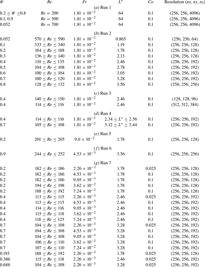
Figure 8 shows the axial velocity component  $w^*$ on the vertical plane ( $x=0$ plane). We observe that the number of convection cells varies with $\varPsi$: that is, 72, 52, 39 and 36 with $\varPsi =0.2, 0.4, 0.7$ and $0.9$, respectively. Thus, we conclude that the length $\lambda ^*$ of a pair of convection cells monotonically increases with $\varPsi$ (figure 9) and the aspect ratio of a convection cell is approximately constant irrespective of $\varPsi$. Incidentally, our result ( $\lambda ^*=0.865$ with $\varPsi =0.052$) is consistent with the result ( $\lambda ^*=0.839 \pm 0.01$) of Romanò et al. (Reference Romanò, Hajisharifi and Kuhlmann2017) with the same $\varPsi$.

Figure 8. Axial velocity component  $w^*$ on $x=0$ plane. DNS (Run 1 in table 2) results under slip boundary conditions on the end walls with (a) $(\varPsi, Re) = (0.2, 200)$, (b) $(0.4, 200)$, (c) ( $0.7, 200$) and (d) ( $0.9, 500$). We set $Fr=1.81\times 10^{-2}$ for all cases.

Figure 9. Wavelength  $\lambda ^*$ obtained by DNS (Run 1 in table 2) under slip boundary conditions on the end walls with cylinder length $L^*=64$ as a function of the filling ratio $\varPsi$. The results with $\varPsi =0.052$ (white circle), 0.1, 0.9 (grey) and 0.2–0.8 (black) are obtained at $Re=700, 500$ and $200$, respectively. We set $Fr=1.81\times 10^{-2}$ for all the cases.
4.3. Dependence of $Re_c$ on $\varPsi$


In this subsection, we examine the filling-rate dependence of  $Re_c$ for the onset of convection cells. Since it requires long computational time to simulate a steady flow in the long cylinder ( $L^*=64$), to reduce them, we conduct DNS of flow in a cylinder with the length $\lambda ^*$ under slip boundary conditions on the end walls. Table 2(b) shows the numerical conditions; as $\lambda ^*$ depends on $\varPsi$ (figure 9), we change the number of grids along the $z$ direction for different $\varPsi$.
First, we visualize flow on the  $x=0$ plane to see its dependence on $Re$ for fixed $\varPsi$ at $0.4$. Figure 10 shows the results for (a) $Re=110$ and (b) $115$ with $\varPsi = 0.4$. The flow has no axial velocity components (figure 10a), while we observe a pair of convection cells at $Re=115$ (figure 10b), implying that $110< Re_c<115$. To clarify the onset of convection cells, we use the indicator (Romanò et al. Reference Romanò, Hajisharifi and Kuhlmann2017)
 \begin{equation} w_r^* = max [{w^*(0, h_0^*-\delta^*, z^*)}],\end{equation}
which quantifies the intensity of convection cells. Here,  $\delta ^*$ denotes a distance from the liquid–gas interface without rotation, and we set $\delta ^* = 0.13$.

Figure 10. Instantaneous velocity fields on  $x=0$ plane. Results of DNS (Run 2 in table 2) under slip boundary conditions on the end walls with $\varPsi =0.4, Fr=1.81\times 10^{-2}$ and (a) $Re=110$ and (b) $115$. The cylinder length is set as $L^*=\lambda ^*=2.46$. The arrows on the frame indicate the wall velocity.
We plot the temporally averaged value  $\overline {w^*_r}$ as a function of $Re$ for $\varPsi =0.4$ and 0.7 in figure 11(a). For $\varPsi =0.4, \overline {w^*_r}$ vanishes at $Re=110$, and $\overline {w^*_r}$ starts to increase at $Re \approx 114$ as $Re$ increases. This observation implies that the convection cells appear through a supercritical bifurcation. For $\varPsi =0.7, \overline {w^*_r}$ starts to increase at $Re \approx 108$, which is smaller than the value for $\varPsi =0.4$. To determine $Re_c$ precisely, we use the feature that if the convection cells appear through a pitchfork bifurcation, $\overline {w^*_r}$ follows
 \begin{equation} \overline{w^*_r}=c\sqrt{Re-Re_c},\end{equation}
where  $c$ is a constant. We determine $Re_c$ by fitting three values of $\overline {w^*_r}$ in the range of $Re$ above and nearest $Re_c$. Dashed lines in figure 11(a) show the fitting curves. Thus, determined critical Reynolds numbers for $\varPsi =0.4$ and 0.7 are $112.9$ and $106.4$, respectively.

Figure 11. (a) Time-averaged intensity  $\overline {w^*_r}$ of convection cells defined as (4.1) as a function of $Re$ for two different values of the filling ratio: $\circ, \varPsi =0.4$; $\bullet, 0.7$. The cylinder length $L^*$ is set as $\lambda ^*$ shown in figure 9. Dashed lines represent the fitting by (4.2). Results of DNS (Run 2 in table 2) under slip boundary conditions on the end walls. (b) Relationship between $Re_c$ and $\alpha (=L^*/\lambda ^*)$. The symbols are the same as in (a). Dashed lines represent the quadratic function passing three points of ( $\alpha, Re_c$). Results of DNS (Run 3 in table 2) under slip boundary conditions on the end walls.
Here, we briefly mention the mesh convergence. We conduct DNS (table 2c) with three different grid numbers:  ${DNS_{coarse}} [(nx, ny, nz) = (128, 128, 96)]$, ${DNS_{medium}} [(nx, ny, nz) = (256, 256, 192)]$ and ${DNS_{fine}} [(nx, ny, nz) = (512, 512, 384)]$. Table 3 shows $Re_c$ for the three cases together with $Re$ and $\overline {w^*_r}$, which are used to determine $Re_c$. Although the value of $Re_c$ obtained by ${DNS_{coarse}}$ differs significantly from that by ${DNS_{medium}}, Re_c$ obtained by ${DNS_{fine}}$ matches the result of ${DNS_{medium}}$ with only $1\,\%$ relative difference. Therefore, we conclude that ${DNS_{medium}}$ is fine enough to estimate $Re_c$.
Table 3. Dependence of the critical Reynolds number  $Re_c$ on the numerical resolution under the condition $\varPsi =0.4, Fr=1.81\times 10^{-2}$ and $L^*= \lambda ^*$. We also show the data for fitting by (4.2). For the fitting, we use three values of $\overline {w^*_r}$ at $Re=Re_1, Re_2$ and $Re_3$.

Next, we briefly mention the dependence of  $Re_c$ on the cylinder length $L^*$. Recall that, in Run 2 (figure 11a), we set $L^*$ as the axial wavelength $\lambda ^*$ of the cells sustained in a long cylinder ( $L^*=64$). Recall also that we impose slip boundary conditions on the end walls in Run 2 to mimic an infinitely long cylinder. To examine the effects of $L^*$ on $Re_c$, we set $L^*$ as
 \begin{equation} L^{*}=\alpha \lambda^*,\end{equation}
where  $\alpha$ is a positive coefficient; see table 2(d) for the numerical conditions. Figure 11(b) shows $Re_c$ as a function of $\alpha$ for $\varPsi =0.4$ and $0.7$. We can see that $Re_c$ takes the minimum at approximately $\alpha = 1$ in both cases. This result implies that $\lambda ^*$ approximates the wavelength of the most unstable mode in the infinite-length cylinder.
To investigate the  $\varPsi$ dependence of $Re_c$, we apply the above method for various values of $\varPsi$. Figures 12(a) and 12(b) show $\overline {w^*_r}$ as a function of $Re$. Since $\overline {w^*_r}$ is well fitted by (4.2), we may conclude that the convection cells appear through a pitchfork bifurcation for $0.052 \leq \varPsi \leq 0.8$. We also plot $Re_c$ as a function of $\varPsi$ in figure 12(c). We can see that $Re_c$ depends on $\varPsi$ non-monotonically and it takes minimum at $Re_c \approx 100$ around $0.5 \lesssim \varPsi \lesssim 0.7$. Incidentally, we do not show the result for $\varPsi =0.9$ in figure 12(a) because, as will be shown in detail in § 5.1, the convection cells appear through a subcritical bifurcation for $\varPsi =0.9$.

Figure 12. (a) Time-averaged intensity  $\overline {w^*_r}$ of convection cells defined as (4.1) as a function of $Re$. Different symbols denote results with different values of the filling ratio: $\lozenge$, $\varPsi =0.052$; $\triangleleft$, $0.1$; $\square, 0.2$; $\triangleright$, $0.3$; $\circ, 0.4$; $\triangledown$, $0.5$; $\triangle, 0.6$; $\bullet, 0.7$; $\times, 0.8$. Dashed lines represent the fitting by (4.2). (b) Same as (a) but for the close-up view in the range $90 \leq Re \leq 150$. (c) $Re_c$ as a function of $\varPsi$. Results of DNS (Run 2 in table 2) under slip boundary conditions on the end walls.
To compare the obtained  $Re_c$ with experimental results, we plot vertical dashed lines at $Re_c$ in figures 6(a) and 6(b). For $\varPsi =0.4$, the dashed line well explains the experimental observation that $V^*$ starts to increase as $Re$ increases above a value around $Re_c$. However, for $\varPsi =0.2$, we see the discrepancy between $Re_c$ and the Reynolds number above which $V^*$ increases. This discrepancy is mainly caused by the difference in $Fr$. In DNS, we fix $Fr$ to determine $Re_c$. In contrast, $Fr$ changes with $Re$ in the experiments. Figure 6(a) shows that the cells in the experiments appear at $Re \approx 200$ for $\varPsi =0.2$. In this condition, $Fr$ is $9.0\times 10^{-2}$, which differs significantly from the value ( $1.81\times 10^{-2}$) in DNS. Therefore, to confirm the consistency between the experiments and DNS, we estimate $Re_c$ with $Fr = 9.0\times 10^{-2}$ for $\varPsi =0.2$ by DNS (table 2e). The result ( $Re_c \approx 200$) is shown by the vertical grey dotted line in figure 6(a), which well explains the experiments (figure 6a). Incidentally, for $\varPsi =0.4$, the convection cells appear at $Re \approx 110$ (figure 6b), and in this experimental condition, $Fr \approx 2.6\times 10^{-2}$. In fact, the difference in $Fr$ between DNS and the experiment has little influence on $Re_c$ in this small- $Fr$ range (see figure 18a in § 5.3).
It is worth comparing our results with the previous study (Romanò et al. Reference Romanò, Hajisharifi and Kuhlmann2017). They showed that the critical Reynolds number was approximately 820 for  $\varPsi =0.052$. This is significantly larger than the value ( $Re_c=562$) in our DNS. Although their DNS does not account for interface deformation, it seems not the main cause. To confirm this, we have conducted DNS with sufficiently small $Fr$ ( $=4.53\times 10^{-3}$); even if we set $L^*$ as done by Romanò et al. (Reference Romanò, Hajisharifi and Kuhlmann2017), the obtained value of the critical $Re$ is approximately 560, which is almost the same as the value (562) for the larger $Fr$ ( $1.81\times 10^{-2}$). In addition, we have also conducted experiments with the filling ratio as used by Romanò et al. (Reference Romanò, Hajisharifi and Kuhlmann2017), the results (see Appendix A) support the value of $Re_c$ obtained by the present DNS.
5. Discussion
In this section, we investigate three issues. First, we investigate the onset of convection cells for  $\varPsi \rightarrow 1$. As described in § 4.3, convection cells appear through a pitchfork bifurcation for $0.052 \leq \varPsi \leq 0.8$. In contrast, when $\varPsi =1$, the solid-body rotational flow is always stable for any $Re$. Since the connection of these two regimes is unclear, we investigate flow bifurcation at $\varPsi =0.9$. Second, we investigate the effect of the end walls of the cylindrical container on the flow. Since real containers have end walls, it is important to investigate their effect on the bifurcation. Third, we examine the dependence of $Re_c$ on $Fr$.
$Fr$.
5.1. Onset of convection cells at $\varPsi =0.9$

In the previous section, we have demonstrated that convection cells appeared through a supercritical pitchfork bifurcation for  $0.052 \leq \varPsi \leq 0.8$. However, regardless of $Re$, we cannot observe convection cells when the container is filled with liquid (i.e. $\varPsi =1$). This means that the simple two-dimensional rotating flow is linearly unstable for $Re>Re_c(\varPsi )$ in the examined range of $\varPsi$ ( $\leq 0.8$), whereas it is always stable at $\varPsi =1$. To understand how these two regimes are connected, here we investigate the onset of convection cells and its bifurcation structure at $\varPsi =0.9$.
Table 2(f) shows the numerical conditions, where we set the Froude number as  $Fr=4.53\times 10^{-3}$. This value is smaller than in DNS shown in the previous section, so that we can further reduce the effect of the oscillation of the liquid–gas interface on the flow. As will be described in § 5.3, this Froude number is sufficiently small to neglect the dependence of $Fr$ on the flow.
We show the bifurcation diagram by using  $\overline {w^*_r}$, which is defined as (4.1), in figure 13(a). We can see that the diagram differs from those in the cases with $0.052 \leq \varPsi \leq 0.8$ (figures 11a and 12a). We have drawn this diagram (figure 13a) through the following procedure. First, we simulate the steady state with convection cells at $Re=252$, then gradually decrease $Re$ to plot filled circles. Although the intensity $\overline {w^*_r}$ of convection cells decreases as $Re$ decreases, they still exist for $Re \gtrsim 245$. However, $\overline {w^*_r}$ suddenly drops to zero at $Re=244$, indicating the disappearance of convection cells. However, when increasing $Re$ from the flow state without convection cells at $Re=244, \overline {w^*_r}$ remains at 0 (open squares in figure 13a) in a range of $Re$, but $\overline {w^*_r}$ suddenly increases and reaches the value (the filled circle) obtained by decreasing $Re$ when the Reynolds number reaches $Re=248$. This dependence of $\overline {w^*_r}$ on $Re$ implies that the convection cells appear through a subcritical bifurcation at $\varPsi =0.9$ for sufficiently small $Fr$. It is worth looking at the differences in the convection cells that appear through supercritical and subcritical bifurcations. We compare the two cases in figure 14. Although the velocity fields shown in figures 14(a) and 14(b) appear through supercritical and subcritical bifurcations, respectively, we can observe no quantitative difference in the flow.

Figure 13. (a) Time-averaged intensity  $\overline {w^*_r}$ of convection cells defined as (4.1) as a function of $Re$. Black-filled circles and open squares are obtained when $Re$ decreases and increases, respectively. Open circles represent the unstable solutions. (b) Temporal evolution of the intensity $w_r^*$ of the convection cells at $Re=245$ with various initial conditions. Solid and dashed lines indicate the increasing and decreasing functions of time, respectively. (c) Time derivative $k$ of $w_r^*$ in (b) as a function of the time-averaged intensity $\overline {w_r^*}'$ of convection cells for $20{\rm \pi} \leq t^* \leq 40{\rm \pi}$. Results of DNS (Run 6 in table 2) with $\varPsi =0.9$ and $L^*=\lambda ^*$ under slip boundary conditions on the end walls.

Figure 14. Instantaneous velocity fields just above the onset of the convection cells via (a) supercritical and (b) subcritical bifurcations. We show velocity fields on (i)  $x^*$ = $0$, (ii) $-0.25$ and (iii) $0.25$ planes for (a) $(\varPsi, Re)=(0.4, 118)$ and (b) $(0.9, 246)$. DNS (Run 6 and 7 for (b) and (a), respectively, in table 2) results with $Fr=4.53\times 10^{-3}$ and $L^*=\lambda ^*$ under slip boundary conditions on the end walls.
As the convection cells appear through a subcritical bifurcation in the case with  $\varPsi =0.9$, there are unstable solutions between the upper and lower branches in figure 13(a). To confirm this, we obtain them using a simpler procedure than the conventional ones such as the shooting method.
Here, we explain the method to obtain the unstable solutions at  $Re=245$, for example. First, we construct four initial conditions which have different intensities of convection cells. To obtain them, we simulate flow at $Re=244$ with the initial condition of the steady state at $Re=250$. As shown in figure 13(a), since the convection cells cannot be sustained at $Re=244$, they monotonically decay. Then, we select flow fields at four instances in this decaying process as initial conditions for the runs at $Re=245$. We plot in figure 13(b) the evolution of the intensity $w_r^*$ at $Re=245$ with the four initial conditions. For the initial conditions with $w_r^*>0.07, w_r^*$ increases with time, whereas for those with $w_r^*<0.07, w_r^*$ decreases. Since $w_r^{*}$ does not increase or decrease on the unstable branch, we can estimate an unstable solution by identifying the point at which the time derivative $k$ of $w_r^*$ becomes zero. We evaluate $k$ by least-square fitting of $w_r^*(t^*)$ between $t^*=20{\rm \pi}$ and $40{\rm \pi}$. Figure 13(c) shows $k$ as a function of $\overline {w_r^*}=({1}/{20{\rm \pi} }) \int ^{20{\rm \pi} }_{40{\rm \pi} }{w_r^{*}(t^*)}\,\mathrm {d}t^*$. The value of $k$ increases monotonically with $\overline {w_r^*}'$, and $k \approx 0$ at $\overline {w_r^*}'\approx 0.069$. We estimate $\overline {w_r^*}'$ for $k=0$ by the linear interpolation between two data points at approximately $k=0$. We plot $\overline {w_r^*}'$ for $k=0$, corresponding to unstable solutions in the range $244.7\leq Re \leq 247.5$ in figure 13(a) with open circles. Thus, from figure 13(a), we conclude that convection cells appear through a subcritical bifurcation at $\varPsi =0.9$.
We have shown the overall bifurcation structures (i.e. the supercritical pitchfork bifurcation for  $\varPsi \leq$ 0.8 and the subcritical bifurcation at $\varPsi =0.9$) of the present system. To obtain a more detailed understanding of the bifurcation, in particular, in the range $0.8<\varPsi <0.9$, further investigation by linear stability analysis is required, which we leave for a future study. Incidentally, we do not experimentally observe the subcritical bifurcation for $\varPsi =0.9$ due to the effect of the end walls.
5.2. The effect of end walls on the convection cells
In § 4, we investigate flow in the cylinder under the slip boundary conditions on the end walls. This was intended to simulate flow in an infinitely long cylinder. However, since the cylinder's length is finite in practice, we investigate, in this subsection, the influence of the end walls on the onset of the convection cells by imposing no-slip boundary conditions on the walls.
Table 4(a) shows numerical conditions for this purpose. We examine the onset of convection cells in a finite-length cylinder with two different values of the filling ratio:  $\varPsi =0.4$ and 0.7. First, we investigate the dependence of flow on the cylinder length $L^*$ and the Reynolds number $Re$. More concretely, in each case of the filling ratios, we set $L^*$ as $\alpha \lambda ^*$ with $\alpha$ being $1, 2$ and $3$, where $\lambda ^*$ is the normalized wavenumber corresponding to the most unstable mode in the infinitely long cylinder.
Table 4. Numerical conditions of DNS to investigate effects of (a) the end walls and (b) the cylinder length on the onset of convection cells. We set no-slip boundary conditions on the end walls.

We define the indicator as
 \begin{equation} E_{{axis}}=\overline{\langle w^{*2} \rangle},\end{equation}
of the axial flow intensity to quantify the effects of  $L^*$ and $Re$ on the flow. Here, $\langle {\cdot } \rangle$ denotes the volume average weighted by $\phi _l$. We plot $E_{{axis}}$ as a function of $Re$ for $\varPsi =0.4$ and $0.7$ in figures 15(a) and 15(b), respectively. In both cases of $\varPsi$, we observe, irrespective of $\alpha$, that $E_{{axis}}$ increases monotonically with $Re$. We can also notice that the dependence of $E_{{axis}}$ on $Re$ approaches the case under slip boundary condition (§ 4.3) as $\alpha$ increases. This tendency is independent of $\varPsi$ and implies that the presence of the no-slip end walls makes the pitchfork bifurcation imperfect. In fact, the imperfect pitchfork bifurcation approaches the perfect one as $L^*$ increases because the influence of end walls becomes smaller. Note that we consider the cases with integer $\alpha$. If $\alpha$ is a non-integer, the dependence of the $E_{{axis}}$– $Re$ curve approaches non-monotonically to the dashed line as $\alpha$ increases. It might be worth comparing the present results with those for cavity flow because Blohm & Kuhlmann (Reference Blohm and Kuhlmann2002) experimentally showed that convection cells in a two-sided lid-driven cavity also appeared through an imperfect pitchfork bifurcation.

Figure 15. Indicator  $E_{{axis}}$ defined as (5.1) of the magnitude of the axial velocity as a function of $Re$ at $Fr=1.81\times 10^{-2}$. The filling ratios are (a) $\varPsi =0.4$ and (b) $0.7$. Different symbols denote results for different cylinder lengths: white, $\alpha =1$; grey, $2$; black, $3$. Dashed lines denote the result for $\alpha =1$ but with slip boundary conditions on the end walls. Results of DNS Run 8, where we impose no-slip boundary conditions on the end walls, in table 4.
Next, we investigate the influence of  $L^*$ on the flow at fixed Reynolds number ( $Re=200$) and Froude number ( $Fr=1.81\times 10^{-2}$); the other numerical conditions are listed in table 4(b). Recall that under this condition, convection cells appear because $Re>Re_c$ for $\varPsi =0.4$ and $0.7$ and $Fr=1.81\times 10^{-2}$ (see figure 12c). First, we visualize flow in figure 16 for $\varPsi =0.7$ on the $x=0$ plane to demonstrate the dependence of flow on $L^*$. We observe that the flow strongly depends on $\alpha$. When $\alpha$ is an integer (figure 16b,d,e), we observe convection cells, and the number of pairs of cells is equal to $\alpha$. In contrast, when $\alpha =0.7$ and $1.5$, we do not observe any cells. This observation implies that the cylinder length significantly affects the intensity of convection cells. To more qualitatively understand the dependence of the intensity of convection cells on the cylinder length, we plot $E_{{axis}}$ as a function of $\alpha$ in figure 17 for $\varPsi =0.4$ and $0.7$. In both cases of $\varPsi, E_{{axis}}$ exhibits non-monotonic dependence on $\alpha$, and $E_{{axis}}$ has local maxima when $\alpha$ is close to an integer. This observation implies that the length $L^*$ of the container is appropriate when it is an integer multiple of $\lambda ^*$ to sustain the convection cells. It also implies that the optimal length is independent of the boundary condition on the end walls. Recall that results in figure 17 are obtained under no-slip boundary conditions, whereas those in figure 11 are under the slip boundary conditions.

Figure 16. Instantaneous velocity fields on  $x=0$ plane with various cylinder lengths $L^*=\alpha \lambda ^*$ at $Re=200$ under the condition $\varPsi =0.7$ and $Fr=1.81\times 10^{-2}$. We impose no-slip boundary conditions on the end walls. Results of DNS (Run 9 in table 4) for (a) $\alpha = 0.7$, (b) $1$, (c) $1.5$, (d) $2$ and (e) $3$. The arrows on the frame indicate the wall velocity.

Figure 17. Indicator  $E_{{axis}}$ defined as (5.1) of the magnitude of the axial velocity as a function of $\alpha (=L^*/\lambda ^*)$ with $Fr=1.81\times 10^{-2}$ and $Re=200$. The symbols are the same as in figure 11(a). Results of DNS (Run 9 in table 4) under no-slip boundary conditions on the end walls.
The results obtained in this subsection may be valuable for designing mixers that use these convection cells. For rapid mixing, we should select  $L^*$ as an integer multiple of $\lambda ^*$. For instance, Varley, Markaki & Brooks (Reference Varley, Markaki and Brooks2017) conducted experiments to investigate the relationship between liquid flow in a partially filled cylindrical container and cell culture efficiency. Although they did not observe convection cells probably because of the unoptimized cylinder length, their conclusions might differ if they used a cylinder with different $L^*$. Since we can generate desirable flow by appropriately setting the cylinder length, filling ratio and angular velocity, this system has potential for mixing devices in various applications. In particular, this system may be useful in bioengineering such as cell culture, which requires precise control of flow.
5.3. Dependence of $Re_c$ on $Fr$


In § 4, we have discussed  $Re_c$ for a single value of $Fr$ (i.e. $1.81\times 10^{-2}$). In this subsection, we investigate the dependence of $Re_c$ on $Fr$. Since the objective of the present study is to clarify the onset of convection cells in the liquid-pool regime, we investigate the $Fr$ dependence of $Re_c$ in a small- $Fr$ range, $2.26\times 10^{-3} (= Fr_0)\leq Fr \leq 7.24\times 10^{-2} (= Fr_1)$ for each of three filling ratios, $\varPsi =0.2, 0.4$ and $0.7$ (table 2g).
Using the method described in § 4.3, we identify  $Re_c$ for each combination of $Fr$ and $\varPsi$ to clarify the relative increase,
 \begin{equation} \Delta Re_c(Fr, \varPsi; Fr_0, \varPsi) = \frac{Re_c(Fr, \varPsi)-Re_c(Fr_0,\varPsi)}{Re_c(Fr_0,\varPsi)},\end{equation}
from the value at the reference Froude number  $Fr_0$. Figure 18(a) shows $\Delta Re_c$ as a function of $Fr$ for $\varPsi =0.2, 0.4$ and $0.7$. We observe that as $Fr$ increases, $\Delta Re_c$ increases for all the examined $\varPsi$, though $\Delta Re_c$ is negligibly small for $Fr \lesssim 4 \times 10^{-3}$. This implies that the flow does not significantly depend on $Fr$ in the small- $Fr$ range. We also observe that $\Delta Re_c$ in a large- $Fr$ range is larger for smaller $\varPsi$.

Figure 18. (a) Relative difference  $\Delta Re_c$ defined as (5.2) of $Re_c$ as a function of $Fr$. (b) Variation of liquid height $\Delta h^*$ defined as (5.3) at the centre of the cylinder as a function of $Fr$. (c) Magnitude of circulation velocity $U_s$ defined as the second equation in (5.4) as a function of $Fr$. The symbols in panels (a), (b) and (c) are the same as in figure 12(a). (d) Relative differences of the critical Reynolds number at $Fr=2.26\times 10^{-3}$ and $7.24\times 10^{-2}$. Different colours of charts denote the result with different definitions of the relative differences: white, the relative difference defined as (5.2); black, both $Re^e$ and $\varPsi ^e$ are considered; light grey, only $Re^e$ is considered; dark grey, only $\varPsi ^e$ is considered. These results are obtained by DNS (Run 7 in table 2) with $L^*=\lambda ^*$ under slip boundary conditions on the end walls.
We now explain the observed  $Fr$ dependence of $Re_c$ by introducing the effective filling ratio $\varPsi ^{e}$ and the effective Reynolds number $Re^{e}$.
First, we examine the dependence of  $\varPsi ^{e}$ on $Fr$. Here, we define $\varPsi ^{e}$ by using the liquid height at the centre of the cylinder. Since the container's motion lifts the liquid more easily for larger $Fr$, the liquid height in a central region decreases for large $Fr$. To qualify this change, we define
 \begin{equation} \Delta h^* = \overline{h^*-h_0^*},\end{equation}
where  $h^*$ is the $y^*$-coordinate satisfying $\phi _l(0,y^*,0)=0.5$. We examine flow at $Re$ slightly lower than $Re_c$ to discuss the $Fr$ dependence of $Re_c$ on $Fr$. Since the flow at $Re (< Re_c)$ is two-dimensional, we conduct two-dimensional simulations to estimate $\Delta h^*$. Figure 18(b) shows the estimated variation $\Delta h^*$ as a function of $Fr$. We can see that $\Delta h^*$ and therefore $\varPsi ^e$ decrease monotonically as $Fr$ increases. We emphasize that $\varPsi ^{e}$ differs depending on $Fr$ even if $\varPsi$ is the same.
Second, we examine the  $Fr$ dependence of $Re^{e}$, which we define as
 \begin{equation} Re^e = \rho_l U_sR/ \mu_l \quad \text{with } U_s = \langle u^2+v^2\rangle^{1/2}. \end{equation}
It is known that the deformation of the interface affects the circulation velocity in the liquid phase (Terrington, Hourigan & Thompson Reference Terrington, Hourigan and Thompson2020). Hence,  $Re^e$ depends on $Fr$ because of interface deformations for large $Fr$. Figure 18(c) shows $U_s$, which is estimated by the two-dimensional simulations, as a function of $Fr$. We can see that $U_s$, and therefore $Re^e$, depend on $Fr$ at any $\varPsi$. Therefore, $Re^{e}$ differs for the different value of $Fr$ even if $Re$ is the same.
We are ready to explain the  $Fr$ dependence of $Re_c$ by using $Re^e$ and $\varPsi ^e$. More concretely, we show that $\varPsi ^e$ determines $Re_c^e$ even when $Fr$ is significantly different. To show this, we need to set two conditions where $\varPsi ^e$ is common, but $Fr$ is significantly different. However, since we cannot prescribe $\varPsi ^{e}$, we use the numerical observation that $\varPsi ^{e}$ is almost the same as $\varPsi$ for sufficiently small $Fr$ (figure 18b). Figure 19 shows the construction of the two sets of parameters such that $Fr$ is significantly different but $\varPsi ^e$ is almost common. The first set of parameters is $Fr=Fr_1$ and $\varPsi$ (figure 19a). Under this condition, we conduct DNS to obtain $\varPsi ^e(Fr_1, \varPsi ), Re_c(Fr_1, \varPsi )$ and $Re_c^e(Fr_1, \varPsi )$. Note that $\varPsi \gg \varPsi ^e(Fr_1, \varPsi )$ because $Fr_1$ is sufficiently large (figure 19a). The second set is $Fr=Fr_0$ and $\varPsi =\varPsi ^e(Fr_1, \varPsi )$ (figure 19b). Since $Fr_0$ is sufficiently small, $\varPsi ^e(Fr_0) \approx \varPsi ^e(Fr_1)$. Then, we obtain, by DNS, $Re_c(Fr_0, \varPsi ^e(Fr_1, \varPsi ))$ and $Re^e_c(Fr_0, \varPsi ^e(Fr_1, \varPsi ))$. Thus, we can obtain the critical Reynolds numbers, $Re_c$ and $Re_c^e$, at two different parameter sets ( $Fr_1, \varPsi$) and ( $Fr_0, \varPsi ^e(Fr_1, \varPsi )$). Note that $\varPsi \gg \varPsi ^e(Fr_1, \varPsi )$ and $Fr_1 \gg Fr_0$, but $\varPsi ^e$ is almost common for these two parameter sets.

Figure 19. Schematics of the liquid–gas interface with two sets of parameters (a)  $(Fr, \varPsi ) = (Fr_1, \varPsi )$ and (b) $(Fr_0, \varPsi ^e(Fr_1, \varPsi ))$ such that $Fr$ is significantly different but $\varPsi ^e$ is almost common. Solid circles indicate the cylindrical walls. Solid and dashed lines represent the liquid–gas interfaces with and without rotation, respectively. Since $Fr_1$ is sufficiently large, $\varPsi \gg \varPsi ^e(Fr_1, \varPsi )$, whereas since $Fr_0$ is sufficiently small, $\varPsi \approx \varPsi ^e(Fr_1, \varPsi )$. Arrows represent the liquid height at the centre of the cylinder with a rotation, whose lengths in (a) and (b) are almost the same.
We confirm our hypothesis that  $Re^e_c$ is determined by $\varPsi ^e$ in three cases of $\varPsi$: $0.2, 0.4$ and $0.7$. To this, we define
 \begin{equation} \Delta Re^{e}_c(Fr_1, \varPsi; Fr_0, \varPsi_0) = \frac{Re^{e}_c(Fr_1, \varPsi)-Re^e_c(Fr_0, \varPsi_0)}{Re^e_c(Fr_0, \varPsi_0)}.\end{equation}
White charts in figure 18(d) show  $\Delta Re_c(Fr_1, \varPsi ; Fr_0, \varPsi )$ and black ones show $\Delta Re_c^e(Fr_1, \varPsi ; Fr_0, \varPsi ^e(Fr_1, \varPsi ))$. It is notable that the latter is significantly smaller than the former for all the three cases of $\varPsi$. This means that the dependence of $Re_c$ on $Fr$ is explained by $\varPsi ^e$ and $Re^e$.
We emphasize that it is crucial to consider both of  $Re^e$ and $\varPsi ^e$. To demonstrate this, we show the relative differences when considering only $Re^e$ (i.e. $\Delta Re^{e}_c(Fr_1, \varPsi ; Fr_0, \varPsi )$) or $\varPsi ^e$ (i.e. $\Delta Re_c(Fr_1, \varPsi ; Fr_0, \varPsi ^{e}(Fr_1, \varPsi )$) in figure 18(d). It is evident that these are larger than $\Delta Re_c^e(Fr_1, \varPsi ; Fr_0, \varPsi ^e(Fr_1, \varPsi ))$. Furthermore, in the case of $\varPsi =0.7$, the relative difference when considering only $\varPsi ^e$ exceeds the original one. These results conclude the necessity of considering both $Re^e$ and $\varPsi ^e$ to understand the dependence of $Re_c$ on $Fr$.
$Fr$.
6. Conclusions
Convection cells can be sustained in liquid phase in a constantly rotating cylinder which is partially filled with liquid (figure 1). We have investigated this canonical flow phenomenon in detail by experiments and DNS.
First, we have demonstrated the onset of convection cells by experiments using a long ( $L^* = L/R =16$) cylindrical container (figure 2). When the angular velocity is small enough, we do not observe the convection cells, but they are visible for a larger angular velocity (figures 3 and 4). To identify the onset of the convection cells, we have quantified the intensity of convection cells by using the data obtained by PIV (figure 5) as a function of $Re$ (figure 6). We can observe flow transition around a certain Reynolds number $Re_c$, which depends on the filling ratio $\varPsi$. To systematically investigate the onset of convection cells, we conduct DNS of two-phase flow in the container, which has been carefully validated by comparing with experimental results (figures 6 and 7). Then, we have addressed the following five issues: (i) the axial size of the cells; (ii) the dependence of the critical Reynolds number on the filling ratio and aspect ratio of the cylinder in the relatively low- $\varPsi$ range; (iii) bifurcation structures in relatively high- $\varPsi$ range; (iv) effects of the no-slip end walls on $Re_c$ and the cell size and (v) the weak dependence of $Re_c$ on $Fr$.
$Fr$.
Concerning the first issue, the axial wavelength  $\lambda ^*$ normalized by $R$ of the sustained convective cells is longer for larger filling ratio $\varPsi$. This tendency is qualitatively evident in experiments (figures 3 and 4) and qualitatively shown by DNS of flows in a sufficiently long cylinder ( $L^*=64$) with sufficiently small $Fr$ ( $=1.81\times 10^{-2}$) at sufficiently high $Re$ (figures 8 and 9).
Concerning the second issue, we have numerically investigated the onset of the convection cells by changing  $Re$ with $Fr$ fixed at a small value ( $1.81\times 10^{-2}$). Although ideally, we should conduct DNS with a sufficiently long cylinder like in figures 8 and 9, to reduce the computational cost, we conduct DNS under slip boundary conditions on the end walls (figure 10) with setting the cylinder length $L^*$ as the wavelength $\lambda ^*$ obtained by DNS with the long cylinder. Then, we have shown that the convection cells appear through a pitchfork bifurcation (figure 11a). Using this knowledge, we determine the critical Reynolds number $Re_c$ by fitting the data with (4.2). Concerning the dependence of $Re_c$ on the cylinder length, we have shown that $Re_c$ for slightly different cylinder lengths takes a minimum value at $L^*=\lambda ^*$ (figure 11b). This may imply that the obtained $Re_c$ with a finite length $\lambda ^*$ of cylinder indeed corresponds to the critical value for a sufficiency long cylinder.
The critical Reynolds number  $Re_c$ non-monotonically depends on $\varPsi$ (figure 12c) for fixed $Fr$. The critical values $Re_c$ obtained by DNS and experiments are consistent for $\varPsi =0.4$ (figure 6a). Although there seems to be a discrepancy for $\varPsi =0.2$ (figure 6b), it is explained by the difference in $Fr$ (§ 4.3).
Concerning the third issue on the bifurcation structures, although the convection cells appear through a pitchfork bifurcation for  $0.052 \leq \varPsi \leq 0.8$, solid-body rotational flow is always stable irrespective of $Re$ at $\varPsi =1$. To clarify the connection between these two regimes, we have investigated the onset of convection cells for $\varPsi =0.9$ (figure 13), where we observe a hysteresis loop. This means that the convection cells appear through a subcritical bifurcation at $\varPsi =0.9$. We have also determined the unstable branch (open circles in figure 13a) between the upper (flow with convection cells) and lower (without the cells) stable branches using the simple method explained in § 5.1.
Concerning the fourth issue on the effect of end walls, we have investigated their effect on the onset of the convection cells. Our investigation shows the following two points. First, the presence of no-slip end walls makes the pitchfork bifurcation imperfect (figure 15). This figure shows that the intensity  $E_{axis}$ of axial velocity increases monotonically as $Re$ increases in all the cases of cylinder length irrespective of $\varPsi$, and that the $E_{{axis}}$– $Re$ curves approach, as $L^*$ increases, the result obtained with slip boundary conditions on the end walls. Second, the optimal container length to sustain convection cells seems independent of the boundary conditions on the end walls. Figure 17 shows that the length $L^*$ of the container is appropriate when it is an integer multiple of $\lambda ^*$ to sustain the convection cells. This is consistent with the visualization of flow on the $x=0$ plane (figure 16).
Concerning the fifth issue, we recall that the focus of the present study is on the liquid-pool regime. This is why we have dealt with the small- $Fr$ range, for which the deformation of the liquid–gas interface is negligibly small. However, as shown in § 5.3, $Re_c$ does depend on $Fr$ (figure 18a), though the dependence is weak. We have shown that $Re_c$ increases monotonically as $Fr$ increases for all $\varPsi$. Two primary factors contribute to the $Fr$ dependence of $Re_c$. First, the liquid height in a central region changes with $Fr$ (figure 18b). Consequently, the effective filling ratio $\varPsi ^{e}$ also changes. Second, the circulation velocity and therefore the effective Reynolds number $Re^e$ defined as (5.4) are affected by $Fr$ (figure 18c). To substantiate these considerations, we have shown that the effective critical Reynolds number $Re_c^{e}$ is determined by $\varPsi ^{e}$ (figure 18d).
In the present paper, we have not mentioned the mechanism by which convection cells emerge. To understand it, we have to carefully investigate flow structures near the liquid–gas interface because previous studies (Thoroddsen & Mahadevan Reference Thoroddsen and Mahadevan1997; Thoroddsen & Tan Reference Thoroddsen and Tan2004) showed instability along the stagnation line on the interface. The knowledge on the instability in cavity flows, which are driven by the motion of one or two sidewalls, may be also helpful. Albensoeder, Kuhlmann & Rath (Reference Albensoeder, Kuhlmann and Rath2001) claimed that three-dimensional structures appeared due to centrifugal instability when the one sidewall moves, while Kuhlmann, Wanschura & Rath (Reference Kuhlmann, Wanschura and Rath1997) concluded that they were due to elliptical instability when both the two sidewalls move. Since our system may also experience one of these instabilities, it is an important future study to conduct linear stability analysis to reveal the mechanism sustaining the convection cells.
Acknowledgements
The DNS were conducted under the support of the NIFS Collaboration Research Program (22KISS010) and under the supercomputer Fugaku and Flow provided by RIKEN through the HPCI System Research projects (hp220232, hp230288 and hp230177).
Funding
This study was partly supported by JSPS Grant-in-Aids for Scientific Research (20H02068).
Declaration of interests
The authors declare no conflict of interest.
Author contributions
D.W. and S.G. created the research plan and wrote the manuscript. D.W. conducted DNS. D.W., K.E. and S.G. designed the experiment apparatus. D.W. and K.E. conducted experiments.
Appendix
We conduct experiments with  $\varPsi =0.052$, which is the same filling ratio as used by Romanò et al. (Reference Romanò, Hajisharifi and Kuhlmann2017). The experimental set-up and methods are the same as in § 2.2 except for the working fluid and tracer particles. If we used silicone oil with a kinematic viscosity of $50\ \mathrm {mm}^2\ \mathrm {s}^{-1}$ as in the other cases ( $\varPsi =0.2$ and $0.4$), $Fr$ could become large at approximately $Re_c$ ( $Fr\approx 1.3$ at $Re=820$) and the deformation of the liquid–gas interface could not be neglected. Therefore, we use silicone oil with a kinematic viscosity of $6\ \mathrm {mm}^2\ \mathrm {s}^{-1}$ (Shinetsu-Silicone KF96-A6CS) instead. In this case, the liquid–gas interface keeps almost horizontal, since $Fr$ is sufficiently small ( $Fr\approx 0.02$ at $Re=820$). Accordingly, since the viscosity of liquid is smaller and the angular velocity is also smaller in the transitional range (e.g. 1.15 rad s $^{-1}$ for the smallest value of the angular velocity), tracer particles easily settle. Hence, we seed nylon powder with a smaller diameter (approximately 20 $\mathrm {\mu }$m).
Since the liquid height is too short to conduct PIV, we only show visualization results in figure 20. For  $1.15\ {\rm rad}\ {\rm s}^{-1} \leq \omega \leq 1.36\ {\rm rad}\ {\rm s}^{-1} (480 \leq Re \leq 567)$ in figure 20(a–c), we observe no convection cells, whereas we observe them for $1.47\ {\rm rad}\ {\rm s}^{-1} \leq \omega \leq 1.67\ {\rm rad}\ {\rm s}^{-1} (610 \leq Re \leq 698)$ in figure 20(d–f). This implies that the convection cells appear at approximately $567\lesssim Re_c \lesssim 610$, which is consistent with the present DNS result ( $Re_c=562$) for $\varPsi =0.052$ with sufficiently small $Fr$.
$Fr$.

Figure 20. Experimental results with the filling ratio  $\varPsi =0.052$. Pathlines on $x=0$ plane are visualized. The angular velocities are (a) 1.15, (b) 1.26, (c) 1.36, (d) 1.47, (e) 1.57 and (f) 1.67 rad s $^{-1}$, which correspond to (a) $Re = 480$, (b) 525, (c) 567, (d) 610, (e) 654 and (f) 698, respectively.


 Open access