


1. Introduction
In the past few decades, large amounts of data have been generated from experiments and numerical simulations of turbulent flows (e.g. Duraisamy, Iaccarino & Xiao Reference Duraisamy, Iaccarino and Xiao2019). To analyse high-dimensional data, low-order representations are typically sought (e.g. Taira et al. Reference Taira, Brunton, Dawson, Rowley, Colonius, McKeon, Schmidt, Gordeyev, Theofilis and Ukeiley2017). Reduced-order modelling consists of predicting the time evolution of high-dimensional systems with a low-order representation of the system. By predicting the system based on a (relatively) small number of degrees of freedom, reduced-order modelling significantly reduces the computational cost and provides insights into the physics of the system. In this paper, we construct a reduced-order model by: (i) inferring a lower-dimensional manifold, the latent space, where the turbulent dynamics live; and (ii) predicting the turbulent dynamics in the latent space. To generate the latent space, techniques such as proper orthogonal decomposition (POD) (Lumley Reference Lumley1970) and dynamic mode decomposition (DMD) (Schmid Reference Schmid2010) are commonly used. They have been applied successfully in multiple settings, such as extracting spatiotemporal features and controlling flowfields (e.g. Rowley, Colonius & Murray Reference Rowley, Colonius and Murray2004; Brunton & Noack Reference Brunton and Noack2015; Rowley & Dawson Reference Rowley and Dawson2017). The downside of these methodologies is that they are linear approximators, which require a large number of modes to describe turbulent flowfields (e.g. Alfonsi & Primavera Reference Alfonsi and Primavera2007; Muralidhar et al. Reference Muralidhar, Podvin, Mathelin and Fraigneau2019). To reduce the number of modes to accurately describe flowfields, nonlinear mappings have shown promising results in recent years (e.g. Brunton, Noack & Koumoutsakos Reference Brunton, Noack and Koumoutsakos2020; Fernex, Noack & Semaan Reference Fernex, Noack and Semaan2021).
A robust data-driven method that computes a low-dimensional representation of the data is the autoencoder (Kramer Reference Kramer1991; Goodfellow, Bengio & Courville Reference Goodfellow, Bengio and Courville2016). Autoencoders typically consist of a series of neural networks that map the original field to (and back from) the latent space. In fluids, Milano & Koumoutsakos (Reference Milano and Koumoutsakos2002) developed a feed-forward neural network autoencoder to investigate a turbulent channel flow. Since then, the advent of data-driven techniques tailored for the analysis of spatially varying data, such as convolutional neural networks (CNNs) (Lecun et al. Reference Lecun, Bottou, Bengio and Haffner1998), has greatly extended the applicability of autoencoders (Hinton & Salakhutdinov Reference Hinton and Salakhutdinov2006; Agostini Reference Agostini2020). For example, Fukami, Fukagata & Taira (Reference Fukami, Fukagata and Taira2019) employed CNNs to improve the resolution of sparse measurements of a turbulent flowfield, Murata, Fukami & Fukagata (Reference Murata, Fukami and Fukagata2020) analysed the autoencoder modes in the laminar wake past a cylinder, and Kelshaw, Rigas & Magri (Reference Kelshaw, Rigas and Magri2022) proposed a physics-informed autoencoder for super-resolution of turbulence, to name only a few.
Once the latent space is generated, we wish to predict the temporal dynamics within the latent space. To do so, one option is to project the governing equations onto the low-order space (Antoulas Reference Antoulas2005). This is a common method when the governing equations are known, but it becomes difficult to implement when the equations are not exactly known (Yu, Yan & Guo Reference Yu, Yan and Guo2019). An alternative option is the inference of differential equations within the latent space, with genetic programming (e.g. Schmidt & Lipson Reference Schmidt and Lipson2009) or symbolic regression (e.g. Loiseau, Noack & Brunton Reference Loiseau, Noack and Brunton2018). In this paper, we focus on developing a reduced-order modelling approach that does not require differential equations.
To forecast temporal dynamics based on a sequence of inputs, recurrent neural networks (RNNs) (Rumelhart, Hinton & Williams Reference Rumelhart, Hinton and Williams1986) are the state-of-the-art data-driven architectures (e.g. Goodfellow et al. Reference Goodfellow, Bengio and Courville2016; Chattopadhyay, Hassanzadeh & Subramanian Reference Chattopadhyay, Hassanzadeh and Subramanian2020). RNNs are designed to infer the correlation within data sequentially ordered in time via an internal state, which is updated at each time step. Through this mechanism, RNNs retain the information of multiple previous time steps when predicting the future evolution of the system. This is useful in reduced-order modelling, in which the access to a limited number of variables (a subset of the full state of the system) causes the evolution of the latent space dynamics (i.e. partially observed dynamics) to be non-Markovian, as explained in Vlachas et al. (Reference Vlachas, Pathak, Hunt, Sapsis, Girvan, Ott and Koumoutsakos2020). In fluids, RNNs have been deployed for predicting flows past bluff bodies of different shapes (Hasegawa et al. Reference Hasegawa, Fukami, Murata and Fukagata2020), replicating the statistics of turbulence (Srinivasan et al. Reference Srinivasan, Guastoni, Azizpour, Schlatter and Vinuesa2019; Nakamura et al. Reference Nakamura, Fukami, Hasegawa, Nabae and Fukagata2021) and controlling gliding (Novati, Mahadevan & Koumoutsakos Reference Novati, Mahadevan and Koumoutsakos2019), to name a few. Among RNNs, reservoir computers in the form of echo state networks (ESNs) (Jaeger & Haas Reference Jaeger and Haas2004; Maass, Natschläger & Markram Reference Maass, Natschläger and Markram2002) are versatile architectures for the prediction of chaotic dynamics. ESNs are universal approximators under non-stringent assumptions of ergodicity (Grigoryeva & Ortega Reference Grigoryeva and Ortega2018; Hart, Hook & Dawes Reference Hart, Hook and Dawes2021), which perform (at least) as well as other architectures such as long short-term memory (LSTM) networks (Vlachas et al. Reference Vlachas, Pathak, Hunt, Sapsis, Girvan, Ott and Koumoutsakos2020), but they are simpler to train. This is because training the ESNs is a quadratic optimisation problem, whose global minimum is a solution of a linear system (Lukoševičius Reference Lukoševičius2012). In contrast, the training of LSTMs require an iterative gradient descent, which can converge to a local minimum of a multimodal loss function (Goodfellow et al. Reference Goodfellow, Bengio and Courville2016). ESNs are designed to be straightforward and computationally cheaper to train than other networks, but their performance is sensitive to the selection of hyperparameters, which need to be computed through ad hoc algorithms (Racca & Magri Reference Racca and Magri2021). In fluid dynamics, ESNs have been employed to (i) optimise ergodic averages in thermoacoustic oscillations (Huhn & Magri Reference Huhn and Magri2022), (ii) predict extreme events in chaotic flows (Doan, Polifke & Magri Reference Doan, Polifke and Magri2021; Racca & Magri Reference Racca and Magri2022a,Reference Racca and Magrib) and control their occurrence (Racca & Magri Reference Racca and Magri2022a, Reference Racca and Magri2023), (iii) infer the model error (i.e. bias) in data assimilation of thermoacoustics systems (Nóvoa, Racca & Magri Reference Nóvoa, Racca and Magri2023) and (iv) investigate the stability and covariant Lyapunov vectors of chaotic attractors (Margazoglou & Magri Reference Margazoglou and Magri2023). Racca & Magri (Reference Racca and Magri2022a) showed that ESNs perform similarly to the LSTMs of Srinivasan et al. (Reference Srinivasan, Guastoni, Azizpour, Schlatter and Vinuesa2019) in the forecasting of chaotic flows, whilst requiring  ${\approx }0.1\,\%$ data.
The objective of this work is threefold. First, we develop the CAE-ESN by combining convolutional autoencoders (CAEs) with ESNs to predict turbulent flowfields. Second, we time-accurately and statistically predict a turbulent flow at different Reynolds numbers. Third, we carry out a correlation analysis between the reconstruction error and the temporal prediction of the CAE-ESN.
This paper is organised as follows. Section 2 presents the two-dimensional turbulent flow and introduces the tools for nonlinear analysis. Section 3 describes the CAE-ESN. Section 4 analyses the reconstruction of the flowfield. Section 5 analyses the time-accurate prediction of the flow and discusses the correlation between reconstruction error and temporal prediction of the system. Section 6 analyses the prediction of the statistics of the flow and the correlation between time-accurate and statistical performance. Section 7 extends the CAE-ESN to the prediction of three-dimensional turbulence. Finally, § 8 summarises the results.
2. Kolmogorov flow
We consider the two-dimensional non-dimensionalised incompressible Navier–Stokes equations
 $$\begin{gather} \frac{\partial\boldsymbol{u}}{\partial t} + \boldsymbol{u} \boldsymbol{\cdot}\boldsymbol{\nabla}\boldsymbol{u} ={-} \boldsymbol{\nabla} p + \frac{1}{Re}\Delta\boldsymbol{u} + \boldsymbol{f}, \end{gather}$$
 $$\begin{gather}\boldsymbol{\nabla}\boldsymbol{\cdot}\boldsymbol{u} = 0, \end{gather}$$
where  $p$ is the pressure, $\boldsymbol {u}=(u_1,u_2)$ is the velocity and $\boldsymbol {x}=(x_1,x_2)$ are the spatial coordinates. The time-independent diverge-free forcing is $\boldsymbol {f}=\sin (n_fx_2)\boldsymbol {e}_1$, where $\boldsymbol {e}_1= (1,0)^{\rm T}$ and $n_f$ is the wavenumber of the forcing. The Reynolds number is $Re=\sqrt {\chi }/\nu$, where $\chi$ is the amplitude of the forcing and $\nu$ is the kinematic viscosity (Chandler & Kerswell Reference Chandler and Kerswell2013). We solve the flow in the doubly periodical domain $\boldsymbol {x} \in \mathbb {T}^2=[0,2{\rm \pi} ]\times [0,2{\rm \pi} ]$. For this choice of forcing and boundary conditions, the flow is typically referred to as the Kolmogorov flow (e.g. Platt, Sirovich & Fitzmaurice Reference Platt, Sirovich and Fitzmaurice1991). We integrate the equations using KolSol (https://github.com/MagriLab/KolSol), which is a publicly available pseudospectral solver based on the Fourier–Galerkin approach described by Canuto et al. (Reference Canuto, Hussaini, Quarteroni and Zang1988). The equations are solved in the Fourier domain with a fourth-order explicit Runge–Kutta integration scheme with a timestep ${\rm d}t=0.01$. The results are stored every $\delta t=0.1$. As suggested in Farazmand (Reference Farazmand2016), we select the number of Fourier modes from convergence tests on the kinetic energy spectra (see supplementary material available at https://doi.org/10.1017/jfm.2023.716). The solution in the Fourier domain is projected onto a $48\times 48$ grid in the spatial domain with the inverse Fourier transform. The resulting 4608-dimensional velocity flowfield, $\boldsymbol {q}(t) \in \mathbb {R}^{48\times 48\times 2}$, is the flow state vector.
The Kolmogorov flow shows a variety of regimes that depend on the forcing wavenumber,  $n_f$, and Reynolds number, $Re$ (Platt et al. Reference Platt, Sirovich and Fitzmaurice1991). In this work, we analyse $n_f=4$ and $Re=\{30,34\}$, for which we observe quasiperiodic and turbulent solutions, respectively. To globally characterise the flow, we compute the average dissipation rate, $D$, per unit volume
 \begin{align} {D(t) = \frac{1}{(2{\rm \pi})^2} \int_0^{2{\rm \pi}} \int_0^{2{\rm \pi}} d(x_1,x_2,t) \,\mathrm{d} x_1\,\mathrm{d}x_2, \quad d(x_1,x_2,t) = \frac{1}{Re}|| \boldsymbol{\nabla} \boldsymbol{u} (x_1,x_2,t) ||^2,} \end{align}
where  $d(x_1,x_2,t)$ is the local dissipation rate and $||{\cdot }||$ is the $L_2$ norm. The dissipation rate has been employed in the literature to analyse the Kolmogorov flow (Chandler & Kerswell Reference Chandler and Kerswell2013; Farazmand Reference Farazmand2016). We characterise the solutions in figure 1 and Appendix B through the average dissipation rate, $D$, and the local dissipation rate at the centre of the domain, $d_{{\rm \pi},{\rm \pi} }$. The phase plots show the trajectories obtained with the optimal time delay given by the first minimum of the average mutual information, $\tau$ (Kantz & Schreiber Reference Kantz and Schreiber2004). In the first regime ( $Re=30$), the average dissipation rate is a limit cycle (figure 1a), whilst the local dissipation rate has a toroidal structure (figure 1b), which indicates quasiperiodic variations in the flow state. The average dissipation rate is periodic, despite the flow state being quasiperiodic, because some temporal frequencies are filtered out when averaging in space (more details are given in Appendix B). In the second regime ( $Re=34$), the solution is turbulent for both global and local quantities (figure 1c,d).

Figure 1. Phase plots of the global,  $D$, and local, $d_{{\rm \pi},{\rm \pi} }$, dissipation rates for (a,b) quasiperiodic regime of the flow state ( $Re=30$) and (c,d) turbulent regime ( $Re=34$). Here $\tau = [5.0,13.0,4.8,12.0]$, respectively.
2.1. Lyapunov exponents and attractor dimension
As explained in § 4, in order to create a reduced-order model, we need to select the number of degrees of freedom of the latent space. We observe that at a statistically stationary regime, the latent space should be at least as large as the turbulent attractor. Therefore, we propose using the turbulent attractor's dimension as a lower bound for the latent space dimension. In chaotic (turbulent) systems, the dynamics are predictable only for finite times because infinitesimal errors increase in time with an average exponential rate given by the (positive) largest Lyapunov exponent,  $\varLambda _1$ (e.g. Boffetta et al. Reference Boffetta, Cencini, Falcioni and Vulpiani2002). The inverse of the largest Lyapunov exponent provides a timescale for assessing the predictability of chaotic systems, which is referred to as the Lyapunov time (LT), $1\mathrm {LT}=\varLambda _1^{-1}$. To quantitatively assess time accuracy (§ 5), we normalise the time by the LT. In addition to being unpredictable, chaotic systems are dissipative, which means that the solution converges to a limited region of the phase space, i.e. the attractor. The attractor typically has a significantly smaller number of degrees of freedom than the original system (Eckmann & Ruelle Reference Eckmann and Ruelle1985). An upper bound on the number of degrees of freedom of the attractor, i.e. its dimension, can be estimated via the Kaplan–Yorke dimension (Kaplan & Yorke Reference Kaplan and Yorke1979)
 \begin{equation} N_{KY} = j + \frac{\displaystyle\sum\limits_{i=1}^j\varLambda_i}{|\varLambda_{j+1}|}, \end{equation}
where  $\varLambda _i$ are the $j$ largest Lyapunov exponents for which $\sum _{i=1}^j\varLambda _i \geq 0$. Physically, the $m$ largest Lyapunov exponents are the average exponential expansion/contraction rates of an $m$-dimensional infinitesimal volume of the phase space moving along the attractor (e.g. Boffetta et al. Reference Boffetta, Cencini, Falcioni and Vulpiani2002). To obtain the $m$ largest Lyapunov exponents, we compute the evolution of $m$ random perturbations around a trajectory that spans the attractor. The space spanned by the $m$ perturbations approximates an $m$-dimensional subspace of the tangent space. Because errors grow exponentially in time, the evolution of the perturbations is exponentially unstable and the direct computation of the Lyapunov exponents numerically overflows. To overcome this issue, we periodically orthonormalise the perturbations, following the algorithm of Benettin et al. (Reference Benettin, Galgani, Giorgilli and Strelcyn1980) (see the supplementary material). In so doing, we find the quasiperiodic attractor to be 3-dimensional and the chaotic attractor to be 9.5-dimensional. Thus, both attractors have approximately 3 order of magnitude fewer degrees of freedom than the flow state (which has 4608 degrees of freedom, see § 2). We take advantage of these estimates in §§ 4–5, in which we show that we need more than 100 POD modes to accurately describe the attractor that has less than 10 degrees of freedom. The leading Lyapunov exponent in the chaotic case is $\varLambda _1=0.065$, therefore, the LT is $1\mathrm {LT}=0.065^{-1}\approx 15.4$.
3. Convolutional autoencoder echo state network (CAE-ESN)
In order to decompose high-dimensional turbulent flows into a lower-order representation, a latent space of the physical dynamics is computed. For time prediction, the dynamics are mapped onto the latent space on which their evolution can be predicted at a lower computational cost than the original problem. In this work, we generate the low-dimensional space using a CAE (Hinton & Salakhutdinov Reference Hinton and Salakhutdinov2006), which offers a nonlinear reduced-order representation of the flow. By projecting the physical dynamics onto the latent space, we obtain a low-dimensional time series, whose dynamics are predicted by an ESN (Jaeger & Haas Reference Jaeger and Haas2004).
3.1. Convolutional autoencoder
The autoencoder consists of an encoder and a decoder (figure 2a). The encoder,  $\boldsymbol {g}({\cdot })$, maps the high-dimensional physical state, $\boldsymbol {q}(t) \in \mathbb {R}^{N_{{phys}}}$, into the low-dimensional latent state, $\boldsymbol {z} \in \mathbb {R}^{N_{{lat}}}$ with $N_{{lat}} \ll N_{{phys}}$; whereas the decoder, $\boldsymbol {f}({\cdot })$, maps the latent state back into the physical space with the following goal
 \begin{equation} \hat{\boldsymbol{q}}(t) \simeq \boldsymbol{q}(t), \quad\textrm{where}\quad \hat{\boldsymbol{q}}(t) = \boldsymbol{f}(\boldsymbol{z}(t)), \quad \boldsymbol{z}(t) = \boldsymbol{g}(\boldsymbol{q}(t)), \end{equation}
where  $\hat {\boldsymbol {q}}(t) \in \mathbb {R}^{N_{{phys}}}$ is the reconstructed state. We use CNNs (Lecun et al. Reference Lecun, Bottou, Bengio and Haffner1998) as the building blocks of the autoencoder. In CNNs, a filter of size $k_f\times k_f\times d_f$, slides through the input, $\boldsymbol {y}_1 \in \mathbb {R}^{N_{1x}\times N_{1y}\times N_{1z}}$, with stride, $s$, so that the output, $\boldsymbol {y}_2 \in \mathbb {R}^{N_{2x}\times N_{2y}\times N_{2z}}$, of the CNN layer is
 \begin{equation} y_{2_{ijm}} = \mathrm{func} \left(\sum_{l_1=1}^{k_f} \sum_{l_2=1}^{k_f} \sum_{k=1}^{N_{1z}} y_{1_{s(i-1)+l_1,s(j-1)+l_2,k}}W_{l_1l_2km} + b_{m} \right), \end{equation}
where  $\mathrm {func}$ is the nonlinear activation function, and $W_{l_1l_2km}$ and $b_{m}$ are the weights and bias of the filter, which are computed by training the network. We choose $\mathrm {func}=\tanh$ following Murata et al. (Reference Murata, Fukami and Fukagata2020). A visual representation of the convolution operation is shown in figure 2(b). The size of the output is a function of the input size, the kernel size, the stride and the artificially added entries around the input (i.e. the padding). By selecting periodic padding, we enforce the boundary conditions of the flow (figure 2c). The convolution operation filters the input by analyzing patches of size $k_f \times k_f$. In doing so, CNNs take into account the spatial structure of the input and learn localised structures in the flow. Moreover, the filter has the same weights as it slides through the input (parameter sharing), which allows us to create models with significantly less weights than fully connected layers. Because the filter provides the mathematical relationship between nearby points in the flowfield, parameter sharing is physically consistent with the governing equations of the flow, which are invariant to translation.

Figure 2. (a) Schematic representation of the multiscale autoencoder, (b) convolution operation for filter size  $(2\times 2\times 1)$, $\text {stride}=1$ and $\text {padding}=1$ and (c) periodic padding. In (b,c), blue and white squares indicate the input and the padding, respectively. The numbers in (c) indicate pictorially the values of the flowfield, which can be interpreted as pixel values.
The encoder consists of a series of padding and convolutional layers. At each stage, we (i) apply periodic padding, (ii) perform a convolution with stride equal to two to half the spatial dimensions (Springenberg et al. Reference Springenberg, Dosovitskiy, Brox and Riedmiller2014) and increase the depth of the output and (iii) perform a convolution with stride equal to one to keep the same dimensions and increase the representation capability of the network. The final convolutional layer has a varying depth, which depends on the size of the latent space. The decoder consists of a series of padding, transpose convolutional and centre crop layers. An initial periodic padding enlarges the latent space input through the periodic boundary conditions. The size of the padding is chosen so that the spatial size of the output after the last transpose convolutional layer is larger than the physical space. In the next layers, we (i) increase the spatial dimensions of the input through the transpose convolution with stride equal to two and (ii) perform a convolution with stride equal to one to keep the same dimensions and increase the representation capability of the network. The transpose convolution is the inverse operation of the convolution shown in figure 2(b), in which the roles of the input and the output are inverted (Zeiler et al. Reference Zeiler, Krishnan, Taylor and Fergus2010). The centre crop layer eliminates the outer borders of the picture after the transpose convolution, in a process opposite to padding, which is needed to match the spatial size of the output of the decoder with the spatial size of the input of the encoder. A final convolutional layer with a linear activation function sets the depth of the output of the decoder to be equal to the input of the encoder. We use the linear activation to match the amplitude of the inputs to the encoder. The encoder and decoder have similar number of trainable parameters (more details are given in Appendix C).
In this study, we use a multiscale autoencoder (Du et al. Reference Du, Qu, He and Guo2018), which has been successfully employed to generate latent spaces of turbulent flowfields (Nakamura et al. Reference Nakamura, Fukami, Hasegawa, Nabae and Fukagata2021). The multiscale autoencoder employs three parallel encoders and decoders, which have different spatial sizes of the filter (figure 2a). The size of the three filters are  $3\times 3$, $5\times 5$ and $7\times 7$, respectively. By employing different filters, the multiscale architecture learns spatial structures of different sizes, which are characteristic features of turbulent flows. We train the autoencoder by minimising the mean squared error (MSE) between the outputs and the inputs
 \begin{equation} \mathcal{L} = \sum^{N_t}_{i=1} \frac{1}{ N_tN_{{phys}}} \left\vert\left\vert\hat{\boldsymbol{q}}(t_i) - \boldsymbol{q}(t_i)\right\vert\right\vert^2, \end{equation}
where  $N_t$ is the number of training snapshots. To train the autoencoder, we use a dataset of 30 000 time units (generated by integrating (2.1)–(2.2)), which we sample with timestep $\delta t_{{CNN}} = 1$. Specifically, we use 25 000 time units for training and 5000 for validation. We divide the training data in minibatches of 50 snapshots each, where every snapshot is $500\delta t_{{CNN}}$ from the previous input of the minibatch. The weights are initialised following Glorot & Bengio (Reference Glorot and Bengio2010), and the minimisation is performed by stochastic gradient descent with the AMSgrad variant of the Adam algorithm (Kingma & Ba Reference Kingma and Ba2017; Reddi, Kale & Kumar Reference Reddi, Kale and Kumar2018) with adaptive learning rate. The autoencoder is implemented in Tensorflow (Abadi et al. Reference Abadi2015).
3.2. Echo state networks
Once the mapping from the flowfield to the latent space has been found by the encoder at the current time step,  $\boldsymbol {z}(t_i) = \boldsymbol {g}(\boldsymbol {q}(t_i))$, we wish to compute the latent state at the next time step, $\boldsymbol {z}(t_{i+1})$. Because the latent space does not contain full information about the system, the next latent state, $\boldsymbol {z}(t_{i+1})$ cannot be computed straightforwardly as a function of the current latent state only, $\boldsymbol {z}(t_i)$ (for more details refer to Kantz & Schreiber Reference Kantz and Schreiber2004; Vlachas et al. Reference Vlachas, Pathak, Hunt, Sapsis, Girvan, Ott and Koumoutsakos2020). To compute the latent vector at the next time step, we incorporate information from multiple previous time steps to retain a recursive memory of the past. (This can be alternatively motivated by dynamical systems’ reconstruction via delayed embedding Takens (Reference Takens1981), i.e. $\boldsymbol {z}(t_{i+1}) = \boldsymbol {F}(\boldsymbol {z}(t_{i}), \boldsymbol {z}(t_{i-1}), \ldots, \boldsymbol {z}(t_{i-d_{{emb}}}))$, where $d_{{emb}}$ is the embedding dimension.) This can be achieved with RNNs, which compute the next time step as a function of previous time steps by updating an internal state that keeps memory of the system. Because of the long-lasting time dependencies of the internal state, however, training RNNs with backpropagation through time is notoriously difficult (Werbos Reference Werbos1990). ESNs overcome this issue by nonlinearly expanding the inputs into a higher-dimensional system, the reservoir, which acts as the memory of the system (Lukoševičius Reference Lukoševičius2012). The output of the network is a linear combination of the reservoir's dynamics, whose weights are the only trainable parameters of the system. Thanks to this architecture, training ESNs consists of a straightforward linear regression problem, which avoids backpropagation through time.
As shown in figure 3, in an ESN, at any time  $t_i$: (i) the latent state input, $\boldsymbol {z}(t_i)$, is mapped into the reservoir state, by the input matrix, $\boldsymbol{\mathsf{W}}_{{in}} \in \mathbb {R}^{N_r\times (N_{{lat}}+1)}$, where $N_r > N_{{lat}}$; (ii) the reservoir state, $\boldsymbol {r} \in \mathbb {R}^{N_r}$, is updated at each time iteration as a function of the current input and its previous value; and (iii) the updated reservoir is used to compute the output, which is the predicted latent state at the next timestep, $\hat {\boldsymbol {z}}(t_{i+1})$. This process yields the discrete dynamical equations that govern the ESN's evolution (Lukoševičius Reference Lukoševičius2012)
 \begin{equation} \left.\begin{gathered} \boldsymbol{r}(t_{i+1}) = \tanh\Big(\boldsymbol{\mathsf{W}}_{{in}}\Big[\tilde{\boldsymbol{z}}(t_i);b_{in}\Big]+ \boldsymbol{\mathsf{W}}\boldsymbol{r}(t_i)\Big), \\ \hat{\boldsymbol{z}}(t_{i+1}) = \Big[\boldsymbol{r}(t_{i+1});1\Big]^{\rm T}\boldsymbol{\mathsf{W}}_{{out}}, \end{gathered}\right\} \end{equation}
where  $\tilde {({\cdot })}$ indicates that each component is normalised by its range, $\boldsymbol{\mathsf{W}} \in \mathbb {R}^{N_r\times N_r}$ is the state matrix, $b_{{in}}$ is the input bias and $\boldsymbol{\mathsf{W}}_{{out}} \in \mathbb {R}^{(N_{r}+1)\times N_{{lat}}}$ is the output matrix. The matrices $\boldsymbol{\mathsf{W}}_{{in}}$ and $\boldsymbol{\mathsf{W}}$ are (pseudo)randomly generated and fixed, whilst the weights of the output matrix, $\boldsymbol{\mathsf{W}}_{{out}}$, are computed by training the network. The input matrix, $\boldsymbol{\mathsf{W}}_{{in}}$, has only one element different from zero per row, which is sampled from a uniform distribution in $[-\sigma _{{in}},\sigma _{{in}}]$, where $\sigma _{{in}}$ is the input scaling. The state matrix, $\boldsymbol{\mathsf{W}}$, is an Erdős–Renyi matrix with average connectivity, $d=3$, in which each neuron (each row of $\boldsymbol{\mathsf{W}}$) has on average only $d$ connections (non-zero elements), which are obtained by sampling from a uniform distribution in $[-1,1]$; the entire matrix is then scaled by a multiplication factor to set the spectral radius, $\rho$. The role of the spectral radius is to weigh the contribution of past inputs in the computation of the next time step, therefore, it determines the embedding dimension, $d_{{emb}}$. The larger the spectral radius, the more memory of previous inputs the machine has (Lukoševičius Reference Lukoševičius2012). The value of the connectivity is kept small to speed up the computation of $\boldsymbol{\mathsf{W}}\boldsymbol {r}(t_i)$, which, thanks to the sparseness of $\boldsymbol{\mathsf{W}}$, consists of only $N_rd$ operations. The bias in the inputs and outputs layers are added to break the inherent symmetry of the basic ESN architecture (Lu et al. Reference Lu, Pathak, Hunt, Girvan, Brockett and Ott2017). The input bias, $b_{{in}}=0.1$ is selected for it to have the same order of magnitude of the normalised inputs, $\hat {\boldsymbol {z}}$, whilst the output bias is determined by training $\boldsymbol{\mathsf{W}}_{{out}}$.

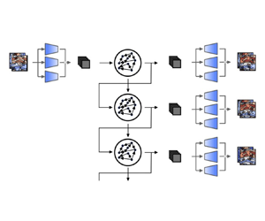
Figure 3. Schematic representation of the closed-loop evolution of the ESN in the latent space, which is decompressed by the decoder.
The ESN can be run either in open-loop or closed-loop configuration. In the open-loop configuration, we feed the data as the input at each time step to compute the reservoir dynamics,  $\boldsymbol {r}(t_i)$. We use the open-loop configuration for washout and training. Washout is the initial transient of the network, during which we do not compute the output, $\hat {\boldsymbol {z}}(t_{i+1})$. The purpose of washout is for the reservoir state to become (i) up-to-date with respect to the current state of the system and (ii) independent of the arbitrarily chosen initial condition, $\boldsymbol {r}(t_0) = {0}$ (echo state property). After washout, we train the output matrix, $\boldsymbol{\mathsf{W}}_{{out}}$, by minimising the MSE between the outputs and the data over the training set. Training the network on $N_{{tr}} + 1$ snapshots consists of solving the linear system (ridge regression)
 \begin{equation} \Big(\boldsymbol{\mathsf{R}}\boldsymbol{\mathsf{R}}^T + \beta \boldsymbol{\mathsf{I}}\Big)\boldsymbol{\mathsf{W}}_{{out}} = \boldsymbol{\mathsf{R}} \boldsymbol{\mathsf{Z}}_{{d}}^T, \end{equation}
where  $\boldsymbol{\mathsf{R}}\in \mathbb {R}^{(N_r+1)\times N_{{tr}}}$ and $\boldsymbol{\mathsf{Z}}_{{d}}\in \mathbb {R}^{N_{{lat}}\times N_{{tr}}}$ are the horizontal concatenations of the reservoir states with bias, $[\boldsymbol {r};1]$, and of the output data, respectively; $\boldsymbol{\mathsf{I}}$ is the identity matrix and $\beta$ is the Tikhonov regularisation parameter (Tikhonov et al. Reference Tikhonov, Goncharsky, Stepanov and Yagola2013). In the closed-loop configuration (figure 3), starting from an initial data point as an input and an initial reservoir state obtained through washout, the output, $\hat {\boldsymbol {z}}$, is fed back to the network as an input for the next time step prediction. In doing so, the network is able to autonomously evolve in the future. After training, the closed-loop configuration is deployed for validation and test on unseen dynamics.
3.2.1. Validation
During validation, we use part of the data to select the hyperparameters of the network by minimising the error of the prediction with respect to the data. In this work, we optimise the input scaling,  $\sigma _{{in}}$, spectral radius, $\rho$, and Tikhonov parameter, $\beta$, which are the key hyperparameters for the performance of the network (Lukoševičius Reference Lukoševičius2012). We use a Bayesian optimisation to select $\sigma _{{in}}$ and $\rho$, and perform a grid search within $[\sigma _{{in}},\rho ]$ to select $\beta$ (Racca & Magri Reference Racca and Magri2021). The range of the hyperparameters vary as a function of the testcase (see the supplementary material). In addition, we add to the training inputs, $\boldsymbol {z}_{tr}$, Gaussian noise, $\mathcal {N}$, with a zero mean and standard deviation, such that $z_{tr_i} = z_i + \mathcal {N}(0,k_z\sigma (z_i))$, where $\sigma ({\cdot })$ is the standard deviation and $k_z$ is a tunable parameter (Appendix D). Adding noise to the data improves the ESN forecasting of chaotic dynamics because the network explores more regions around the attractor, thereby becoming more robust to errors (Lukoševičius Reference Lukoševičius2012; Vlachas et al. Reference Vlachas, Pathak, Hunt, Sapsis, Girvan, Ott and Koumoutsakos2020; Racca & Magri Reference Racca and Magri2022a).
To select the hyperparameters, we employ the recycle validation (RV) (Racca & Magri Reference Racca and Magri2021). The RV is a tailored validation strategy for the prediction of dynamical systems with RNNs, which has been shown to outperform other validation strategies, such as the single shot validation (SSV), in the prediction of chaotic flows (more details are given in Appendix D). In the RV, the network is trained only once on the entire dataset, and validation is performed on multiple intervals already used for training. This is possible because RNNs operate in two configurations (open-loop and closed-loop), which means that the networks can be validated in closed-loop on data used for training in open-loop.
4. Spatial reconstruction
We analyse the ability of the autoencoder to create a reduced-order representation of the flowfield, i.e. the latent space. The focus is on the spatial reconstruction of the flow. Prediction in time is discussed in §§ 5–6.
4.1. Reconstruction error
The autoencoder maps the flowfield onto the latent space and then reconstructs the flowfield based on the information contained in the latent space variables. The reconstructed flowfield (the output) is compared with the original flowfield (the input). The difference between the two flowfields is the reconstruction error, which we quantify with the normalised root-mean-squared error (NRMSE)
 \begin{equation} \mathrm{NRMSE}(\boldsymbol{q}) = \sqrt{\dfrac{\displaystyle\sum\limits_i^{N_{{phys}}} \dfrac{1}{N_{{phys}}} (\hat{q}_i-q_{i})^2 }{\displaystyle\sum\limits_i^{N_{{phys}}} \dfrac{1}{N_{{phys}}}\sigma(q_i)^2}}, \end{equation}
where  $i$ indicates the $i$th component of the physical flowfield, $\boldsymbol {q}$, and the reconstructed flowfield, $\hat {\boldsymbol {q}}$, and $\sigma ({\cdot })$ is the standard deviation. We compare the results for different sizes of the latent space with the reconstruction obtained by POD (Lumley Reference Lumley1970), also known as principal component analysis (Pearson Reference Pearson1901). In POD, the $N_{{lat}}$-dimensional orthogonal basis that spans the reduced-order space is given by the eigenvectors $\boldsymbol {\varPhi }^{({phys})}_i$ associated with the largest $N_{{lat}}$ eigenvalues of the covariance matrix, $\boldsymbol{\mathsf{C}}=({1}/({N_t-1}))\boldsymbol{\mathsf{Q}}_{\boldsymbol{\mathsf{d}}}^T\boldsymbol{\mathsf{Q}}_{\boldsymbol{\mathsf{d}}}$, where $\boldsymbol{\mathsf{Q}}_{\boldsymbol{\mathsf{d}}}$ is the vertical concatenation of the $N_t$ flow snapshots available during training, from which the mean has been subtracted. Both POD and the autoencoder minimise the same loss function (3.3). However, POD provides the optimal subspace onto which linear projections of the data preserve its energy. On the other hand, the autoencoder provides a nonlinear mapping of the data, which is optimised to preserve its energy. (In the limit of linear activation functions, autoencoders perform similarly to POD (Baldi & Hornik Reference Baldi and Hornik1989; Milano & Koumoutsakos Reference Milano and Koumoutsakos2002; Murata et al. Reference Murata, Fukami and Fukagata2020).) The size of the latent space of the autoencoder is selected to be larger than the Kaplan–Yorke dimension, which is $N_{KY} = \{3, 9.5\}$ for the quasiperiodic and turbulent testcases, respectively (§ 2.1). We do so to account for the (nonlinear) approximation introduced by the CAE-ESN, and numerical errors in the optimisation of the architecture.
Figure 4 shows the reconstruction error over 600 000 snapshots (for a total of  $2\times 10^6$ snapshots between the two regimes) in the test set. We plot the results for POD and the autoencoder through the energy (variance) captured by the modes
 \begin{equation} \mathrm{Energy}=1-\overline{\mathrm{NRMSE}}^2, \end{equation}
where  $\overline {\mathrm {NRMSE}}$ is the time-averaged NRMSE. The rich spatial complexity of the turbulent flow (figure 4b), with respect to the quasiperiodic solution (figure 4a), is apparent from the magnitude and slope of the reconstruction error as a function of the latent space dimension. In the quasiperiodic case, the error is at least one order of magnitude smaller than the turbulent case for the same number of modes, showing that fewer modes are needed to characterise the flowfield. In both cases, the autoencoder is able to accurately reconstruct the flowfield. For example, in the quasiperiodic and turbulent cases the nine-dimensional autoencoder latent space captures $99.997\,\%$ and $99.78\,\%$ of the energy, respectively. The nine-dimensional autoencoder latent space provides a better reconstruction than 100 POD modes for the same cases. Overall, the autoencoder provides an error at least two orders of magnitude smaller than POD for the same size of the latent space. These results show that the nonlinear compression of the autoencoder outperforms the optimal linear compression of POD.

Figure 4. Reconstruction error in the test set as a function of the latent space size in (a) the quasiperiodic case and (b) the chaotic case for POD and the CAE.
4.2. Autoencoder principal directions and POD modes
We compare the POD modes provided by the autoencoder reconstruction,  $\boldsymbol {\varPhi }^{({phys})}_{{Dec}}$, with the POD modes of the data, $\boldsymbol {\varPhi }^{({phys})}_{{True}}$. We do so to interpret the reconstruction of the autoencoder as compared with POD. For brevity, we limit our analysis to the latent space of 18 variables in the turbulent case. We decompose the autoencoder latent dynamics into proper orthogonal modes, $\boldsymbol {\varPhi }^{({lat})}_i$, which we name ‘autoencoder principal directions’ to distinguish them from the POD modes of the data. Figure 5(a) shows that four principal directions are dominant, as indicated by the change in slope of the energy, and that they contain roughly $97\,\%$ of the energy of the latent space signal. We therefore focus our analysis on the four principal directions, from which we obtain the decoded field
 \begin{equation} \boldsymbol{\hat{q}}_{{Dec}4}(t) = \boldsymbol{f}\left(\sum_{i=1}^4 a_i(t) \boldsymbol{\varPhi}^{({lat})}_i\right), \end{equation}
where  $a_i(t) = \boldsymbol {\varPhi }^{({lat})T}_i\boldsymbol {z}(t)$ and $\boldsymbol {f}({\cdot })$ is the decoder (§ 3.1). The energy content in the reconstructed flowfield is shown in figure 5(b). On the one hand, the full latent space, which consists of 18 modes, reconstructs accurately the energy content of the first 50 POD modes. On the other hand, $\boldsymbol {\hat {q}}_{{Dec}4}$ closely matches the energy content of the first few POD modes of the true flow field, but the error increases for larger numbers of POD modes. This happens because $\boldsymbol {\hat {q}}_{{Dec}4}$ contains less information than the true flow field, so that fewer POD modes are necessary to describe it. The results are further corroborated by the scalar product with the physical POD modes of the data (figure 6). The decoded field obtained from all the principal components accurately describes the majority of the first 50 physical POD modes, and $\boldsymbol {\hat {q}}_{{Dec}4}$ accurately describes the first POD modes. These results indicate that only few nonlinear modes contain information about several POD modes.

Figure 5. (a) Energy as a function of the latent space principal directions and (b) energy as a function of the POD modes in the physical space for the field reconstructed using 4 and 18 (all) latent space principal direction and data (True).

Figure 6. Scalar product of the POD modes of the data with (a) the POD modes of the decoded flowfield obtained from all the principal directions and (b) the POD modes of the decoded flowfield obtained from four principal directions.
A visual comparison of the most energetic POD modes of the true flow field and of  $\boldsymbol {\hat {q}}_{{Dec}4}$ is shown in figure 7. The first eight POD modes are recovered accurately. The decoded latent space principal directions, $\boldsymbol {f}(\boldsymbol {\varPhi }^{({lat})}_i)$, are plotted in figure 8. We observe that the decoded principal directions are in pairs as the linear POD modes, but they differ significantly from any of the POD modes of figure 7. This is because each mode contains information about multiple POD modes, since the decoder infers nonlinear interactions among the POD modes. Further analysis of the modes and the latent space requires tools from Riemann geometry (Magri & Doan Reference Magri and Doan2022). This is beyond the scope of this study.

Figure 7. POD modes, one per row, for (a) the reconstructed flow field based on four principal components in latent space and (b) the data. Even modes are shown in the supplementary material. The reconstructed flow contains the first eight modes.

Figure 8. Decoded four principal directions in latent space.
5. Time-accurate prediction
Once the autoencoder is trained to provide the latent space, we train an ensemble of 10 ESNs to predict the latent space dynamics. We use an ensemble of networks to take into account the random initialisation of the input and state matrices (Racca & Magri Reference Racca and Magri2022a). We predict the low-dimensional dynamics to reduce the computational cost, which becomes prohibitive when time-accurately predicting high-dimensional systems with RNNs (Pathak et al. Reference Pathak, Hunt, Girvan, Lu and Ott2018a; Vlachas et al. Reference Vlachas, Pathak, Hunt, Sapsis, Girvan, Ott and Koumoutsakos2020). Figure 9 shows the computational time required to forecast the evolution of the system by solving the governing equations and using the CAE-ESN. The governing equations are solved using a single GPU Nvidia Quadro RTX 4000, whereas the CAE-ESN uses a single CPU Intel i7-10700K (ESN) and single GPU Nvidia Quadro RTX 4000 (decoder) in sequence. The CAE-ESN is two orders of magnitude faster than solving the governing equations because the ESNs use sparse matrix multiplications and can advance in time with a  $\delta t$ larger than the numerical solver (see chapter 3.4 of Racca Reference Racca2023).

Figure 9. Computational time required to forecast the evolution of the system for one time unit. Times for the CAE-ESN are for the largest size of the reservoir, which takes the longest time.
5.1. Quasiperiodic case
We train the ensemble of ESNs using 15 000 snapshots equispaced by  $\delta t = 1$. The networks are validated and tested in closed-loop on intervals lasting 500 time units. One closed-loop prediction of the average and local dissipation rates (2.3a,b) in the test set are plotted in figure 10. The network accurately predicts the two quantities for several oscillations (figure 10a,b). The CAE-ESN accurately predicts the entire 4608-dimensional state (see figure 3) for the entire interval, as shown by the NRMSE for the state in figure 10(c).

Figure 10. Prediction of (a) the local and (b) the average dissipation rate in the quasiperiodic case in the test set, i.e. unseen dynamics, for a CAE-ESN with a 2000 neurons reservoir and 9-dimensional latent space.
Figure 11 shows the quantitative results for different latent spaces and reservoir sizes. We plot the percentiles of the network ensemble for the mean over 50 intervals in the test set,  $\langle \cdot \rangle$, of the time-averaged NRMSE. The CAE-ESN time-accurately predicts the system in all cases analysed, except for small reservoirs in large latent spaces (figure 11c,d). This is because larger reservoirs are needed to accurately learn the dynamics of larger latent spaces. For all the different latent spaces, the accuracy of the prediction increases with the size of the reservoir. For 5000 neurons reservoirs, the NRMSE for the prediction in time is the same order of magnitude as the NRMSE of the reconstruction (figure 4). This means that the CAE-ESN learns the quasiperiodic dynamics and accurately predicts the future evolution of the system for several characteristic timescales of the system.

Figure 11. The 25th, 50th and 75th percentiles of the average NRMSE in the test set as a function of the latent space size and reservoir size in the quasiperiodic case.
5.2. Turbulent case
We validate and test the networks for the time-accurate prediction of the turbulent dynamics against the prediction horizon (PH), which, in this paper, is defined as the time interval during which the NRMSE (4.1) of the prediction of the network with respect to the true data is smaller than a user-defined threshold,  $k$
$k$
 \begin{equation} \mathrm{PH} = \mathop{\mathrm{argmax}}\limits_{t_p}(t_p \,|\, \mathrm{NRMSE}(\boldsymbol{q}) < k), \end{equation}
where  $t_p$ is the time from the start of the closed-loop prediction and $k=0.3$. The PH is a commonly used metric, which is tailored for the data-driven prediction of diverging trajectories in chaotic (turbulent) dynamics (Pathak et al. Reference Pathak, Wikner, Fussell, Chandra, Hunt, Girvan and Ott2018b; Vlachas et al. Reference Vlachas, Pathak, Hunt, Sapsis, Girvan, Ott and Koumoutsakos2020). The PH is evaluated in LTs (§ 2). (The PH defined here is specific for data-driven prediction of chaotic dynamics, and differs from the definition of Kaiser et al. (Reference Kaiser2014).)
Figure 12(a) shows the prediction of the dissipation rate in an interval of the test set, i.e. on data not seen by the network during training. The predicted trajectory closely matches the true data for about 3 LTs. Because the tangent space of chaotic attractors is exponentially unstable, the prediction error ultimately increases with time (figure 12b). To quantitatively assess the performance of the CAE-ESN, we create 20 latent spaces for each of the latent space sizes  $[18,36,54]$. Because we train 10 ESNs per each latent space, we analyse results from 600 different CAE-ESNs. Each latent space is obtained by training autoencoders with different random initialisations and optimisations of the weights of the convolutional layers (§ 3.1). The size of the latent space is selected to be larger than the Kaplan–Yorke dimension of the system, $N_{KY} = 9.5$ (§ 2.1), in order to contain the attractor's dynamics. In each latent space, we train the ensemble of 10 ESNs using 60 000 snapshots equispaced by $\delta t =0.5$. Figure 13 shows the average PH over 100 intervals in the test set for the best performing latent space of each size. The CAE-ESN successfully predicts the system for up to more 1.5 LTs for all sizes of the latent space. Increasing the reservoir size slightly improves the performance with a fixed latent space size, whilst latent spaces of different sizes perform similarly. This means that small reservoirs in small latent spaces are sufficient to time-accurately predict the system.

Figure 12. Prediction of the dissipation rate in the turbulent case in the test set, i.e. unseen dynamics, for a CAE-ESN with a 10 000 neurons reservoir and 36-dimensional latent space. The vertical line in panel (a) indicates the PH.

Figure 13. The 25th, 50th and 75th percentiles of the average PH in the test set as a function of the latent space and reservoir size in the turbulent case.
A detailed analysis of the performance of the ensemble of the latent spaces of the same size is shown in figure 14. Figure 14(a) shows the reconstruction error. The small amplitude of the errorbars indicates that different autoencoders with same latent space size reconstruct the flowfield with similar energy. Figure 14(b) shows the performance of the CAE-ESN with 10 000 neurons reservoirs for the time-accurate prediction as a function of the reconstruction error. In contrast to the error in figure 14(a), the PH varies significantly, ranging from 0.75 to more than 1.5 LTs in all latent space sizes. There is no discernible correlation between the PH and reconstruction error. This means that the time-accurate performance depends more on the training of the autoencoder than the latent space size. To quantitatively assess the correlation between two quantities,  $[\boldsymbol {a_1},\boldsymbol {a_2}]$, we use the Pearson correlation coefficient (Galton Reference Galton1886; Pearson Reference Pearson1895)
 \begin{equation} r(\boldsymbol{a_1},\boldsymbol{a_2}) = \frac{\displaystyle \sum (a_{1_i}-\langle a_1 \rangle)(a_{2_i}-\langle a_2 \rangle)} {\displaystyle \sqrt{\sum (a_{1_i}-\langle a_1 \rangle)^2}\sqrt{\sum (a_{2_i}- \langle a_2 \rangle)^2}}. \end{equation}
The values  $r=\{-1,0,1\}$ indicate anticorrelation, no correlation and correlation, respectively. The Pearson coefficient between the reconstruction error and the PH is $r=-0.10$ for the medians of the 60 cases analysed in figure 14(b), which means that the PH is weakly correlated with the reconstruction error. This indicates that latent spaces that similarly capture the energy of the system, may differ in capturing the dynamical content of the system; i.e. some modes that are critical for the dynamical evolution of the system do not necessarily affect the reconstruction error, and therefore may not necessarily be captured by the autoencoder. This is a phenomenon that also affects different reduced-order modelling methods, specifically POD (Rowley & Dawson Reference Rowley and Dawson2017; Agostini Reference Agostini2020). In figure 14(c), we plot the PH of the medians of the errorbars of figure 14(b) for different latent spaces. Although the performance varies within the same size of the latent space, we observe that the PH improves and the range of the errorbars decreases with increasing size of the latent space. This is because autoencoders that better approximate the system in a $L_2$ sense are also more likely to include relevant dynamical information for the time evolution of the system. From a design perspective, this means that latent spaces with smaller reconstruction error are needed to improve and reduce the variability of the prediction of the system. A different approach, which is beyond the scope of this paper, is to generate latent spaces tailored for time-accurate prediction (a more detailed discussion can be found in the supplementary material).

Figure 14. The 25th, 50th and 75th percentiles of (a) the reconstruction error of figure 4 from twenty different latent spaces of different size, (b) the PH as a function of the reconstruction error and (c) the medians of the PH of (b) as a function of the latent space size. The line in (b) is obtained by linear regression.
6. Statistical prediction
We analyse the statistics predicted by the CAE-ESN with long-term predictions. Long-term predictions are closed-loop predictions that last tens of LTs, whose instantaneous state differs from the true data because of chaos (infinitesimal errors exponentially grow in chaotic systems). However, in ergodic systems, the trajectories evolve within a bounded region of the phase space, the attractor, which means that they share the same long-term statistics. The long-term predictions are generated from 50 different starting snapshots in the training set. In the quasiperiodic case, each time series is obtained by letting the CAE-ESN evolve in closed-loop for 2500 time units, whereas in the chaotic case the CAE-ESN evolves for 30 LTs. (If the network predicts values outside the range of the training set, we discard the remaining part of the closed-loop prediction, similarly to Racca & Magri (Reference Racca and Magri2022a).) To quantify the error of the predicted probability density function (p.d.f.) with respect to the true p.d.f., we use the first-order Kantorovich metric (Kantorovich Reference Kantorovich1960), also known as the Wasserstein distance or Earth mover's distance. The Kantorovich metric evaluates the work to transform one p.d.f. to another, which is computed as
 \begin{equation} \mathcal{K} = \int_{-\infty}^{\infty}|\mathrm{CDF}_1(k) - \mathrm{CDF}_2(k)|\,{\rm d}k, \end{equation}
where  $\mathrm {CDF}$ is the cumulative distribution function and $k$ is the random variable of interest. Small values of $\mathcal {K}$ indicate that the two p.d.f.s are similar to each other, whereas large values of $\mathcal {K}$ indicate that the two p.d.f.s significantly differ from each other.
6.1. Quasiperiodic case
To predict the statistics of the quasiperiodic case, we train the network on small datasets. We do so because the statistics are converged for the large dataset (15 000 time units) used for training in § 5 (figure 15a). We use datasets with non-converged statistics to show that we can infer the converged statistics of the system from the imperfect data available during training. We analyse the local dissipation rate at the central point of the domain,  $d_{{\rm \pi},{\rm \pi} }$, which shows quasiperiodic oscillations (§ 2). Figure 15(b) shows the Kantorovich metric for the CAE-ESN as a function of the number of training snapshots in the dataset for fixed latent space and reservoir size. The networks improve the statistical knowledge of the system with respect to the training set, i.e. the original data, in all cases analysed, which generalises the findings of Racca & Magri (Reference Racca and Magri2022a) to spatiotemporal systems. The improvement is larger in smaller datasets, and it saturates for larger datasets. This means that (i) the networks accurately learn the statistics from small training sets and (ii) the networks are able to extrapolate from imperfect statistical knowledge and provide an accurate estimation of the true statistics. Figure 16 shows the performance of the CAE-ESN as a function of the reservoir size for the small dataset of 1500 training snapshots. In all cases analysed, the CAE-ESN outperforms the training set, with values of the Kantorovich metric up to three times smaller than those of the training set. Consistently with previous studies on ESNs (Huhn & Magri Reference Huhn and Magri2022; Racca & Magri Reference Racca and Magri2022a), the performance is approximately constant for different reservoir sizes. The results indicate that small reservoirs and small latent spaces are sufficient to accurately extrapolate the statistics of the flow from imperfect datasets.

Figure 15. (a) P.d.f. of the local dissipation rate,  $d_{{\rm \pi},{\rm \pi} }$, in the training set for different numbers of training snapshots. (b) The 25th, 50th and 75th percentiles of the Kantorovich metric for the training set (Train) and for the CAE-ESN (Predicted) as a function of the training set size. Quasiperiodic regime.

Figure 16. The 25th, 50th and 75th percentiles of the Kantorovich metric of the local dissipation rate,  $d_{{\rm \pi},{\rm \pi} }$, for the training set (Train) and for the networks (Predicted) as a function of the latent space and reservoir size in the quasiperiodic case.
6.2. Turbulent case
In the turbulent case, we analyse the ability of the architecture to replicate the p.d.f. of the average dissipation rate,  $D$, to assess whether the networks have learned the dynamics in a statistical sense. Figure 17 shows the results for the best performing CAE-ESN with latent space of size 18, 36 and 54 discussed in § 5. Figure 17(a) shows the Kantorovich metric as a function of the size of the reservoir. The networks predict the statistics of the dissipation rate with Kantorovich metrics of the same order of magnitude of the training set, which has nearly converged statistics. This means that the network accurately predict the p.d.f. of the dissipation rate (figure 17b). In agreement with the quasiperiodic case, the performance of the networks is approximately constant as a function of the reservoir size. These results indicate that small latent spaces and small networks can learn the statistics of the system.

Figure 17. (a) The 25th, 50th and 75th percentiles of the Kantorovich metric of the dissipation rate, for the training set (Train) and for different reservoir and latent space sizes. (b) P.d.f. for the true and training data, and predicted by 10 000 neurons CAE-ESNs.
A detailed analysis of the statistical performance of the 20 latent spaces of size  $[18,36,54]$ is shown in figure 18. On the one hand, figure 18(a) shows the scatter plot between the Kantorovich metric and the reconstruction error. In agreement with the results for the PH (see figure 14), we observe that (i) the Kantorovich metric varies significantly within latent spaces of the same size, (ii) the two quantities are weakly correlated ( $r=-0.16$) and (iii) the variability of the performance decreases with increasing latent space size (figure 18c). On the other hand, figure 18(b) shows the scatter plot for the Kantorovich metric as a function of the PH, which represents the correlation between the time-accurate and statistical performances of the networks. The two quantities are (anti)correlated, with a Pearson coefficient $r=-0.76$. Physically, the results indicate that (i) increasing the size of the latent space is beneficial for predicting the statistics of the system and (ii) the time-accurate and statistical performances of latent spaces are correlated. This means that the design guidelines for the time-accurate prediction discussed in § 5 extend to the design of latent spaces for the statistical prediction of turbulent flowfields.

Figure 18. (a) The 25th, 50th and 75th percentiles for the Kantorovich metric as a function of the reconstruction error, (b) medians of the Kantorovich metric as a function of the median of the PH and (c) the 25th, 50th and 75th percentiles of the medians of the Kantorovich metric of (b) as a function of the latent space. The lines in (a,b) are obtained by linear regression.
7. Predicting higher-dimensional turbulence: the minimal flow unit
Because of its relatively small size, the two-dimensional Kolmogorov flow (§ 2) enables us to thoroughly assess the accuracy and robustness of the proposed method with a variety of parametric and ensemble computations. In this section, we explain how to modify the CAE-ESN to tackle three-dimensional fields. We deploy the CAE-ESN for the statistical prediction of the minimal flow unit (MFU) (Jimenez & Moin Reference Jimenez and Moin1991). This flow is governed by the incompressible Navier–Stokes equations, presented in § 2, with velocity  $\boldsymbol {u}=(u,v,w)$. As shown in figure 19, the MFU consists of a channel flow-like configuration with no-slip boundary conditions in the wall-normal direction, $y$, at $\boldsymbol {u}(x,\pm \delta,z,t)=0$, where $\delta$ is the half-width of the channel, and periodic boundary conditions in the streamwise, $x$, and transverse, $z$, directions. The flow is forced with a body forcing $\boldsymbol {f}=(f_0,0,0)$ in the streamwise direction. We consider a channel of dimension ${\rm \pi} \delta \times 2\delta \times 0.34{\rm \pi} \delta$ with $\delta =1.0$ and a forcing term that provides a friction Reynolds number, $Re_\tau \approx 140$ as in Blonigan, Farazmand & Sapsis (Reference Blonigan, Farazmand and Sapsis2019). These conditions result in a turbulent flow, as shown in figure 19. We use an in-house direct numerical simulation (DNS) code based on work by Bernardini, Pirozzoli & Orlandi (Reference Bernardini, Pirozzoli and Orlandi2014) to simulate the MFU on a grid $32 \times 256 \times 16$, yielding a $32 \times 256 \times 16 \times 3 \approx 4\times 10^5$-dimensional physical state vector. We solve the equations using a hybrid third-order low-storage Runge–Kutta algorithm coupled with a second-order Crank–Nicolson scheme (Bernardini et al. Reference Bernardini, Pirozzoli and Orlandi2014). The timestep is computed at the initial state to ensure the stability of the numerical scheme (initial Courant–Friedrichs–Lewy (CFL) number of 2/3), and is subsequently kept constant to a value approximately equal to 1/100 of the eddy turnover time. After removing the transient dynamics, snapshots are saved every 10 timesteps for a total of 2000 snapshots covering approximately 200 eddy turnover times. To train the three-dimensional version of the CAE-ESN, we split the dataset for training/validation/test as 60/20/20.

Figure 19. (a) Typical snapshot of the isosurfaces of the  $Q$-criterion in the MFU. (b) Reconstruction error in the test set as a function of the latent space size for the MFU case.
We describe the adjustments made to the CAE-ESN presented in § 3 to enable it to handle three-dimensional flows. In the encoder part of the CAE, instead of using two-dimensional convolutional layers, three-dimensional convolutional layers are used. Periodic padding is only used in the  $x$- and $z$-directions, while zero padding is used in the $y$-direction. This padding is physically consistent with the boundary conditions. Similarly, in the decoder part of the CAE, three-dimensional transpose convolutional layers are employed. To balance the size of the CAE and reconstruction accuracy, only two parallel encoder/decoder streams are used in the multiscale autoencoder architecture, which have spatial filter sizes $3\times 5 \times 3$ and $5 \times 7 \times 5$, respectively. For the reducing/increasing size layers, a striding of the form $(2,4,2)$ is used. Details on the CAE architecture are provided in Appendix C. The CAE is trained using the same method as described in § 3.1. The architecture of the ESN is identical to the architecture presented in § 3.2, but with a reservoir containing 150 000 neurons. The hyperparameters of the ESN are obtained using the RV (Racca & Magri Reference Racca and Magri2021), in which the training dataset is the encoded MFU evolution.
Figure 19(b) shows the performance of the CAE through the reconstruction error discussed in § 4. The energy for POD and three different CAEs, with latent space dimensions of 384, 768, 1536 and 3072, respectively, is computed over the 400 snapshots in the test set, similarly to figure 4 in the Kolmogorov flow. The CAE outperforms POD, with POD requiring, for example, approximately 10 times larger latent spaces to obtain the same reconstruction error as the CAE with 1536-dimensional latent space. The performance of the combined CAE-ESN, with a CAE of latent dimension 1536, is finally assessed statistically in figure 20. This latent dimension was chosen as it provided sufficient reconstruction accuracy in the CAE. We perform long-term predictions of the CAE-ESN for a duration of 100 eddy turnover times, and compare the resulting mean and fluctuating velocity profiles with the true DNS data. The CAE-ESN correctly predicts the true mean (figure 20a) and fluctuating velocity profiles (figure 20b) of the MFU. In conclusion, the CAE-ESN can statistically learn and predict the dynamics of three-dimensional turbulent flows through relatively small latent spaces.

Figure 20. Profile of (a) mean streamwise and (b) fluctuating streamwise and wall-normal velocity profiles. Grey line: true statistics. Red/blue dashed lines: statistics from the CAE-ESN.
8. Conclusions
In this paper, we propose the CAE-ESN for the prediction of two- and three-dimensional turbulent flowfields from data. The CAE nonlinearly maps the flowfields onto (and back from) the latent space, whose dynamics are predicted by an ESN. We assess the capabilities of the CAE-ESN methodology on a variety of studies on a two-dimensional flowfield, in both quasiperiodic and turbulent regimes. The CAE-ESN is finally deployed to predict the statistics of a three-dimensional turbulent flow. First, we show that the CAE-ESN time-accurately and statistically predicts the flow. The latent space requires  ${\lesssim }1\,\%$ of the degrees of freedom of the original flowfield. In the prediction of the spatiotemporal dynamics, the CAE-ESN is at least 100 times faster than solving the governing equations. This is possible thanks to the nonlinear compression provided by the autoencoder, which has a reconstruction error that is ${\lesssim }1\,\%$ of that from POD. Second, we analyse the performance of the architecture at different Reynolds numbers. The architecture correctly learns the dynamics of the system in both quasiperiodic and turbulent testcases. This means that the architecture is robust with respect to changes in the physical parameters of the system. Third, we analyse the performance of the CAE-ESN as a function of the reconstruction error. We show that (i) the performance varies between latent spaces with similar reconstruction error, (ii) larger latent spaces with smaller reconstruction errors provide a more consistent and more accurate prediction on average and (iii) the time-accurate and statistical performance of the CAE-ESN are correlated. This means that relatively small reservoirs in relatively small latent spaces are sufficient to time-accurately and statistically predict the turbulent dynamics, and increasing the latent space size is beneficial for the performance of the CAE-ESN. Finally, we extend the CAE-ESN to three-dimensional turbulent flows. By analysing the MFU as a testcase, we show that POD requires a latent space that is approximately 10 times larger than the latent space inferred by the CAE-ESN for the same reconstruction error. By letting the CAE-ESN evolve as an autonomous dynamical system, the turbulent velocity statistics of the MFU are accurately inferred. By proposing a data-driven framework for the nonlinear decomposition and prediction of turbulent dynamics, this paper opens up possibilities for nonlinear reduced-order modelling of turbulent flows.
Supplementary material
Supplementary material is available at https://doi.org/10.1017/jfm.2023.716 (and also at https://link.springer.com/chapter/10.1007/978-3-030-77977-1_25).
Funding
A.R. is supported by the Engineering and Physical Sciences Research Council under the Research Studentship no. 2275537, by the Cambridge Commonwealth, European & International Trust under a Cambridge European Scholarship, and by the Eric and Wendy Schmidt AI in Science Postdoctoral Fellowship, a Schmidt Futures program. L.M. gratefully acknowledges financial support from the ERC Starting Grant PhyCo 949388. The authors are grateful to D. Kelshaw for helpful discussions on the numerical solver. L.M. and N.A.K.D. acknowledge computational resources received from the Stanford University CTR Summer Program 2022.
Declaration of interests
The authors report no conflict of interest.
Appendix A. Tutorial codes
Sample codes and datasets for this work are publicly available on GitHub, in which we include a tutorial implementation of the CAE-ESN. This takes  $\approx$15 min to be trained on a single CPU Intel i7-10700K (ESN) and single GPU Quadro RTX 4000.
Appendix B. Characterisation of the Kolmogorov flow
In this appendix, we provide additional details on the solutions of the Kolmogorov flow. Figure 21 shows the power spectral density of the local and global dissipation in the quasiperiodic regime. As explained in figure 1, the global dissipation is periodic, while the local dissipation is quasiperiodic. This happens because temporal frequencies are filtered out when averaging in space. In more detail, the quasiperiodic solution discussed here presents three incommensurate frequencies, given by the two left-most peaks and the peak shared with the periodic signal (figure 21).

Figure 21. Power spectral density for  $Re=30$.
Appendix C. Autoencoder layers
We provide additional details about the autoencoder described in § 3.1 in table 1. The total number of trainable parameters of the autoencoder is around 200 000 (the exact number varies depending on the size of the latent space). In the table, the explanation ‘Each scale has different padding size’ indicates that different filter sizes, i.e. the different scales of the autoencoder, require different padding sizes in order for their output to have the same size. In reference to figure 2(b), a  $2\times 2$ filter with $\textrm {stride} = 1$ requires padding $\textrm {size} = 1$ for the output of the convolution to be of size $3\times 3$; a $3\times 3$ filter with $\textrm {stride} = 1$ would require padding $\textrm {size} = 3$ for the output of the convolution to be of size $3\times 3$ (for padding sizes larger than 1, the padding is applied symmetrically to both sides of the inputs).
Table 1. Autoencoder layers. Output size differs from one scale to the other, here we show those relative to the  $3\times 3$ filter.

Table 2. Autoencoder layers for the MFU. Output size differs from one scale to the other, here we show those relative to the  $3\times 5 \times 3$ filter.

Appendix D. ESN hyperparameters
We provide additional details regarding the selection of hyperparameters in ESNs. In the quasiperiodic case, we explore the hyperparameter space  $[0.01,5]\times [0.8,1.2]$ for $[\sigma _{{in}},\rho ]$ in logarithmic scale for the input scaling. We optimise the spectral radius in the range around unity from previous studies with quasiperiodic data (Racca & Magri Reference Racca and Magri2021; Nóvoa & Magri Reference Nóvoa and Magri2022). We select the hyperparameters to minimise the average MSE of 30 intervals of length 500 time units taken from the training and validation dataset. To select the noise to be added to the inputs, for each network we perform a search in $k_z$ in points equispaced in logarithmic scale by $\log _{10}(\sqrt {10})$. The search starts by evaluating the average MSE in the test set for $[k_{z1},k_{z2}] = [10^{-3}, \sqrt {10}\times 10^{-3}]$. Based on the slope of the MSE as a function of $k_z$ provided by $[k_{z1},k_{z2}]$, we select $k_{z3}$ to either be $k_{z1}/\sqrt {10}$ or $k_{z2}\times \sqrt {10}$ in order to minimise the MSE. From $[k_{z1},k_{z2}, k_{z3}]$ we select a new point, and so on and forth. The search continues until a local minimum of the MSE is found or the maximum numbers of four function evaluations is reached. In the chaotic case, we explore the hyperparameter space $[0.1,5]\times [0.1,1.]$ for $[\sigma _{{in}},\rho ]$ in logarithmic scale for the input scaling. We select the hyperparameters to maximise the average PH of 50 starting points taken from the training and validation dataset. To select the noise to be added to the inputs, we follow a similar procedure to the quasiperiodic case. However, due to computational constraints related to larger sizes of the reservoir, we perform the search only for the first network of the ensemble and utilise the optimal $k_z$ for all the other networks in the ensemble. The search starts from $[k_{z1},k_{z2}] = [\sqrt {10}\times 10^{-3}, 10^{-2}]$. In both cases, (i) washout consists of 50 steps, (ii) we optimise the grid $[10^{-3}, 10^{-6},10^{-9}]$ for $\beta$ and (iii) the Bayesian optimisation starts from a grid of $5\times 5$ points in the $[\sigma _{{in}},\rho ]$ domain and then selects five additional points through the expected improvement acquisition function (Brochu, Cora & De Freitas Reference Brochu, Cora and De Freitas2010). The Bayesian optimisation is implemented using Scikit-learn (Pedregosa et al. Reference Pedregosa, Varoquaux, Gramfort, Michel, Thirion, Grisel, Blondel, Prettenhofer, Weiss and Dubourg2011).
Finally, this optimisation procedure for both the CAE and the ESN is mainly for fine-tuning. To show this, we provide a tutorial on GitHub, where we train the CAE for only 100 epochs (instead of 2000) and optimise only the spectral radius, input scaling and Tikhonov parameter in the ESN. This simplified architecture accurately predicts the quasiperiodic testcase (results not shown here, available on GitHub). The procedure used to select parameters in the simplified architecture is a robust optimisation method, which has been tested across several chaotic testcases (for example, Racca & Magri Reference Racca and Magri2022a; Nóvoa et al. Reference Nóvoa, Racca and Magri2023; Margazoglou & Magri Reference Margazoglou and Magri2023). In the simplified version, the entire training of the CAE-ESN requires only approximately  $15$ min on a single CPU Intel i7-10700K and single GPU Nvidia Quadro RTX 4000.
We show a comparison of the RV with the SSV in figure 22 for the prediction of the turbulent case. The RV outperforms the SSV, providing an increase of roughly 10 % on average of the 50th percentile of the PH. Moreover, the RV reduces the variability of the performance of different networks of the same size, making the training more robust to the random initialisation of the networks. This results in the average uncertainty given by the width of the error bars is roughly 70 % larger in the SSV with respect to the RV. These results indicate that the RV outperforms and is more reliable than the SSV in the prediction of the turbulent flow.

Figure 22. The 25th, 50th and 75th percentiles of the average PH in the test set for the RV and the SSV.


 Open access