


1. Introduction
Spherical tokamaks (STs) have a significantly smaller aspect ratio, i.e. ratio of plasma major radius ($R_0$ ) to plasma minor radius ($a$
 ), than conventional tokamaks. Their compact shape allows for more efficient confinement at a given magnetic field strength than in conventional tokamaks. The more compact configuration can lower the construction cost and STs have been proposed as component testing facilities, to aid the development of magnetic confinement fusion. However, beyond their use in component testing, there is an effort to construct STs suitable for energy production in order to accelerate the path to commercially available fusion power. Part of this effort is the Spherical Tokamak for Energy Production (STEP) program in the UK, aiming to design and construct a prototype fusion energy plant by 2040 (Wilson et al. Reference Wilson, Chapman, Denton, Morris, Patel, Voss and Waldon2020; UKAEA 2022). One phase in the STEP program has been to develop a preliminary high power ST design to understand the interplay between turbulence and shaping for a STEP reactor equilibrium. This design is called BurST, short for Burning Spherical Tokamak (Patel Reference Patel2021).
One of the remaining challenges of reactor-scale tokamaks is the rare, yet potentially detrimental, occurrence of rapid, unwanted degradation of the plasma magnetic confinement, and associated loss of thermal energy, known as a disruption. In the first phase of a disruption there is a dramatic decrease of the plasma temperature from the initial ${\sim }10\,{\rm keV}$ down to ${\sim }10\,{\rm eV}$
 , within a few milliseconds. This phase is called the thermal quench (TQ), and it is caused by a combination of an elevated radial transport, due to instabilities temporarily destroying magnetic flux surfaces, and atomic physics processes, including radiation by impurities and plasma dilution. Impurities may enter the plasma unintentionally, or could be injected as part of a disruption mitigation scheme. Even though a part of the plasma thermal energy is isotropically radiated away, the remaining fraction, which is transported to the tokamak wall, can be significant. These transported heat loads tend to be very localised, and may damage the plasma-facing components.
As the temperature in the plasma drops during a disruption, the plasma resistivity increases, leading to a decay of the plasma current and characterising the beginning of the second phase of a disruption – the current quench (CQ). As a consequence, currents are induced in the reactor wall leading to structural forces that can be large enough to damage the device. Furthermore, an electric field is induced in the plasma when the plasma current drops, which, if strong enough, can accelerate electrons to relativistic energies. Such electrons are called runaway electrons (REs) and they can severely damage areas upon which they have an uncontrolled impact.
When a disruption occurs, its impact will have to be mitigated so that the tokamak does not suffer substantial damage. The runaway current should be kept below a certain limit in order to avoid unacceptable melting of the wall, and possibly also underlying structures, in the case of localised loss; here, we restrict this limit to be comparable to that in ITER, 150 kA (Lehnen & the ITER DMS task force Reference Lehnen2021), which corresponds to ${\sim }0.7\,\%$ of the initial BurST plasma current. The CQ time $t_\text {CQ}$
 , i.e. the time it takes for the ohmic component of the current to decay, should also be in an acceptable range to avoid excessive mechanical stresses due to eddy currents and halo currents in the wall. Accounting for plasma inductance (Wesley et al. Reference Wesley, Hyatt, Strait, Schissel, Flanagan, Hender, Gribov, de Vries, Fredrickson and Gates2006), the lower limit is expected to be around 20 ms, with a preliminary upper limit of approximately 100 ms, consistent with the time scale of slow vertical displacement events modelled with BurST-like parameters (T. Hender, private communication 2021; note that the preliminary BurST design did not include a full wall description). For reference, the upper limit on ITER is slightly more relaxed; 150 ms (Hollmann et al. Reference Hollmann, Aleynikov, Fülöp, Humphreys, Izzo, Lehnen, Lukash, Papp, Pautasso and Saint-Laurent2015) and the allowable values are not expected to extend far outside this range. Furthermore, the fraction of the thermal energy lost through radial transport during the TQ should remain below a certain value, to avoid unacceptable localised heat loads on the wall. The ITER target for the upper limit of the transported fraction, 10 % (Hollmann et al. Reference Hollmann, Aleynikov, Fülöp, Humphreys, Izzo, Lehnen, Lukash, Papp, Pautasso and Saint-Laurent2015), is also applied here.
One of the methods proposed to mitigate these potentially harmful effects is massive material injection (Hollmann et al. Reference Hollmann, Aleynikov, Fülöp, Humphreys, Izzo, Lehnen, Lukash, Papp, Pautasso and Saint-Laurent2015). Material injection can act to reduce the runaway generation, as the critical energy for electron runaway is higher at an elevated electron density. A suitable material to inject for this purpose is deuterium. Massive material injection can also be used to control the CQ time, as $t_\text {CQ}$ is proportional to the conductivity, which depends on the final temperature after the TQ, and this temperature is in turn determined by an equilibrium between the ohmic heating and impurity radiation. A suitable material to inject for this purpose is thus a radiating impurity species, typically noble gases such as neon or argon. The injected material can also radiate away a large fraction of the thermal energy during the disruption. To accommodate all requirements at once, injection of a mixture of deuterium and a noble gas is preferred. This has the added benefit that the radiation efficiency is enhanced through the increase in electron density offered by the injected deuterium, as the collisional excitation rate depends on the electron density.
Runaway electron generation has been studied extensively for conventional tokamaks. To date, runaways have rarely been observed in STs during the short disruption time scales in the current small devices. The disruption dynamics usually differs from that in a conventional tokamak (Gerhardt, Menard & the NSTX team Reference Gerhardt and Menard2009; Thornton Reference Thornton2011) and it is therefore not straightforward to transfer the results about runaway electron dynamics in conventional tokamaks to STs. ST plasmas are typically strongly elongated, and it has been shown that elongated plasmas in a conventional tokamak produce fewer runaway electrons during disruptions (Fülöp et al. Reference Fülöp, Helander, Vallhagen, Embreus, Hesslow, Svensson, Creely, Howard and Rodriguez-Fernandez2020). The strong magnetic field variation typically produces large trapped particle populations in STs, which may be expected to affect current evolution in unmitigated disruptions. The aim of this paper is therefore to numerically investigate the potential runaway dynamics in reactor-scale STs, using input parameters for the BurST reactor design as a basis. We highlight comparisons with the expected runaway behaviour in a similarly sized conventional aspect ratio tokamak, such as ITER.
2. Disruption and runaway modelling
The results are obtained using the numerical framework dream (Disruption Runaway Electron Analysis Model) (Hoppe, Embreus & Fülöp Reference Hoppe, Embreus and Fülöp2021) that self-consistently evolves background plasma parameters together with the runaway dynamics during a disruption. For our purposes, dream is used in fluid mode, in which the thermal electron bulk, the runaway electrons and the ion species are each treated as fluid species. The various physics mechanisms activated in fluid mode, such as the runaway generation rates, show good correspondence to the more sophisticated kinetic results, with the model included for processes such as Dreicer generation constructed from large kinetic simulation databases (Hesslow et al. Reference Hesslow, Unnerfelt, Vallhagen, Embreus, Hoppe, Papp and Fülöp2019b). We do not require inherently kinetic outputs, such as the phase space distribution function, in this scoping study of ST-based reactor-scale disruptions and can thus take advantage of the much less computationally demanding fluid mode to perform wide parameter explorations.
In the fluid model, the thermal electron bulk is characterised by its density $n_{e}$ , temperature $T_{e}$
 and the ohmic current density parallel to the magnetic field lines $j_\text {ohm}$
 . In our case, $n_{e}$
 represents the density of all free electrons that are not runaways, i.e. $n_{e} = n_\text {free} - n_\text {re}$
 , and as such, it is determined by the evolution of the runaway and free electron densities. The free electron density is determined by the ion composition of the plasma. The density $n_i^{(j)}$
 of ion species $i$
 with charge state $j$
 is evolved according to the ion rate equation

where $\mathcal {I}$ and $\mathcal {R}$
 are ionisation and recombination rates, respectively, which depend on the plasma parameters (Vallhagen et al. Reference Vallhagen, Embreus, Pusztai, Hesslow and Fülöp2020). The ions are assumed to be fully ionised at the start of the simulation, as the plasma is assumed to be representative of steady-state operation before the disruption occurs.
The time evolution of the runaway electron density $n_\text {re}$ is given by

Here, each source term marks the generation rate of the mechanism indicated by its subscript. Dreicer runaway generation is a phenomenon where electrons diffusively leak into the runaway region due to small-angle collisions (Dreicer Reference Dreicer1959). The hot-tail generation mechanism produces runaways due to the fastest electrons not having time to thermalise before the electric field rises, after a sufficiently fast temperature drop during the TQ (Helander et al. Reference Helander, Smith, Fülöp and Eriksson2004; Smith et al. Reference Smith, Helander, Eriksson and Fülöp2005; Svenningsson et al. Reference Svenningsson, Embreus, Hoppe, Newton and Fülöp2021). Tritium in the device undergoes $\beta$ -decay, generating energetic electrons according to a continuous energy spectrum, a part of which may be in the runaway region (Martín-Solís, Loarte & Lehnen Reference Martín-Solís, Loarte and Lehnen2017; Fülöp et al. Reference Fülöp, Helander, Vallhagen, Embreus, Hesslow, Svensson, Creely, Howard and Rodriguez-Fernandez2020). Runaway electrons generated by Compton scattering of $\gamma$
 -rays from the activated wall are not included here, due to the lack of input data for the spectrum of $\gamma$
 -photons emitted from the plasma-facing components in a reactor such as BurST. Finally, close collisions between a runaway electron and a thermal one can transfer sufficient energy to the latter so that it also becomes a runaway electron. This leads to an exponential increase in the number of runaway electrons, with the avalanche multiplication rate $\varGamma _{\text {ava}}$
 (Rosenbluth & Putvinski Reference Rosenbluth and Putvinski1997; Embréus, Stahl & Fülöp Reference Embréus, Stahl and Fülöp2018). The last term of (2.2) describes a diffusive radial transport of REs. For the transport of REs and heat (to be discussed in more detail later), we use a collisionless Rechester–Rosenbluth-type diffusion coefficient (Rechester & Rosenbluth Reference Rechester and Rosenbluth1978) of the form

for particles with parallel velocity $v_{\|}$ , with the normalised magnetic perturbation amplitude $\delta B/B$
 . When evaluating $D_{\rm re}$
 , we assume $v_{\|}=c$
 for all REs. The RE particle transport term is activated only in some simulations with material injection.
Existing analytical expressions for the Dreicer runaway generation rate $\gamma _{\text {Dreicer}}$ neglect the effects of partial screening, which have been shown to be important (Hesslow et al. Reference Hesslow, Embréus, Hoppe, DuBois, Papp, Rahm and Fülöp2018a). We therefore employ the neural network trained on a large number of kinetic simulations presented in Hesslow et al. (Reference Hesslow, Unnerfelt, Vallhagen, Embreus, Hoppe, Papp and Fülöp2019b), which takes the effects of partial screening into account. The energy dependent model for the Coulomb logarithm is described in equation (18) in Hoppe et al. (Reference Hoppe, Embreus and Fülöp2021), which in the fluid mode is evaluated at a representative runaway momentum of $20\,m_{e}c$
 . The model for the tritium decay generation is taken to be as in Fülöp et al. (Reference Fülöp, Helander, Vallhagen, Embreus, Hesslow, Svensson, Creely, Howard and Rodriguez-Fernandez2020). In the model for the hot-tail, an analytic approximate distribution function and critical runaway momentum are calculated as functions of the background plasma parameters and electric field. These are then used to evaluate $\gamma _{\text {hot-tail}}$
 , as described in appendix C.4 of Hoppe et al. (Reference Hoppe, Embreus and Fülöp2021). The avalanche multiplication rate is described in Hesslow et al. (Reference Hesslow, Embréus, Vallhagen and Fülöp2019a), and it accounts for both partial screening and magnetic trapping effects. Magnetic trapping is likely substantial at the outer flux surfaces in tight aspect ratio devices if the collisionality is low. The effect of trapping is accounted for in the evolution of the electron distribution function, as described in detail in appendix C of Hoppe et al. (Reference Hoppe, Embreus and Fülöp2021), and its impact on the simulations presented here is discussed in the next section.
The magnetic geometry is parameterised according to the analytical model described by Miller et al. (Reference Miller, Chu, Greene, Lin-Liu and Waltz1998). In this geometry model, the radial coordinate, $r$ , measures the half-width of a flux surface in the mid-plane. The flux surfaces are parameterised by their elongation $\kappa (r)$
 , Shafranov shift $\Delta (r)$
 , triangularity $\delta (r)$
 and toroidal magnetic field function $G(r)=R B_\varphi (r)$
 . There is, however, one difference compared with the original Miller model, namely that the Shafranov shift is defined to be zero at the magnetic axis (Hoppe et al. Reference Hoppe, Embreus and Fülöp2021). Apart from specifying the above geometrical parameters, the user also inputs the plasma minor radius $a$
 , major radius (at the magnetic axis) $R_0$
 and wall radius $b = a + r_\text {wall}$
 , where $r_\text {wall}$
 is the distance between the plasma edge and the wall.Footnote 1
The evolution of the electron temperature $T_{e}$ is prescribed as an exponential decay in the simulations of unmitigated disruptions, whereas the temperature is self-consistently evolved for the mitigated disruptions. The exponential temperature decay is given by

where $T_0(r)$ is the initial temperature profile, $t_0$
 is the decay time scale and $T_f(r)$
 is the final temperature profile. After a disruption, the final temperature $T_f$
 is usually flatter than the initial $T_0$
 -profile and is therefore taken as a radially constant value, for simplicity. The self-consistent temperature evolution, used in the mitigation simulations, is described by the energy balance equation for the thermal energy density of the bulk electrons $W_{e}$
 , which relates to the temperature through $W_{e} = 3n_{e}T_{e}/2$
 . The energy balance equation takes into account ohmic heating by the electric field, electron heat diffusion, bremsstrahlung radiation losses, line radiation losses and ionisation energy losses (Hoppe et al. Reference Hoppe, Embreus and Fülöp2021). In the mitigation simulations, the injected material is assumed to be present as a neutral gas at the beginning of the disruption, with a radially constant profile.
In the energy balance equation governing temperature evolution, heat transport is included during the material injection simulations. The heat diffusion coefficient is obtained by taking the heat flux moment of (2.3) for a Maxwellian distribution, yielding $D_W \approx 2\sqrt {{\rm \pi} } v_{\text {th},e} R_0 (\delta B/B)^2$ . Whenever heat and RE particle transport are both active, both diffusivities are calculated using the same magnetic perturbation amplitude, $\delta B/B$
 , for consistency. Furthermore, the effect of opacity is included in the mitigation simulations by using ionisation, recombination and radiation rates for the hydrogen isotopes that are based on the assumption of the plasma being opaque to Lyman radiation. This has been shown to significantly affect the results by reducing excessive cooling and recombination, and thereby reducing the avalanche growth rate (Vallhagen et al. Reference Vallhagen, Pusztai, Hoppe, Newton and Fülöp2022).
The total current density is given by $j = j_\text {ohm} + j_\text {re}$ , where $j_ {\text {re}} =e c n_{\text {re}}$
 as the runaway electrons are assumed to move with the speed of light $c$
 parallel to the magnetic field (Hoppe et al. Reference Hoppe, Embreus and Fülöp2021). The evolution of $j$
 is governed by the evolution of the poloidal flux $\psi (r)$
 (Hoppe et al. Reference Hoppe, Embreus and Fülöp2021; Pusztai, Hoppe & Vallhagen Reference Pusztai, Hoppe and Vallhagen2022). In this evolution, the electrical conductivity $\sigma$
 enters, for which we employ the model described by Redl et al. (Reference Redl, Angioni, Belli and Sauter2021), that takes into account the effects of trapping, and is valid for arbitrary plasma shaping and collisionality. The boundary conditions for the evolution equation of $\psi (r)$
 take into account currents in the passive structures surrounding the plasma, denoted by $I_\text {wall}$
 , via the following set of equations: (Pusztai et al. Reference Pusztai, Hoppe and Vallhagen2022)


Here, $I_\text {tot}$ is the total plasma current, $M$
 is the plasma–wall mutual inductance, $L_\text {ext}$
 is the external inductance, $R_\text {wall}$
 the wall resistance and $V_\text {wall}$
 the loop voltage in the conducting structure; $M$
 is calculated internally in dream, whereas $L_\text {ext}$
 and $R_\text {wall}$
 are determined by the user and used to specify a resistive time scale of the wall, $t_\text {wall}=L_\text {ext}/R_\text {wall}$
 . The user thus determines the wall response model by specifying $t_\text {wall}$
 , as well as the wall radius $b$
 .
.
When studying the evolution of the current components during the CQ, we consider specifically the fraction of the initial current converted to runaways, as well as the decay time scale of the ohmic current. The current conversion is defined as the maximum runaway current during the simulation divided by the initial plasma current $\text {CC}=\max (I_{\text {re}})/I_{\text {tot},0}$ . The reason for taking the maximum runaway current as opposed to the runaway current at the end of the simulation, which is not necessarily the maximum, is that runaways can be lost to the wall at any time during a disruption. This means that with this definition of current conversion we obtain the worst case scenario for each simulation. The CQ time will be calculated as $t_\text {CQ} = [ t(I_\text {ohm} = 0.2I_\text {tot,0}) - t(I_\text {ohm} = 0.8I_\text {tot,0})]/0.6$
 (Gerhardt et al. Reference Gerhardt and Menard2009). In all simulations, unless stated otherwise, the simulation is ended 150 ms after the beginning of the disruption. This value is also inspired by previous ITER simulations, e.g. (Vallhagen et al. Reference Vallhagen, Embreus, Pusztai, Hesslow and Fülöp2020), being comparable to the time scale of the disrupted plasma vertically drifting into the wall in ITER (Hollmann et al. Reference Hollmann, Aleynikov, Fülöp, Humphreys, Izzo, Lehnen, Lukash, Papp, Pautasso and Saint-Laurent2015).
Using the model detailed here, we demonstrate trends and dependencies of the runaway behaviour in reactor-scale STs in the following sections. Quantitative predictions will require some of the above modelling assumptions to be lifted, for example, suitable inclusion of the Compton scattering source, but the runaway levels found in unmitigated disruptions and the responses to material injection already indicate directions which should be pursued.
3. Unmitigated runaway dynamics
In this section we study the severity of runaway generation in unmitigated disruptions in reactor-scale STs. We first turn our attention to the effect of the temperature decay during the TQ on the evolution of the current components in the subsequent CQ, to explore the scale of the runaway problem depending on the decay time scale $t_0$ and the final temperature $T_f$
 . We then illustrate the underlying runaway dynamics for a baseline case. Finally, the sensitivity of the results for the baseline case to a number of the parameter and model choices is investigated.
The simulations assume a plasma with major and minor radii of $R_0=3.05\,{\rm m}$ and $a=1.5\,{\rm m}$
 , respectively, with a core electron temperature of $20 \,{\rm keV}$
 , and density of $10^{20}\,{\rm m}^{-3}$
 , a magnetic field on axis of 1.8 T and a total plasma current of $21\,{\rm MA}$
 . The elongation of the outermost flux surface is $\kappa (a)=2.8$
 . More details on the BurST plasma and magnetic geometry profiles are provided in the Appendix.
3.1. Temperature decay parameter scan
The temperature evolution is modelled by an exponential decay as described by (2.4). We scan over the experimentally expected ranges $t_0=0.1\unicode{x2013}10\,{\rm ms}$ (see for example Riccardo, Loarte & the JET EFDA Contributors Reference Riccardo and Loarte2005) and $T_f=5\,{\rm eV}\unicode{x2013}40\,{\rm eV}$
 . Note that $t_0$
 and $T_f$
 are not things that one can ‘choose’, as they depend on the transport and atomic physics at play, so the results in figure 1 indicate the severity of runaway generation in reactor-scale STs depending on the temperature decay parameter values.

Figure 1. Contours of (a) current conversion (CC) and (b) CQ time $t_{\text {CQ}}$ as functions of decay time scale $t_0$
 and final temperature $T_f$
 of the exponential temperature decay in (2.4). The red circle marks the case where $t_0=1\,{\rm ms}$
 and $T_f=15\,{\rm eV}$
 , our baseline case, which is studied in more detail in § 3.2. Apart from $t_0$
 and $T_f$
 the parameters are the same as in the baseline case.
In figure 1(a) we see that the runaway production is high when the cooling is rapid ($t_0<1\,{\rm ms}$ ), while the dependence on the temperature reached after the TQ is not very strong in this region. For slower cooling rates ($t_0>1\,{\rm ms}$
 ), however, the current conversion can differ by an order of magnitude depending on the final temperature, with higher values for lower temperatures. The region where the runaway generation is the least problematic for unmitigated disruptions is at $t_0>3\,{\rm ms}$
 , where the runaway current would be lower than 21 kA, i.e. well below the 150 kA limit. In the rest of the $t_0 - T_f$
 space some form of mitigation would be necessary to keep the maximum runaway current below this limit.
Comparing figure 1(b) with figure 1(a), we see that the current conversion is in general high when $t_{\text {CQ}}$ is short. Furthermore, we see in figure 1(b) that in the region where the current conversion is the lowest ($t_0>3\,{\rm ms}$
 ), the CQ time is strongly dependent on the final temperature, such that $t_{\text {CQ}}$
 is below the 100 ms or 150 ms limit only if the plasma temperature falls below approximately 15 eV after the disruption. This means that, in order to satisfy both the demands on the current conversion as well as on the CQ time, mitigation strategies would be necessary not only when $t_0<3\,{\rm ms}$
 , but also when $T_f\gtrsim 15\,{\rm eV}$
 in the region where $t_0>3\,{\rm ms}$
 .
.
3.2. Baseline case
In order to gain more insight into the runaway dynamics at play, we take a close look at a case near the centre of the scanned parameter space, marked with a red circle in figure 1. The parameters of this baseline case are: $t_0=1\,{\rm ms}$ , $T_f=15\,{\rm eV}$
 , 50 % tritium, $r_{\text {wall}}=0$
 and $t_{\text {wall}}=\infty$
 (perfectly conducting wall); the plasma current, electric field and temperature evolution are shown in figure 2. The time evolutions of the radial distributions of runaway rates for the different mechanisms are plotted in figure 3.
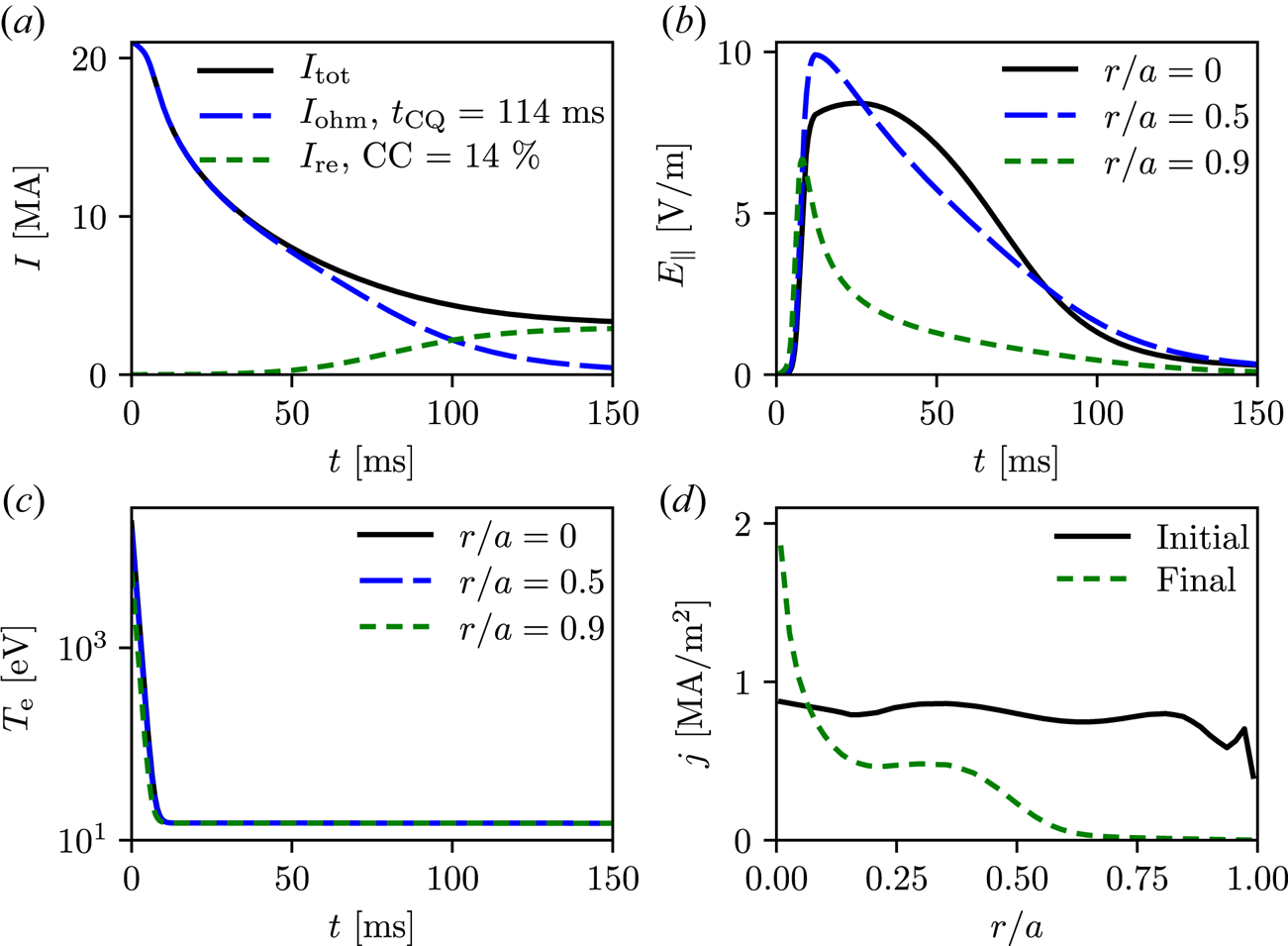
Figure 2. Plasma current, electric field and temperature evolution in the baseline case where $t_0=1\,{\rm ms}$ and $T_f=15\,{\rm eV}$
 . (a) Total plasma current (solid) as function of time, together with the ohmic (long dashed) and runaway (short dashed) contributions. (b,c) Electric field and electron temperature evolution at different radii, given in the legend. (d) Initial and final radial current density profiles.
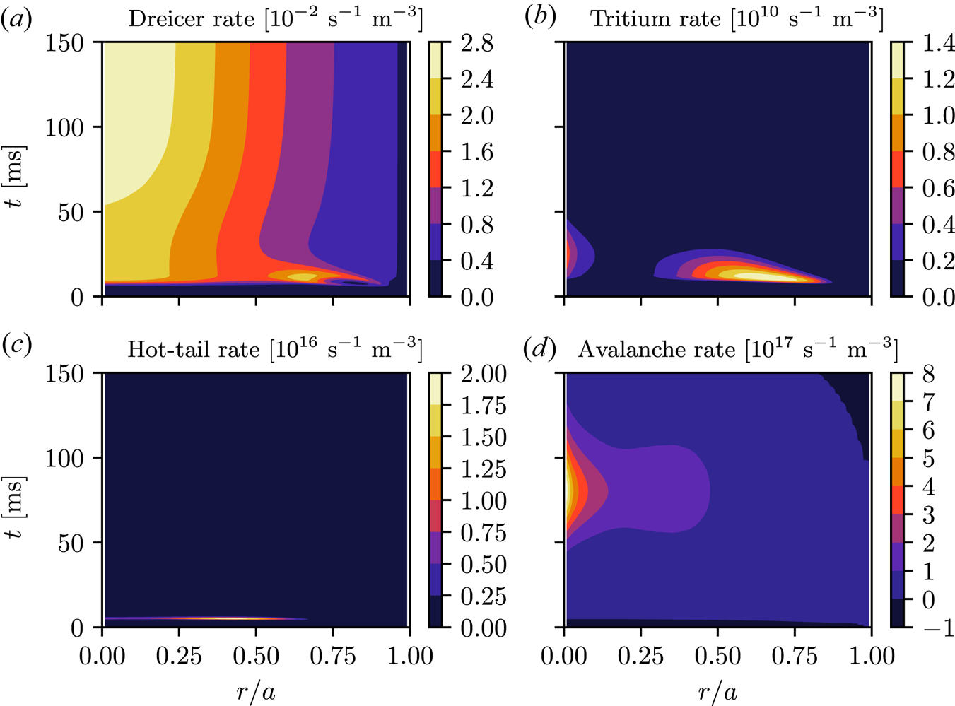
Figure 3. Time evolution of the radial distributions of the (a) Dreicer, (b) tritium decay, (c) hot-tail and (d) avalanche runaway rates, in the baseline case where $t_0=1\,{\rm ms}$ and $T_f=15\,{\rm eV}$
 . Note the different scales indicated in the panel headings.
The current conversion with this modest TQ time (Riccardo et al. Reference Riccardo and Loarte2005) is 14 %, meaning that this disruption would not be tolerable without mitigation due to the large runaway current generated. Figure 2(b) shows that the maximum of the electric field is approximately $10\,{\rm V}\,{\rm m}^{-1}$ , which is not sufficient to make the Dreicer contribution to the runaway generation significant, as is evident from figure 3(a). The runaway production is the largest on axis but also makes contributions for larger radii, as shown in figure 2(d). This differs from similar results for tokamaks with a more conventional shape, where the production only has the on-axis peak and approximately exponentially drops to zero for larger radii (Fülöp et al. Reference Fülöp, Helander, Vallhagen, Embreus, Hesslow, Svensson, Creely, Howard and Rodriguez-Fernandez2020).
In figure 3(c) we see that the dominant primary generation mechanism is the hot-tail, as its maximum value is approximately six orders of magnitude larger than that of the second most important mechanism, the tritium decay shown in figure 3(b). As the hot-tail generation happens very early during the disruption, where transport may be strong due to a high level of magnetic fluctuations, this result is likely to overestimate the hot-tail seed at the end of the TQ because transport has not been taken into account. When completely disabling the hot-tail seed, but otherwise using identical settings, the runaway conversion plummets to 0.0001 %, see table 1, thus 14 % can be taken as an upper limit for the current conversion in this case. Note, however, that $t_{\text {CQ}}$ is longer in the case where hot-tail generation is excluded and the CQ is incomplete after 150 ms, with approximately 2.1 MA ohmic current remaining. The residual ohmic current could potentially convert to runaway current beyond this point. However, when running this simulation for twice as long, i.e. until 300 ms, the resulting current conversion is instead 0.0005 %. This means that the runaway current is approximately 0.1 kA, still well below the limit, and the remaining ohmic current is approximately 0.3 MA – so if the entire hot-tail seed is lost through radial transport this is a disruption where mitigation would not be necessary.Footnote 2
Table 1. Current conversion, CQ time $t_{\text {CQ}}$ and remaining ohmic current at the end of the simulation (150 ms) for cases differing from the baseline case in one input parameter, as listed in the first column.

The overall dominant runaway mechanism is avalanche multiplication, with a maximum value of approximately two orders of magnitude larger than the hot-tail maximum, and with high rates for a much longer period of time, as seen in figure 3(d). As the avalanche gain increases exponentially with the initial plasma current, it is no surprise that avalanche is the dominant runaway generation mechanism in this case, where there is a high runaway seed and initial plasma current. Due to the dominance of the avalanche, the total runaway generation rate is almost identical to the avalanche rate and is therefore not shown separately. Also, it can be noted that there is a region with negative avalanche multiplication, which occurs when the electric field goes below the critical electric field (Hesslow et al. Reference Hesslow, Embréus, Wilkie, Papp and Fülöp2018b). A runaway electron can then lose enough energy when colliding with the thermal electron bulk that it falls out of the runaway region, without knocking the thermal electrons into the runaway region, and so the runaway density decreases in time.
3.3. Sensitivity study
In table 1 we summarise the current conversion factor, the CQ time and the remaining ohmic current for a number of different cases, including the baseline (entry at the top). The observed long CQ times (typically $t_{\rm CQ}>100\,{\rm ms}$ ) are due to the relatively high assumed post-TQ temperature, $15\,{\rm eV}$
 , which is consistent with the lack of impurity injection. As expected, the influence of tritium decay on the runaway rate is weak, as evident from table 1; neither the current conversion nor the CQ time is affected when changing the initial tritium content in the plasma between the two limiting cases of pure deuterium and pure tritium.
The plasma shape will in reality evolve during a disruption, so we compare the runaway generation in the highly shaped baseline configuration with a case with no shaping, i.e. a fixed circular cross-section with no Shafranov shift (the $j_0$ profile shown in figure 7(a) is then multiplied by 3 to keep the total current constant, neglecting the impact on plasma stability), to gain an understanding of the impact that shaping can have on the disruption dynamics. The trapping corrections on the generation rates are excluded in one of the variations, as trapping is expected to be strong in highly shaped compact tokamaks, when compared with conventional tokamaks. We find that, in both the case where trapping effects on the runaway generation mechanisms are excluded (no trapping), as well as the case with a circular cross-section (no shaping), the current conversion is increased and the CQ time is decreased. The physical reasons behind these changes are different in the two cases. In figure 4(a,b) the electric field and the current density profiles of these two cases are shown, together with the baseline case for comparison. The maximum electric field is notably higher in the no shaping case, which leads to the increased current conversion, as was seen also in Fülöp et al. (Reference Fülöp, Helander, Vallhagen, Embreus, Hesslow, Svensson, Creely, Howard and Rodriguez-Fernandez2020) for a conventional aspect ratio. In the no trapping case, the maximum electric field is the same but the current contributions at larger radii – where a significant fraction of particles can be trapped in a ST geometry – are increased, as seen in the radial distribution of the final current density.

Figure 4. Electric field evolution at $r/a=0.5$ (a,c) and final current densities (b,d). Panels (a,b) compare the baseline (solid) with the no shaping (long dashed) and no trapping (short dashed) cases. Panels (c,d) compare the baseline ($r_{\text {wall}}=0\,{\rm cm}$
 , $t_{\text {wall}}=\infty$
 , solid) with the cases using $r_{\text {wall}}=30\,{\rm cm}$
 (long dashed) and $t_{\text {wall}}=10\,{\rm ms}$
 (short dashed). In (b,d) the initial current density profile is also included (dotted).
We have also investigated the effects of changing the wall distance $r_\text {wall}$ and the wall time $t_\text {wall}$
 . The magnetic fields in conducting structures have a complex response to a disruption, which depends on the geometry and material composition, and this response is currently determined by the two numbers in dream, $r_\text {wall}$
 and $t_\text {wall}$
 . They can be estimated from measurements or detailed electromagnetic calculations, but, due to the uncertainty in these values for a preliminary reactor design like BurST, it is useful to let $r_\text {wall}$
 and $t_\text {wall}$
 vary, to understand the sensitivity of the result to the assumed values.
By increasing the wall distance from zero to $10\,{\rm cm}$ then to $30\,{\rm cm}$
 , or reducing the wall time from that of a perfectly conducting wall ($t_{\text {wall}}=\infty$
 ) to an ITER-like value $t_{\text {wall}}=0.5\,{\rm s}$
 and an even shorter value of $10\,{\rm ms}$
 , we find an increased current conversion, as well as increased $t_{\text {CQ}}$
 . The electric field and the current density for these cases can be seen in figure 4(c,d). In both cases the off-axis contributions are increased compared with the baseline; in the $r_{\text {wall}}>0$
 case this is due to magnetic energy returning to the plasma from the vacuum region between the plasma and the wall, while in the $t_{\text {wall}}<\infty$
 case it is magnetic energy from the wall and potentially the surrounding structures that diffuses back into the plasma. The stronger electric fields near the edge affect the generation mechanisms, such that more runaway production happens further away from the centre of the plasma. This is visible in the final current densities, which have a larger off-axis contribution. Another interesting observation concerning changing to a finite wall time is that the dynamics of the total current changes as a result of magnetic energy returning to the plasma from the wall. The effect of this is that a runaway plateau phase is not immediately reached after the CQ, but there is rather a long gradual increase in the runaway current before the plateau is reached, see figure 5(a). The time needed to reach the plateau in this case is much longer than $150\,{\rm ms}$
 , which is the time scale where the control over the plasma is deemed lost after a disruption. This implies that the maximum runaway current would depend strongly on when the control over the plasma is lost, as compared with the case of a perfectly conducting wall. Concerning runaway conversion, a tightly placed highly conducting wall is the most favourable choice, reducing the poloidal field energy diffusion back into the plasma and, as such, the accompanying avalanche gain.
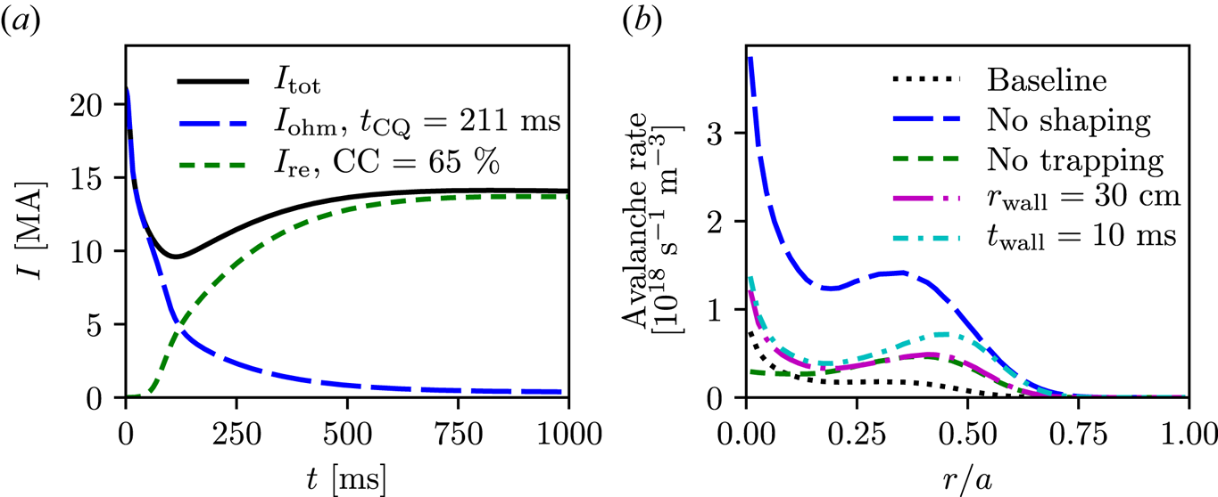
Figure 5. (a) Total plasma current (solid) as a function of time, together with the ohmic (long dashed) and runaway (short dashed) contributions, when using a finite wall time $t_{\text {wall}}=500\,{\rm ms}$ . Note the long time scale plotted, and compare with figure 2(a). (b) Characteristic radial profiles of the avalanche runaway rate: baseline case (dotted, see figure 2d), no shaping case (long dashed), no trapping case (short dashed), $r_{\text {wall}}=30\,{\rm cm}$
 case (long dash-dotted) and $t_{\text {wall}}=10\,{\rm ms}$
 case (short dash-dotted).
The final column of table 1 indicates the remaining ohmic current at the end of the simulations. Values of more than tens of kiloamperes indicate an incomplete CQ and we see that this is the situation in all variations evaluated. As noted above, the remaining ohmic current could become a problem, because it might be converted to runaway current if control over the plasma is lost at some later time. The case with the most residual ohmic current is that with a wall time of 500 ms (almost 9 times that in the baseline) and the case with the least is the no shaping case (approximately 6 times lower than that in the baseline case). This indicates that the strong ST shaping makes the residual ohmic current problem worse, whilst it reduces the initial runaway problem. Equilibria at conventional and tight aspect ratio, with attempts to match the current and plasma profiles, would be needed for a detailed understanding of the effect of aspect ratio, but such a study is beyond the scope of the present work.
Regarding the different generation mechanisms, we have already touched upon the weak influence of the tritium seed, as confirmed by the cases where the amount of tritium is varied. In all other cases tritium generation remains of the same order of magnitude. When and where the tritium runaway generation happens do, however, change, an example being the radial gap at around $r/a \approx 0.25$ in figure 3(b) disappearing in the no shaping and no trapping cases. In all cases in table 1 hot-tail is the dominant primary generation mechanism, whereas most of the runaway current is generated through the avalanche. As the parameters are varied, the only case which produces a change in the hot-tail generation compared with figure 3(c) is the no shaping case, where the electric field is stronger. In this case the hot-tail generation happens in the same radial range during the same time period, but the maximum value is increased by a factor of around five. As the avalanche multiplication dominates in all studied cases, it determines the shape of the final current density, which can be seen by comparing the profile of the avalanche rates for the parameter variations studied, as shown in figure 5(b), with the final current profiles in figure 4(b,d).
Finally, we considered the unmitigated evolution for BurST profiles which were not optimised for energy confinement (dotted lines in figure 7a–c). With other parameters taken to be the same as the baseline case, the current conversion increased to 22 %, compared with 14 % in the baseline case. This means that the profiles optimised for energy confinement also reduce the runaway production. We repeated the study of the effect of the parameter variations listed in table 1 for these un-optimised profiles and found the same trends in the runaway current conversion; the runaway current conversion stays the same or increases. This indicates that there is a robustness in the obtained results with respect to changes of this type in the input profiles.
4. Mitigation with massive material injection
In the previous section we found that reactor-scale ST disruptions can be expected to generate significant runaway populations, not atypical of disruptions in conventional reactor-scale tokamaks (Vallhagen et al. Reference Vallhagen, Embreus, Pusztai, Hesslow and Fülöp2020). Therefore, in this section we undertake a first study of the effectiveness of straightforward material injection mitigation on the runaway dynamics. The considered mitigation strategy is injection of a large quantity of mixed deuterium and neon. There are different schemes for injecting material into the plasma during a disruption. In the massive gas injection scheme neutral gas is released into the plasma through a valve in the tokamak wall (Hollmann et al. Reference Hollmann, Aleynikov, Fülöp, Humphreys, Izzo, Lehnen, Lukash, Papp, Pautasso and Saint-Laurent2015). Despite its relative simplicity, this method has a disadvantage: the material begins to ionise at the edge of the plasma as soon as it is injected, thus becoming magnetically confined before reaching and cooling the hottest central parts of the plasma. This issue is overcome in the shattered pellet injection (SPI) scheme – the baseline disruption mitigation technique in ITER (Lehnen et al. Reference Lehnen, Jachmich and Kruezi2020) – where frozen pellet shards are injected into the plasma. Here, the details of the material delivery are not considered and we work from assumed deposited material profiles. This also facilitates comparison of the results with material injection disruption mitigation effects studied previously in conventionally shaped tokamaks.
Due to the transport event of the TQ, the ion content in the plasma tends to undergo radial mixing, yielding a relatively homogeneous impurity content (Linder et al. Reference Linder, Fable, Jenko, Papp and Pautasso2020; Hu et al. Reference Hu, Nardon, Hoelzl, Wieschollek, Lehnen, Huijsmans, van Vugt and Kim2021). After the mixing, if the radial variation of impurities is not too strong, the final runaway current is usually not strongly modified compared with the case of homogeneous impurity density with the same total impurity content, as noted by Vallhagen et al. (Reference Vallhagen, Embreus, Pusztai, Hesslow and Fülöp2020). However, an edge localised impurity content can help by reducing the transported fraction of heat, as reported by Bergström & Halldestam (Reference Bergström and Halldestam2022). Here, we do not resolve this dynamics, rather assume the injected material to be uniformly deposited as neutrals at the start of the simulation.
In the material injection simulations the electron temperature is evolved self-consistently – according to equation (43) of Hoppe et al. (Reference Hoppe, Embreus and Fülöp2021) – during the entire simulation (ion temperatures are not evolved separately.Footnote 3) For the electron heat diffusion the magnetic perturbation amplitude $\delta B/B$ is estimated from the values for $t_0$
 and $T_f$
 during the TQ, such that the decay time scale before the radiative collapse is approximately $t_0$
 . The transport is active during the time it would take for the temperature to decay exponentially from the initial temperature to 100 eV, according to (2.4), after which the transport-induced losses represented by this perturbation generally no longer dominate. The estimate for the time over which this is active is conservative, as dilution, ionisation and radiation losses generally make the total TQ time shorter than this. Also, in reality, the flux surfaces tend to re-heal after the plasma has lost most of its thermal energy (Sommariva et al. Reference Sommariva, Nardon, Beyer, Hoelzl and Huijsmans2018), so the electron heat diffusivity drops rapidly. Our conservative estimate ensures that the transport is active here during the entire TQ. Having significant heat diffusivity after the plasma has reached a low quasi-equilibrium temperature has in fact very little effect, as then radiative heat losses dominate by a large factor.
Trapping corrections to the growth rates are turned off for the material injection simulations, as these effects are negligible at high densities and in the presence of significant impurity content, due to the high collisionality. Also note that trapping is less important in the presence of very high electric fields, as particles can be accelerated out from the trapped region faster than their orbit time (McDevitt & Tang Reference McDevitt and Tang2019). The same assumption was made by Vallhagen et al. (Reference Vallhagen, Embreus, Pusztai, Hesslow and Fülöp2020) when modelling mitigation in ITER-like plasmas.
We identify trends in the impact of material mitigation by scanning the injected deuterium and neon densities over the rangesFootnote 4 $n_{{D}}=10^{20}\,{\rm m}^{-3}\unicode{x2013}10^{22}\,{\rm m}^{-3}$ and $n_{\text {Ne}}=10^{16}\,{{\rm m}^{-3}}\unicode{x2013}10^{20}\,{{\rm m}^{-3}}$
 , which are similar to those previously used by Vallhagen et al. (Reference Vallhagen, Embreus, Pusztai, Hesslow and Fülöp2020). We consider mitigation of two cases, a high transport case with $\delta {B}/B\approx 0.6\,\%$
 representative of a fast TQ ($t_0= 1\,{\rm ms}$
 , $T_f= 10\,{\rm eV}$
 ) and a low transport case with $\delta {B}/B\approx 0.2\,\%$
 representative of a slow TQ ($t_0= 10\,{\rm ms}$
 , $T_f= 10\,{\rm eV}$
 ). Once the essential behaviour in these regimes is understood, the requirements to mitigate potential faster TQs should be the subject of more detailed future studies. The magnetic perturbations determining the transport were estimated based on the temperature decay parameters. With $t_0= 1\,{\rm ms}$
 , $T_f= 10\,{\rm eV}$
 the corresponding unmitigated case has a current conversion of 46 %, or equivalently a maximum runaway current of 9.7 MA, and $t_{\text {CQ}} = 75\,{\rm ms}$
 . Therefore, the mitigation objective in this case is to reduce the runaway current while keeping the CQ time within the limits. With $t_0= 10\,{\rm ms}$
 , $T_f= 10\,{\rm eV}$
 the corresponding unmitigated case has a vanishingly small current conversion, but an incomplete CQ with an ohmic current of 8.7 MA remaining at the end of the simulation. The goal of mitigation in this case is thus instead to make the ohmic current decay faster to obtain $t_{\text {CQ}}$
 between the limits, while keeping the runaway current at a low level.
The resulting maximum runaway current as a function of injected deuterium and neon is shown in figure 6(a,c) for the case with high transport and in figure 6(b,d) for the case with low transport. In figure 6(a,b) we show the result only accounting for diffusive heat transport due to the magnetic perturbations, whilst figure 6(c,d) also include the consistent diffusive radial transport of runaways – this can be seen to have a significant impact on the operating space. In these simulations the magnetic perturbations were applied only during the time it took for the temperature in the equivalent cases in figure 6(a,b) to fall to 100 eV, and are therefore less conservative. The figures include several boundaries for reference: lower $t_{\text {CQ}}$ boundary of 20 ms (short dashed, producing no constraint in figure 6d), two possible upper $t_{\text {CQ}}$
 boundaries of 100 ms (long dashed) and 150 ms (solid) as well as a boundary indicating 10 % of the thermal energy being lost through radial transport (short dash-dotted). As can be seen in all cases, there is a region of low runaway current (below 0.5 MA) for low injected densities, as well as at high neon and low deuterium density injected in the low transport case. In these regions of low runaway current the ohmic CQ is incomplete. This is evident from the regions being below or to the left of the solid lines, indicating that the injected deuterium–neon mixture is insufficient to induce a complete radiative collapse.

Figure 6. Maximum runaway current $I_{\text {re}}$ as a function of injected deuterium ($n_{{D}}$
 ) and neon ($n_{\text {Ne}}$
 ) densities, in the cases where (a,c) $\delta {B}/B\approx 0.6\,\%$
 and (b,d) $\delta {B}/B\approx 0.2\,\%$
 . Panels (a,b) include only heat transport whereas panels (c,d) include runaway transport as well. Between the short- and long-dashed lines, $t_{\text {CQ}}$
 takes values between 20 ms and 100 ms. To the left of the solid line, $t_{\text {CQ}}$
 is longer than 150 ms or the CQ is incomplete (in which case the CQ time would be much longer than 150 ms). Above the dash-dotted line the transported fraction of the thermal energy loss is lower than 10 %.
In figure 6(a,b), i.e. neglecting particle loss due to the magnetic perturbations, we see that in the region between the lower $t_{\text {CQ}}$ limit of 20 ms and the upper $t_{\text {CQ}}$
 limit of 100 ms runaway currents between 2.5 and 18 MA are obtained. If the upper CQ time limit can be extended to 150 ms, the region contains runaway currents down to 0 MA, around injected densities of $n_{{D}}\approx 1.6\times 10^{21}\,{{\rm m}^{-3}}$
 and $n_{\text {Ne}}\approx 1.5\times 10^{18}\,{{\rm m}^{-3}}$
 . However, we caution that the largest increase in the avalanche multiplication is here observed at the very end of the simulation. This is in accordance with Hesslow et al. (Reference Hesslow, Embréus, Vallhagen and Fülöp2019a), where the runaway generation is first suppressed by material injection, to later become large due to a stronger avalanche in the presence of heavy impurities. There is also approximately 1.4 MA ohmic current left, which thus could readily be converted to a runaway current if the plasma survived beyond the 150 ms mark.
We look in more detail at the region in figure 6(a) where the best performance in terms of low runaway current is obtained, that is $n_{{D}}\approx 1.6\times 10^{21}\,{{\rm m}^{-3}}$ and $n_{\text {Ne}}\approx 1.5\times 10^{18}\,{{\rm m}^{-3}}$
 , and find that the tritium, hot-tail and avalanche generation all behave differently to the corresponding unmitigated case. Hot-tail is still the dominant primary seed, although the maximum generation rate is reduced from ${\sim }10^{16}$
 to ${\sim }10^{7}\,\,{\rm s}^{-1}\,{\rm m}^{-3}$
 . Also, the generation only occurs over approximately 0.5 ms, compared with 2 ms in the unmitigated case, and is localised inside a more limited radial range around the plasma centre (up to $r/a\approx 0.6$
 rather than $r/a\approx 1.0$
 ). With this combination of injected deuterium–neon densities the fast electrons that formed the hot-tail in the unmitigated case slow down more before the electric field rises, leading to a smaller ‘tail’ that can be converted to runaways. The tritium seed is fully suppressed, which indicates that the critical runaway energy for generation through tritium decay is increased for this level of impurity injection, in accordance with results by Vallhagen et al. (Reference Vallhagen, Embreus, Pusztai, Hesslow and Fülöp2020). The smaller runaway seed currents lower the outcome of the avalanche multiplication, leading to the observed low runaway current.
When we now include particle loss due to the magnetic perturbations, see figure 6(c,d), a significant region opens up with both tolerable ohmic current evolution and runaway current. In the case of the fast TQ, where mitigation is needed to reduce the runaway current while keeping the CQ time within acceptable limits (figure 6c), this region occurs for $n_{{D}}$ above around $4\times 10^{21}\,{{\rm m}^{-3}}$
 and $n_{\text {Ne}}$
 in the range $1\unicode{x2013}20 \times 10^{18}\,{{\rm m}^{-3}}$
 . In the case of a slow TQ, where mitigation is needed to reduce the CQ time while keeping the runaway current low (figure 6d), this region appears for $n_{{D}} \approx 1.5\unicode{x2013}3.5\times 10^{21}\,{{\rm m}^{-3}}$
 with $n_{\text {Ne}} \approx 2 - 15 \times 10^{18}\,{{\rm m}^{-3}}$
 , then widens for $n_{{D}}$
 above $3.5\times 10^{21}\,{{\rm m}^{-3}}$
 to include $n_{\text {Ne}} \approx 1\unicode{x2013}40 \times 10^{18}\,{{\rm m}^{-3}}$
 . In these regions, the runaway currents range from 0 to approximately 1.5 MA. Looking again in detail at the point in figure 6(c) with $n_{{D}}\approx 1.6\times 10^{21}\,{{\rm m}^{-3}}$
 and $n_{\text {Ne}}\approx 1.5\times 10^{18}\,{{\rm m}^{-3}}$
 , we find that inclusion of the particle transport has reduced the maximum hot-tail generation rate to ${\sim }10^{5}\,\,{\rm s}^{-1}\,{\rm m}^{-3}$
 . This results in a weaker avalanche and the low runaway currents in this region. This process is responsible for opening the whole region of acceptable evolution in figure 6(c,d).
Finally, we take the limit on transported thermal energy loss into account, as well as the $t_{\text {CQ}}$ limits. We see from figure 6(a,b) that without accounting for particle transport by the magnetic perturbations there is no region where it is possible to fulfil all three demands simultaneously. In the regions above the short dash-dotted line in these figures, where the transported fraction is below 10 %, the runaway current is at least 11 MA. Including the particle transport only moderately affects the energy loss boundary in the slow TQ case, but the reduced runaway current generation does offer acceptable parameter spaces at high injected levels of deuterium and neon. The reason behind the transported fraction reaching high levels seems to be the shape of the initial temperature and density profiles, see figure 7(b,c), as compared with those studied previously at a conventional aspect ratio. For example, in the case with the lower $\delta B/B$
 for $n_{{D}}\approx 1.6\times 10^{21}\,{{\rm m}^{-3}}$
 and $n_{\text {Ne}}\approx 8.1\times 10^{18}\,{{\rm m}^{-3}}$
 , the transported fraction is 61 %. If we instead change to a flat initial density of $n_{e0} =10^{20}\,{{\rm m}^{-3}}$
 , as in Vallhagen et al. (Reference Vallhagen, Embreus, Pusztai, Hesslow and Fülöp2020), the transported heat loss fraction is reduced to approximately 33 %. If also the temperature profile is changed to that of Vallhagen et al. (Reference Vallhagen, Embreus, Pusztai, Hesslow and Fülöp2020), i.e. $T_0(r) = 20\times [1-(r/a)^2]\,{\rm keV}$
 , the fraction is further reduced to 14 %, very close to the acceptable level.

Figure 7. Radial profiles for initial (a) current density, (b) electron density and (c) temperature, both for the baseline case and the profiles not optimised for energy confinement. (d) Shape of the input equilibrium flux surfaces. The dashed lines correspond to the unmodified equilibrium and the solid lines indicate the modified flux surfaces used in the simulations. The thicker red lines mark the outermost flux surface in each case.
5. Discussion and conclusions
We have shown that mitigation would typically be required to keep the runaway current below acceptable levels in reactor-scale STs, and that the runaway generation is comparable to that seen in conventional tokamak reactor scenarios. The dominant primary generation mechanism is the hot-tail, that reaches 6 (18) orders of magnitude higher values than the tritium decay (Dreicer) seed, and the avalanche gain is very high, as expected for a high-current tokamak.
Whilst dedicated equilibria are needed to determine in detail the impact of aspect ratio on the observed runaway dynamics, our simulations show that both removing the shaping and removing the trapping corrections increase the runaway current in unmitigated disruptions. When removing the shaping the increase was due to a higher electric field, while the increase when removing the trapping correction was due to more current contributing at larger radii. This may naively suggest that if the plasma evolves from its highly shaped initial state through to a smaller, more circular configuration as the outer layers of plasma are possibly lost during the disruption, the runaway generation would increase compared with the results given here at constant shape. It is likely more complicated, however, as then the current density would not increase in the plasma core in such a process, while the scraped off current may be re-induced at the boundary of the plasma with flux surfaces. Increasing the wall distance or decreasing the wall time also leads to an increased runaway current. In both cases this increase was due to an increased energy reservoir, either from the vacuum between the plasma and the wall, or from the surrounding structures.
Whilst successful control of the ohmic current evolution and runaway currents seems to be within reach in the case of disruption mitigation by mixed deuterium–neon injection, quantities at the higher end of the range explored are required to control the transported energy level, due to the peaked density and large temperature pedestal.
There are several aspects of our analysis that could be expanded on to move towards quantitative predictions of the runaway generation in ST-based fusion reactors. Importantly, the effect of Compton seed due to vessel activation has previously been found to have a significant effect on runaway generation in conventional tokamaks due to Compton scattering. This was demonstrated for example by Vallhagen et al. (Reference Vallhagen, Embreus, Pusztai, Hesslow and Fülöp2020), where adequate mitigation for ITER-like parameters could not be achieved with mixed material injection in the activated phase of operations. Such modelling requires the spectrum of $\gamma$ -photons emitted from the plasma-facing components. This information for ITER is provided by Martín-Solís et al. (Reference Martín-Solís, Loarte and Lehnen2017), but it remains to be determined for alternative reactor designs. However, the runaway current in high-current devices is only a logarithmically weak function of the seed (Vallhagen et al. Reference Vallhagen, Embreus, Pusztai, Hesslow and Fülöp2020), so it might not have a major effect on the result, although it could have a more significant impact if the hot-tail and Dreicer seeds would be lost through transport during the TQ.
We have studied here the two limiting cases where either the same shaping was kept throughout the disruption or a circular cross-section was assumed throughout; dream does currently not allow for the evolution in time of the background magnetic geometry. A relatively straightforward generalisation yet to be implemented in the code would be to allow the shaping parameters of the analytical equilibrium model used here to evolve in time according to user-prescribed functions.
Regarding the material injection, it could be interesting to study another impurity, such as argon. Using a heavier impurity might lead to more radiation and thus possibly reduce the high transported fraction of the thermal energy loss, but at the same time we expect that it has the potential to lead to a larger avalanche, due to the larger number of bound target electrons (Hesslow et al. Reference Hesslow, Embréus, Vallhagen and Fülöp2019a). Also, relaxing the assumption of a flat density profile for the injected material would improve the model, as in reality the material is injected at the wall and in most cases begins to ionise immediately (Svenningsson et al. Reference Svenningsson, Embreus, Hoppe, Newton and Fülöp2021). Additionally, SPI might be considered instead of assuming uniform material deposition at $t=0$ , as this would allow study of the impact of parameters related to SPI (e.g. pellet velocity, number of shards) on runaway conversion.
Finally, we have employed spatially homogeneous prescribed diffusivities. The possible richness of the spatio-temporal dynamics of transport coefficients, including instability onsets, partial stochastisation of the magnetic field (Pusztai et al. Reference Pusztai, Hoppe and Vallhagen2022) and flux surface re-formation (Izzo et al. Reference Izzo, Pusztai, Särkimäki, Sundström, Garnier, Weisberg, Tinguely, Paz-Soldan, Granetz and Sweeney2022), is not captured here. However, these aspects are known to have significant impact on the runaway current evolution, thereby presenting a major uncertainty in our predictions. As a fully self-consistent modelling of the three-dimensional processes at play implies many orders of magnitude larger computational requirements, exploration of the parameter space is bound to rely on reduced models. Distilling the results of three-dimensional simulations to simple models with respect to instability onset criteria, scalings of magnetic perturbation amplitudes and their spatial structure, as well as models for the flux surface re-formation dynamics, would indeed represent a major advance in the predictive power of reduced models, such as the one employed here.
Acknowledgements
The authors are grateful to T. Hender, B. Patel, H. Bergström, P. Halldestam, L.-G. Eriksson and E. Nardon for fruitful discussions.
Editor Per Helander thanks the referees for their advice in evaluating this article.
Funding
This work was supported by the Swedish Research Council (Dnr. 2018-03911) and part funded by the EPSRC Energy Programme [grant number EP/W006839/1] and the Swiss National Science Foundation. The work has been carried out within the framework of the EUROfusion Consortium, funded by the European Union via the Euratom Research and Training Programme (Grant Agreement No 101052200 – EUROfusion). Views and opinions expressed are, however, those of the author(s) only and do not necessarily reflect those of the European Union or the European Commission. Neither the European Union nor the European Commission can be held responsible for them.
Declaration of interests
The authors report no conflict of interest.
Appendix. Details of the input parameters
The BurST profiles for the initial total current density, electron density and temperature used in our simulations are shown in figure 7(a–c) (Patel Reference Patel2021). The total initial plasma current is $I_{\text {tot},0}=21\,{\rm MA}$ . Solid lines show the baseline profiles, which were obtained by optimising the energy confinement with respect to microinstabilities in BurST. An example of un-optimised profiles, shown as dotted lines in figure 7(a–c), are used here to study the impact of changes in the input profiles on the results. In figure 7(d) the flux surfaces of the input equilibrium are shown. The plasma major and minor radii are $R_0=3.05\,{\rm m}$
 and $a=1.5\,{\rm m}$
 , respectively, and the elongation at the outermost flux surface is $\kappa (a)=2.8$
 .
.
In a ST the poloidal and toroidal magnetic field components can be comparable, so the magnetic field strength may have more than one minimum on a flux surface (Wilson et al. Reference Wilson, Ahn, Akers, Applegate, Cairns, Christiansen, Connor, Counsell, Dnestrovskij and Dorland2004), which is the case here. As this is incompatible with the requirements on the input by dream, in our simulations the shaping profiles have been slightly modified to avoid multiple magnetic field minima. The double magnetic field strength minima on the outer flux surfaces are caused by the large Shafranov shift, $\Delta$ , which is approximately $-0.5\,{\rm m}$
 at the edge. We empirically found that limiting the edge value of the Shafranov shift to $-0.3\,{\rm m}$
 is sufficient to avoid the issue of double minima. Therefore we modified the slope of the Shafranov shift profile for large $r$
 to obtain $\Delta (r=a)\approx -0.3\,{\rm m}$
 . As we keep $R_0$
 fixed, this implies a shift of the outermost flux surface, since $\Delta (r=0)=0$
 according to the definition of the Shafranov shift in dream. The flux surfaces of the unmodified equilibrium are shown as dashed lines. By running simulations for varying radial location of the outermost flux surface, we confirmed that the sensitivity of the results to the shift is negligible.


 Open access