


1. Introduction
Gravity currents are flows driven by a density difference and occur ubiquitously in geophysical environments, including see-breeze fronts, pyroclastic flows, powder-snow avalanches and turbidity currents (Simpson Reference Simpson1997) and in man-made environments such as the accidental release of dense industrial gases (Fannelop Reference Fannelop1994). At the leading edge of the gravity currents, the characteristic morphological features in a three-dimensional view are the lobes and clefts. The lobes are described as projecting noses with bulges or buttresses which continually change shape and the clefts are described as deep indentations which divide the lobes along the front (Simpson Reference Simpson1972). The existence of lobes and clefts at the leading edge of the gravity currents is known to have implications for the frontal mixing in gravity currents (Simpson Reference Simpson1982), erosional and depositional patterns in turbidity currents (Allen Reference Allen1971, Reference Allen1985; Espath et al. Reference Espath, Pinto, Laizet and Silvestrini2015) and the dynamics of powder-snow avalanches (Jackson, Turnbull & Munro Reference Jackson, Turnbull and Munro2013).
Our understanding of the lobe-and-cleft structure at the leading edge of the gravity currents is largely based on laboratory experiments (e.g. Simpson Reference Simpson1972; Cenedese & Adduce Reference Cenedese and Adduce2008; La Rocca et al. Reference La Rocca, Adduce, Sciortino and Pinzon2008; Adduce, Sciortino & Proietti Reference Adduce, Sciortino and Proietti2012) and numerical simulations (e.g. Daly & Pracht Reference Daly and Pracht1968; Härtel, Meiburg & Necker Reference Härtel, Meiburg and Necker2000b; Cantero et al. Reference Cantero, Lee, Balachandar and Garcia2007b, Reference Cantero, Balachandar, Garcia and Bock2008; Ottolenghi et al. Reference Ottolenghi, Prestininzi, Montessori, Adduce and La Rocca2018) of gravity currents in a lock-exchange configuration. It is generally accepted that, based on laboratory experiments and numerical simulations, the generation of the lobe-and-cleft structure requires a no-slip boundary and the lobe-and-cleft structure is suppressed with a free-slip boundary (Simpson Reference Simpson1972; Britter & Simpson Reference Britter and Simpson1978; Härtel et al. Reference Härtel, Meiburg and Necker2000b; Xie, Tao & Zhang Reference Xie, Tao and Zhang2019). Due to the presence of a no-slip boundary, the lowest streamlines in the flow relative to the head must be towards the rear and the foremost point of a bottom-propagating gravity current head must be raised some distance above the bottom boundary. In a translating coordinate system which moves with the gravity current head, the stagnation point is located below and slightly behind the foremost point in the vicinity of the wall (Härtel et al. Reference Härtel, Meiburg and Necker2000b). This feature of the flow topology gives rise to an unstably stratified region between the stagnation point and the foremost point (Hartel, Carlsson & Thunblom Reference Hartel, Carlsson and Thunblom2000a) and the mechanism that leads to the initial formation of the lobe-and-cleft structure is shown to be the Rayleigh–Taylor instability (Xie et al. Reference Xie, Tao and Zhang2019). The characteristic initial lobe width based on the linear stability analysis has been found to agree with the lobe width based on three-dimensional direct numerical simulations of the initial formation of the lobe-and-cleft structure (Hartel et al. Reference Hartel, Carlsson and Thunblom2000a; Xie et al. Reference Xie, Tao and Zhang2019).
Once the lobes and clefts form at the leading edge of the gravity currents, the lobes move laterally along the leading edge while continuing to grow, shrink or breakdown into smaller ones. The clefts may continually merge with neighbouring clefts while new clefts appear as the large lobes split into smaller ones. The merging of clefts and splitting of lobes in the lobe-and-cleft structure continue ceaselessly as the gravity currents propagate in the streamwise direction. We should remark that the characteristic initial lobe width based on linear stability analysis corresponds to the initial formation of the lobe-and-cleft structure. When the above merging and splitting processes are clearly recognized, the lobe width is notably greater than the initial lobe width and does not correspond to the linearly unstable mode (Xie et al. Reference Xie, Tao and Zhang2019).
When the merging and splitting processes are present, the experiments of Simpson (Reference Simpson1972) indicate the following empirical relationship for the lobe width
 \begin{equation} \frac{\tilde{b}}{\tilde{d}} = 7.4 Re^{{-}0.39 \pm 0.02}_f \quad \mbox{and} \quad \frac{\tilde{b}_{max}}{\tilde{d}} = 12.6 Re^{{-}0.38 \pm 0.02}_f,\end{equation}
where  $\tilde {b}$ is the overall mean lobe width, $\tilde {b}_{max}$ is the mean of the maximum lobe width and $\tilde {d}$ is the height of the gravity current head. Here, the front Reynolds number is defined as $Re_f = \tilde {u}_f \tilde {d} / \tilde {\nu }$, where $\tilde {u}_f$ is the front velocity and $\tilde {\nu }$ is the kinematic viscosity of fluid. The front Reynolds number in the experiments of Simpson (Reference Simpson1972) was in the range $3 \times 10^2 \le Re_f \le 10^4$.
In laboratory scale gravity currents, the lobe size is dependent on the Reynolds number, where the Reynolds number on the laboratory scale is typically in the range from  $O(10^2)$ to $O(10^4)$. In the geophysical scale gravity currents, the lobe size is between $\tilde {d}$ and $2 \tilde {d}$ (Lawson Reference Lawson1971; O'Donnell, Ackleson & Levine Reference O'Donnell, Ackleson and Levine2008; Mayor Reference Mayor2011; Warrick & Stevens Reference Warrick and Stevens2011; Horner-Devine & Chickadel Reference Horner-Devine and Chickadel2017) and there is no evidence of Reynolds number dependence, where the Reynolds number on the geophysical scale often exceeds $O(10^6)$. Horner-Devine & Chickadel (Reference Horner-Devine and Chickadel2017) speculate that the lobes and clefts in the geophysical scale gravity currents may result from the collapse of Kelvin–Helmholtz billows (Parsons Reference Parsons1998). More detailed field observations are still necessary to determine the lobe-and-cleft generation mechanism in the geophysical scale gravity currents (Horner-Devine & Chickadel Reference Horner-Devine and Chickadel2017) and the lobes and clefts in the geophysical scale gravity currents are not within the scope of this study.
Our aim in this study is to deepen the understanding of the vortical structure and the mechanism responsible for the merging of clefts and splitting of lobes for gravity currents propagating on the no-slip boundary. As we will show later, for the merging process, it requires the interaction of three tooth-like vortices and the middle tooth-like vortex breaks up and reconnects with the two neighbouring tooth-like vortices. For the splitting process, a new born streamwise vortex is created by the parent vortex of opposite orientation, attributed to the Brooke–Hanratty mechanism reinforced by the baroclinic production of vorticity, and the parent vortex can be either the left part or the right part of the existing tooth-like vortex inside the splitting lobe. To the best of our knowledge, even though the lobe width has been measured in experiments (Simpson Reference Simpson1972) for planar gravity currents and in numerical simulations (Cantero, Balachandar & Garcia Reference Cantero, Balachandar and Garcia2007a; Cantero et al. Reference Cantero, Lee, Balachandar and Garcia2007b) for cylindrical and planar gravity currents, there is no existing report in the literature that documents the evolution of the vortical structure inside the splitting lobe and the mechanism responsible for the splitting process. Our investigation is conducted by means of three-dimensional high-resolution simulations of the incompressible Navier–Stokes equations with the Boussinesq approximation. The problem is designed following the experiments of Simpson (Reference Simpson1972) in that the gravity currents are produced from a full-depth lock-exchange configuration and the lock length is sufficiently long such that the gravity currents are maintained in the slumping phase. In the slumping phase, the leading edge of the gravity currents travels at approximately constant speed and we may systematically vary the Reynolds number in the problem. The paper is organized as follows. In § 2, we describe the formulation of the problem. The qualitative and quantitative results are presented in § 3. Finally, conclusions are drawn in § 4.
2. Formulation
In the present work we focus on gravity currents in the slumping phase produced from a full-depth lock-exchange set-up with a no-slip boundary. Figure 1 sketches the initial condition for a full-depth lock-exchange flow. The height of the channel is  $\tilde {H}$ and the width of the channel is $\tilde {L}_{x_2}$. The length of the channel is $\tilde {L}_{x_1}$ while the length of the heavy fluid on the left side is $\tilde {L}_0$. The heavy fluid on the left side has density $\tilde {\rho }_1$ and the ambient fluid has density $\tilde {\rho }_0$. We assume that the density difference is sufficiently small, i.e. $(\tilde {\rho }_1-\tilde {\rho }_0) \ll \tilde {\rho }_0$, such that the Boussinesq approximation (the influence of density variations is retained only in the buoyancy term but neglected in the inertia and diffusion terms) can be adopted.

Figure 1. Sketch of the initial condition for a full-depth lock-exchange flow. The heavy fluid has density  $\tilde {\rho }_1$, height $\tilde {H}$ and length $\tilde {L}_0$. The ambient fluid of the same height has density $\tilde {\rho }_0$ and length $\tilde {L}_{x_1} - \tilde {L}_0$. The coordinate system follows the right-hand rule, where $x_1, x_2$ and $x_3$ represent the streamwise, spanwise and wall-normal directions, respectively. Here, the gravity $\tilde {g}$ acts in the negative $x_3$ direction and the positive spanwise direction points into the paper.
The governing equations under the Boussinesq approximation take the following dimensionless form
 $$\begin{gather} \frac{\partial u_{k}}{\partial x_k} = 0, \end{gather}$$
 $$\begin{gather}\frac{\partial {u}_{i}}{\partial t} + \frac{\partial ( {u}_{i} u_k ) }{\partial x_k} = \rho e^{g}_{i} - \frac{\partial p}{\partial x_i} + \frac{1}{Re} \frac{\partial^2 u_i }{\partial x_k \partial x_k}, \end{gather}$$
 $$\begin{gather}\frac{\partial {\rho}}{\partial t} + \frac{\partial ({\rho} u_k) }{\partial x_k} = \frac{1}{Re Sc} \frac{\partial^2 {\rho}}{ \partial x_k \partial x_k}, \end{gather}$$
where the dimensionless parameters in the governing equations are the Reynolds number  $Re$ and the Schmidt number $Sc$, defined by
 \begin{equation} Re = \frac{\tilde{u}_b \tilde{H}}{\tilde{\nu}} \quad \mbox{and} \quad Sc = \frac{\tilde{\nu}}{\tilde{\kappa}}, \end{equation}
respectively. The heavy fluid and ambient fluid are assumed to have identical kinematic viscosity  $\tilde {\nu }$ and molecular diffusivity $\tilde {\kappa }$ in the density field. Here, ${{u}_i}$ denotes the velocity, $\rho$ the density, ${{e}}^{g}_{i}=(0,0,-1)^{T}$ the unit vector in the direction of gravity and $p$ the pressure. The set of (2.1)–(2.3) is made dimensionless by the lock height, $\tilde {H}$, as the length scale, the buoyancy velocity
 \begin{equation} \tilde{u}_b=\sqrt{\tilde{g}'_0 \tilde{H}} \quad \mbox{with } \tilde{g}'_0 = \tilde{g} \frac{\tilde{\rho}_{1} - \tilde{\rho}_{0}}{\tilde{\rho}_{0}}, \end{equation}
as the velocity scale, where  $\tilde {g}$ is gravity, and $\tilde {H} \tilde {u}^{-1}_b$ as the time scale. The dimensionless density is given by
 \begin{equation} \rho = \frac{\tilde{\rho} - \tilde{\rho}_0}{\tilde{\rho}_1 - \tilde{\rho}_0}, \end{equation}
which varies in the range  $0 \le \rho \le 1$. Note that for the initial condition, $\rho =1$ represents the heavy fluid and $\rho =0$ represents the ambient fluid.
In all simulations discussed in this paper, we have used a Schmidt number of unity as setting the Schmidt number to unity is a common practice in simulations (Cantero et al. Reference Cantero, Balachandar and Garcia2007a,Reference Cantero, Lee, Balachandar and Garciab; Dai Reference Dai2015; Zgheib, Ooi & Balachandar Reference Zgheib, Ooi and Balachandar2016). Furthermore, it has been shown that the influence of the Schmidt number is weak as long as  $Sc \approx O(1)$ or larger (e.g. Härtel et al. Reference Härtel, Meiburg and Necker2000b; Necker et al. Reference Necker, Härtel, Kleiser and Meiburg2005; Bonometti & Balachandar Reference Bonometti and Balachandar2008). Since the gravity currents in the designed problem are maintained in the slumping phase during which the front travels at a constant speed $\tilde {u}_f$, we may define the dimensionless front speed in the slumping phase
 \begin{equation} Fr = \frac{\tilde{u}_f}{\tilde{u}_b},\end{equation}
as the Froude number. The front Reynolds number is defined as  $Re_f = \tilde {u}_f \tilde {d} / \tilde {\nu }$, which is related to $Re$ in (2.4a,b) and $Fr$ in (2.7) via
 \begin{equation} Re_f = \frac{\tilde{d}}{\tilde{H}} Re Fr.\end{equation}
 The governing equations in the velocity–pressure formulation is solved in the three-dimensional domain  $L_{x_1} \times L_{x_2} \times L_{x_3} = 17 \times 1.5 \times 1$, where the length of the heavy fluid is $L_0 = 8$ such that the slumping phase continues for extended spatial and temporal regions. Fourier expansion with periodic boundary condition is employed in the streamwise and spanwise directions. Chebyshev expansion with Gauss–Lobatto quadrature points is employed in the wall-normal direction. At the top and bottom walls, we employ no-slip condition for the velocity field and no-flux condition for the density field. The influence of the periodic boundary condition in the streamwise direction has been shown to be unimportant unless when the gravity currents have approached the boundary to within one length scale $\tilde {H}$ (Härtel et al. Reference Härtel, Meiburg and Necker2000b). Regarding the top boundary condition used in the simulation, our experiences in the laboratory experiments show that the feature of the lobe-and-cleft structure is persistent in the lock-exchange experiment irrespective of whether there is a lid or not on the top boundary. It was also shown in the numerical simulations by Cantero et al. (Reference Cantero, Lee, Balachandar and Garcia2007b) that with no-slip condition at the top and bottom walls, the direct numerical simulation results agree with the lock-exchange experiments. We should also remark that for the Boussinesq case as considered in this study and Cantero et al. (Reference Cantero, Lee, Balachandar and Garcia2007b), the influence of the density difference on the free surface is relatively small and the free surface can be assimilated to a top lid. For the non-Boussinesq case when the density difference is not small, the amplitude of the waves on the free surface may increase with the density difference and the experiments with a lid and without a lid may differ sensibly.
We adopt the low-storage third-order Runge–Kutta scheme (Williamson Reference Williamson1980) for time advancement. The convection and buoyancy terms are treated explicitly and the diffusion terms are treated with Crank–Nicolson scheme. For the convection term, divergence and convective forms are alternately used (Durran Reference Durran1999) and the  $3/2$-rule technique is adopted for the aliasing removal (Canuto et al. Reference Canuto, Hussaini, Quarteroni and Zang1988). This de-aliased pseudospectral code has been employed in Cantero et al. (Reference Cantero, Balachandar and Garcia2007a,Reference Cantero, Lee, Balachandar and Garciab) and Dai (Reference Dai2015) and Dai & Wu (Reference Dai and Wu2016) for lock-exchange flows. The initial velocity field was set with a quiescent condition in all simulations. The initial density field was prescribed as
 \begin{equation} \rho (x_1,x_2,x_3)|_{t=0} = \frac{1+\gamma_1}{2} ( 1 - \textrm{{erf}} \{ {\sqrt{Re Sc}} [ x_1 - ( L_0+\gamma_2 ) ] \}), \end{equation}
which is unity in the heavy fluid region and zero for the ambient fluid region with an error-function-type transition in the interface region, of which the thickness depends on the Reynolds number and Schmidt number. The values of  $\gamma _1$ and $\gamma _2$ were minute, uniform, random disturbances selected in the range $\gamma _1 \in (-0.05,0)$ and $\gamma _2 \in (-\Delta x_1/2, \Delta x_1/2)$ following Härtel, Michaud & Stein (Reference Härtel, Michaud and Stein1997) and Cantero et al. (Reference Cantero, Balachandar, Garcia and Ferry2006). In this study we are interested in the lobe-and-cleft structure and the merging and splitting processes within it. Therefore, the Reynolds number in the problem must be sufficiently high to support the initial formation and subsequent evolution of the lobe-and-cleft structure. We considered five Reynolds numbers, i.e. $Re=1788, 3450, 8950, 13000, 17000$, which correspond to the five front Reynolds numbers, i.e. $Re_f=383, 743, 1799, 2618, 3267$. To be consistent with the resolution requirement that the grid spacing must be of the order of $O{(Re Sc)}^{-1/2}$ (Härtel et al. Reference Härtel, Meiburg and Necker2000b; Birman, Martin & Meiburg Reference Birman, Martin and Meiburg2005), we employed the grid $N_{x_1} \times N_{x_2} \times N_{x_3}=616 \times 56 \times 88, 640 \times 84 \times 110, 1024 \times 112 \times 180, 1260 \times 140 \times 220, 1440 \times 160 \times 256$ in the three-dimensional simulations for the preceding five Reynolds numbers. The time step was chosen such that the Courant number remained less than $0.5$.
3. Results
3.1. Flow at the leading edge of the gravity currents
A typical appearance of the lobe-and-cleft structure at the leading edge of the gravity currents when the merging and splitting processes are at work is shown in figure 2. It is clear that the lobe-and-cleft structure is of a three-dimensional nature and lobes of different sizes coexist when the merging and splitting processes are at work. The experiments of Simpson (Reference Simpson1972), McElwaine & Patterson (Reference McElwaine and Patterson2004) and numerical simulations of Härtel et al. (Reference Härtel, Meiburg and Necker2000b) show that there exists a regular pattern of lobes with a preferred lobe width during the initial formation of the lobe-and-cleft structure. However, this regular pattern quickly evolves into a state where the merging and splitting processes are at work and lobes of different sizes may shift sideways along the advancing front. Furthermore, it was reported that the lobes may grow, shrink or breakdown and a cleft may continually merge with another neighbouring cleft.

Figure 2. Three-dimensional view of the lobes and clefts at the leading edge of a gravity current propagating on a no-slip boundary when the merging and splitting processes are at work. The Reynolds number in the simulation is  $Re=3450$ and the time instance is chosen at $t=5.66$ dimensionless units ( $\tilde {H} \tilde {u}^{-1}_b$). Flow field is visualized by a density isosurface of $\rho =0.2$. Side plane: instantaneous streamlines in a translating coordinate system. Bottom plane and back plane: density contours. Spacing between consecutive grid lines in the streamwise and spanwise directions is chosen at one-tenth of a dimensionless unit.
In the upper part of the head, the surface behind the clefts steepens. In the lower part of the head, the ambient fluid is diverted around the lobes and drawn into the clefts. Therefore, the bottom density contour shows an imprint of the lobe-and-cleft structure, where the heavy fluid advances in the lobe region and the ambient fluid is trapped in the cleft region. Due to the action of buoyancy, the ambient fluid trapped in the cleft region tends to rise in the head from the bottom boundary as shown by the mushroom-like shape in the cross-sectional density contour in the back plane of figure 2.
In order to unambiguously measure the height of the head, the height of the foremost point and the front location and to compare our results with the simulations of Härtel et al. (Reference Härtel, Meiburg and Necker2000b), here, we use the average in the spanwise direction for the dimensionless density and velocity in three-dimensional simulations. The average of a variable  $f(x_1,x_2,x_3)$ in the spanwise direction is defined as
 \begin{equation} \bar{f}(x_1, x_3) = \frac{1}{L_{x_2}} \int_0^{L_{x_2}} f(x_1, x_2, x_3) \, \textrm{d}\kern0.06em x_2, \end{equation}
where the variable  $f$ can be the dimensionless density $\rho (x_1, x_2, x_3)$ and velocity $u_i(x_1, x_2, x_3)$, where $i=1,2,3$ and $L_{x_2}=1.5$ is chosen in the three-dimensional simulations.
Figure 3 shows the spanwise-averaged flow field of the gravity current propagating on a no-slip boundary at  $Re=3450$ in the coordinate system moving with the head. The average of the spanwise velocity $\bar {u}_2$ is approximately zero. Consistent with the observations of Härtel et al. (Reference Härtel, Meiburg and Necker2000b), our spanwise-averaged flow field of the head is very similar to the corresponding two-dimensional flow field of the head.

Figure 3. Spanwise-averaged flow field of the gravity current on a no-slip boundary at  $Re=3450$ in the coordinate system moving with the head. The time instance is chosen at $t=5.66$ dimensionless units ( $\tilde {H} \tilde {u}^{-1}_b$). The thick solid line represents $\bar {\rho }=0.2$ and the velocity field ( $\bar {u}'_1,\bar {u}_3$) in the translating coordinate system is visualized by the thin solid streamlines. The stagnation point in the translating coordinate system is designated by the solid circle, of which the height is $x_{3s}$ above the bottom boundary, and the foremost point (nose) is designated by the solid square, of which the height is $x_{3n}$ above the bottom boundary.
In the translating coordinate system, we use a relative coordinate  $x'_1 = x_1 - x_f$ and a relative velocity $u'_1 = u_1 - u_f$, where $x_f$ and $u_f$ are the front location and front speed in the slumping phase, respectively. In the translating coordinate system moving at $u_f$, the head is stationary while the ambient fluid is approaching the head from the far end uniformly across the depth. In all cases considered in this study, the stagnation point, as shown in figure 3, is located below the foremost point of the head and the stagnation streamline close to the bottom boundary separates the ambient flow into two parts. While the oncoming ambient fluid above the stagnation streamline passes up and over the head, the oncoming ambient fluid below the stagnation streamline ends up being pulled underneath the head. Previously, only the thin layer of ambient fluid below the stagnation streamline was thought to flow into the clefts and the ratio of the amount of ambient flow $\dot {V}_u$ into the clefts to the total volume flux $\dot {V}_0$ can be estimated based on the height of the stagnation streamline at the far upstream end. Table 1 lists the fraction of the total volume flux that goes into the clefts based on the spanwise-averaged flow field as $\dot {V}_u/\dot {V}_0|_{2D}$ and shows that this fraction decreases as the Reynolds number increases from $1.51\,\%$ at $Re=1788$ ( $Re_f=383$) to $1.10\,\%$ at $Re=3450$ ( $Re_f=743$), $0.74\,\%$ at $Re=8950$ ( $Re_f=1799$), $0.61\,\%$ at $Re=13\ 000$ ( $Re_f=2619$) and $0.55\,\%$ at $Re=17000$ ( $Re_f=3267$). As a matter of fact, due to the three-dimensional nature of the lobe-and-cleft structure, not only the ambient fluid underneath the stagnation streamline can be diverted around the lobes and into the clefts but also the ambient fluid above the stagnation streamline, if not flowing into the clefts directly, can do likewise. Therefore, to estimate the fraction of the total volume flux going into the clefts in a three-dimensional lobe-and-cleft structure, $\dot {V}_u/\dot {V}_0|_{3D}$, we should consider that the ambient fluid which is ultimately trapped into the clefts may come from various upstream regions. To do this, we first calculate the ambient volume flux which passes up and over the head in the three-dimensional translating coordinate system. The ambient volume flux which goes into the clefts can then be calculated by subtracting the ambient volume flux which passes up and over the head from the total volume flux. The fraction of the total volume flux which goes into the clefts based on the three-dimensional lobe-and-cleft structure $\dot {V}_u/\dot {V}_0|_{3D}$, also listed in table 1, consistently decreases with increasing Reynolds number as $\dot {V}_u/\dot {V}_0|_{2D}$ demonstrates. However, quantitatively, the estimates based on the three-dimensional lobe-and-cleft structure $\dot {V}_u/\dot {V}_0|_{3D}$ are significantly greater than the corresponding estimates based on the spanwise-averaged two-dimensional flow field $\dot {V}_u/\dot {V}_0|_{2D}$.
Table 1. Quantitative information on the gravity current head in the slumping phase. The Reynolds number ( $Re$), front Reynolds number ( $Re_f$) and Froude number ( $Fr$) are defined by (2.4a,b), (2.8) and (2.7), respectively. The friction velocity ( $u^*$) in the gravity current head region is defined by (3.2a,b). The height of the foremost point (nose) above the bottom boundary is $x_{3n}$ and the height of the stagnation point is $x_{3s}$. The fraction of the total volume flux into the clefts based on the stagnation streamline in the spanwise-averaged flow field is $\dot {V}_u/\dot {V}_0|_{2D}$ and the fraction of the total volume flux into the clefts based on the three-dimensional lobe-and-cleft structure is $\dot {V}_u/\dot {V}_0|_{3D}$.

The evolution of the leading edge of the gravity current at  $Re=3450$ is shown as solid lines on the $(x_1,x_2)$ plane in figure 4. The leading edge is visualized by contours of $\rho =0.1$ close to the bottom boundary at $x_3=0.04$. The dashed lines are drawn to show the continuity of the clefts. The evolution of the lobes and clefts for other cases are qualitatively similar and therefore are not shown here. It can be seen that a cleft may continually merge with another neighbouring cleft and the lobes grow in size until they breakdown into smaller ones. The blue circle in figure 4 indicates the location of the merging, which will be discussed in § 3.2.1, and the red cross indicates the location of the splitting, which will be discussed in § 3.2.2. Following Simpson (Reference Simpson1972), the mean of the lobe width $\tilde {b}$ in figure 4 for the gravity currents in the slumping phase can be measured by counting the number of lobes in the spanwise direction and the mean of the maximum lobe width $\tilde {b}_{max}$ can be measured immediately before the splittings occur.

Figure 4. The evolution of the leading edge of the gravity current at  $Re=3450$ on the $(x_1,x_2)$ plane. The flow is from the left to right and the leading edge is visualized by contours of $\rho =0.1$ close to the bottom boundary at $x_3=0.04$ as solid lines. Time interval between consecutive contours is chosen at $\Delta t = 0.28$. The dashed lines show the continuity of the clefts. The blue colour $\bigcirc$ and red colour $\times$ indicate the locations where the merging process in § 3.2.1 and the splitting process in § 3.2.2 occur.
Figure 5 shows the mean of the lobe width and the mean of the maximum lobe width in the spanwise direction. The lobe width and the maximum lobe width are sampled following Simpson (Reference Simpson1972) for the mean values when the merging and splitting processes are at work and for a time span of approximately ten dimensionless time units. Our simulation results agree quantitatively with Simpson (Reference Simpson1972) and confirm the dependence of the lobe width on the front Reynolds number as indicated in (1.1a,b).

Figure 5. Ratio of the mean of the lobe width to the height of the gravity current head,  $\tilde {b}/\tilde {d}$, and ratio of the mean of the maximum lobe width to the height of the gravity current head, $\tilde {b}_{max}/\tilde {d}$, against the front Reynolds number $Re_f$. Symbols: $\square$, experimental results of $\tilde {b}/\tilde {d}$ by Simpson (Reference Simpson1972); $\diamond$, numerical results of $\tilde {b}/\tilde {d}$ by Cantero et al. (Reference Cantero, Lee, Balachandar and Garcia2007b); $\blacksquare$, numerical results of $\tilde {b}/\tilde {d}$ in present study; $\circ$, experimental results of $\tilde {b}_{max}/\tilde {d}$ by Simpson (Reference Simpson1972); $\bullet$, numerical results of $\tilde {b}_{max}/\tilde {d}$ in present study. The solid and dashed lines represent the empirical relationships $\tilde {b}/\tilde {d}=7.4 Re^{-0.39}_f$ and $\tilde {b}_{max}/\tilde {d}=12.6 Re^{-0.38}_f$ for the mean of the lobe width and the mean of the maximum lobe width, respectively.
With the help of high-resolution simulations, the shear stress that the gravity currents impart on the bottom boundary can be evaluated. The spanwise-averaged dimensionless bottom shear stress and the dimensionless friction velocity are defined as
 \begin{equation} \bar{\tau}_b = \left.\frac{1}{Re} {\frac{\partial \bar{u}_1}{\partial x_3}} \right|_{x_3=0} \quad \mbox{and} \quad {u}^* = \sqrt{\bar{\tau}_b}, \end{equation}
respectively, where  $\bar {u}_1$ is the spanwise-averaged dimensionless velocity in the streamwise direction. The dimensional viscous length scale is $\tilde {\delta }_\nu =\tilde {\nu }/\tilde {u}^*$, where $\tilde {u}^*$ is the shear velocity, and the dimensionless viscous length scale is $\delta _\nu = {Re}^{-1} {u^*}^{-1}$. The bottom shear stress is spatially dependent and assumes its maximum value in the gravity current head region. The maximum dimensionless friction velocity in the gravity current head region is included for reference in table 1.
Now we are in a good position to measure the lobe width in terms of the viscous length scale, as figure 6 shows  $\tilde {b}/\tilde {\delta }_\nu$ and $\tilde {b}_{max}/\tilde {\delta }_\nu$ against the front Reynolds number for all the cases considered in this study. We should remark that in the range of the front Reynolds number considered in this study, $383 \le Re_f \le 3267$, the mean of the lobe width $\tilde {b}$ increases from $60 \tilde {\delta }_\nu$ at $Re_f=383$ to $77 \tilde {\delta }_\nu$ at $Re_f=743, 110 \tilde {\delta }_\nu$ at $Re_f=1799, 121 \tilde {\delta }_\nu$ at $Re_f=2619, 126 \tilde {\delta }_\nu$ at $Re_f=3267$ and the mean of the maximum lobe width $\tilde {b}_{max}$ increases from $120 \tilde {\delta }_\nu$ at $Re_f=383$ to $172 \tilde {\delta }_\nu$ at $Re_f=743, 211 \tilde {\delta }_\nu$ at $Re_f=1799, 222 \tilde {\delta }_\nu$ at $Re_f=2619, 230 \tilde {\delta }_\nu$ at $Re_f=3267$. The influence of the front Reynolds number diminishes as the front Reynolds number increases and the mean of the lobe width and the mean of the maximum lobe width appear to asymptotically approach approximately $126 \tilde {\delta }_\nu$ and $230 \tilde {\delta }_\nu$ at $Re_f=3267$, respectively. This finding suggests that there may exist a characteristic pattern of turbulent structures in the near-wall region of the lobes and clefts. In the following sections, we will present the vortical structures and the mechanisms responsible for the merging and splitting processes in the lobes and clefts.

Figure 6. Mean of the lobe width and mean of the maximum lobe width in terms of the viscous length scale against the front Reynolds number. Symbols:  $\blacksquare$, mean of the lobe width in terms of the viscous length scale, i.e. $\tilde {b}/\tilde {\delta }_\nu$; $\bullet$, mean of the maximum lobe width in terms of the viscous length scale, i.e. $\tilde {b}_{max}/\tilde {\delta }_\nu$. The solid and dashed lines are added as a visual guide to show the data trend.
3.2. Vortical structures in the lobes and clefts
Previous direct numerical simulations have demonstrated that gravity currents at sufficiently large Reynolds numbers can develop zones with different turbulent characteristics and the flow close to the wall resembles the turbulent boundary layer flow with streamwise vortical structures, low-speed and high-speed streaks (Cantero et al. Reference Cantero, Balachandar, Garcia and Bock2008; Espath et al. Reference Espath, Pinto, Laizet and Silvestrini2015). In a turbulent channel flow, these streamwise vortical structures close to the wall appear in the viscous wall region, defined as  $x^+_3 = x_3 / \delta _\nu \lesssim 50$ (Pope Reference Pope2000; Adrian Reference Adrian2007).
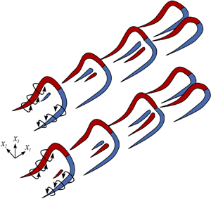
To visualize the three-dimensional vortical structures in the lobes and clefts of the gravity currents, figure 7 shows the swirling strength for the leading edge of the gravity current at  $Re=3450$ and the time instance is chosen at $t=3.14$ dimensionless units ( $\tilde {H} \tilde {u}^{-1}_b$). The swirling strength, $\lambda _{ci}$, is the absolute value of the imaginary part of the complex eigenvalue of the velocity gradient tensor and is suitable to pick out regions of intense vorticity. It corresponds to the part of vorticity associated with rotation and discriminates against the contribution made by shear (Chakraborty, Balachandar & Adrian Reference Chakraborty, Balachandar and Adrian2005; Adrian Reference Adrian2007). Our observations on the vortical structures in other cases in this study are qualitatively similar and only the vortical structures of the gravity current at $Re=3450$ are shown here. It is clear from figure 7 that an elongated tooth-like vortex forms the basis of a lobe and a pair of counter-rotating streamwise vortices are positioned on both the left- and right-hand sides of each cleft. As shown by the experiments of Simpson (Reference Simpson1972), McElwaine & Patterson (Reference McElwaine and Patterson2004), once the lobes and clefts form at the leading edge of the gravity currents, a cleft may continually merge with another neighbouring cleft while a new cleft may appear as a large lobe splits into two smaller ones. In what follows, we will investigate the merging of two clefts and the splitting of a lobe into two smaller ones by examining the vortical structures in the lobes and clefts.

Figure 7. Volumetric rendering of  $\lambda _{ci}$ for the gravity current propagating on a no-slip boundary at $Re=3450$. The time instance is chosen at $t=5.66$ dimensionless units ( $\tilde {H} \tilde {u}^{-1}_b$). Spacing between consecutive grid lines in the streamwise and spanwise directions, i.e. $x_1$ and $x_2$, is chosen at one tenth of a dimensionless unit.
3.2.1. Merging process
For illustrative purposes, here, we show a typical merging process in the lobe-and-cleft structure at the leading edge of the gravity current at  $Re=3450$. The location of the merging process which we are examining is marked as the blue circle in figure 4. To visualize the merging process, figure 8 shows the isosurface of the swirling strength ( $\lambda _{ci}=1.4$) at the leading edge of the gravity current at $Re=3450$ and the time instances are chosen at $t=5.66$ (a), $6.79$ (b), $7.92$ (c) and $9.05$ (d) dimensionless units ( $\tilde {H} \tilde {u}^{-1}_b$) throughout the merging process. The red and blue colours of the isosurfaces of the swirling strength represent the orientation of the vortex in the positive and negative streamwise directions, respectively. Prior to the merging, as shown in figure 8, there are three tooth-like vortices in the spatial range $0.3 < x_2 < 0.8$ and it requires three lobes, namely two clefts, to accomplish the merging process. As the two clefts approach each other, the middle lobe bounded by the two clefts shrinks in size. The middle tooth-like vortex breaks up into two legs, of which one leg reconnects with the left tooth-like vortex and the other leg reconnects with the right tooth-like vortex. These two reconnected vortical structures recede as the gravity current propagates forward and the two unbroken tooth-like vortices remain in the same place after the merging process.

Figure 8. Visualization from the top view of the merging of two clefts using the isosurface of the swirling strength  $\lambda _{ci}=1.4$ in the region $0 \le x_3^+ \le 36$ at $t=5.66$ (a), $6.79$ (b), $7.92$ (c) and $9.05$ (d) dimensionless units ( $\tilde {H} \tilde {u}^{-1}_b$) for the gravity current propagating on a no-slip boundary at $Re=3450$. The location of the merging process is shown in figure 4 by a blue circle.
The merging process can also be visualized by the streamwise velocity contours close to the bottom in the viscous wall region. Figure 9 shows the streamwise velocity and wall-normal velocity contours taken at a horizontal slice at  $x^+_3=x_3/\delta _\nu =8.6$ at the leading edge of the gravity current at $Re=3450$. Here, the vertical distance from the bottom boundary $x^+_3$ is measured in viscous length scale or wall unit. The spatial domain in figure 9 follows figure 8 and the time instances are likewise chosen at $t=5.66$ (a), $6.79$ (b), $7.92$ (c) and $9.05$ (d) dimensionless units ( $\tilde {H} \tilde {u}^{-1}_b$). The streamwise velocity is higher in the lobes than in the clefts and the wall-normal velocity is towards the bottom boundary in the lobes while the wall-normal velocity is away from the bottom boundary in the clefts. The locations of the clefts correspond to the locations of the low-speed streaks in figure 9. During the merging process, it is observed that the two low-speed streaks approach each other, as shown in figure 9(a,b) and a new low-speed streak develops, as shown in figure 9(c,d). The original two low-speed streaks prior to merging are disconnected from the new low-speed streak in the new cleft, as shown in figure 9(c,d). This typical merging process requires the interaction of three lobes. Therefore, a cleft may continually merge with another neighbouring cleft but may never disappear. Our observation on the merging of two clefts is consistent with the experimental investigations of Simpson (Reference Simpson1972), McElwaine & Patterson (Reference McElwaine and Patterson2004) in that clefts can only merge but never disappear and with the numerical investigation of Espath et al. (Reference Espath, Pinto, Laizet and Silvestrini2015) in that the merging process requires the interaction of three tooth-like vortices.

Figure 9. Visualization from the top view of the merging of two clefts using the streamwise velocity colour contours taken at a horizontal slice at  $x_3^+=8.6$ at $t=5.66$ (a), $6.79$ (b), $7.92$ (c) and $9.05$ (d) dimensionless units ( $\tilde {H} \tilde {u}^{-1}_b$) for the gravity current propagating on a no-slip boundary at $Re=3450$. Thin line contours show the wall-normal velocity with solid line for positive wall-normal velocity and dashed line for negative wall-normal velocity.
Following Dagaut et al. (Reference Dagaut, Negretti, Balarac and Brun2021), it would be interesting and instructive to look at the bottom friction coefficient, namely the dimensionless bottom shear stress, within the lobes and clefts. Figure 10 shows the dimensionless bottom shear stress at the leading edge of the gravity current at  $Re=3450$. Here, the spatial domain and time instances are chosen the same as figure 9. It is worth noting that the distribution of the bottom shear stress is similar to the streamwise velocity contour in that the bottom shear stress is higher in the lobes than in the clefts and the bottom shear stress continuously adjusts itself with the merging process.

Figure 10. Visualization from the top view of the dimensionless bottom shear stress  $\tau _b$ using colour contours at $t=5.66$ (a), $6.79$ (b), $7.92$ (c) and $9.05$ (d) dimensionless units ( $\tilde {H} \tilde {u}^{-1}_b$) for the gravity current propagating on a no-slip boundary at $Re=3450$.
3.2.2. Splitting process
As a new cleft forms, there exist a pair of counter-rotating streamwise vortices positioned on both the left- and right-hand sides of the cleft. Prior to splitting, however, there are no pre-existing counter-rotating streamwise vortices inside the splitting lobe. As such, the pair of counter-rotating streamwise vortices positioned on the left- and right-hand sides of the new cleft must develop themselves as the splitting process evolves.
For illustrative purposes, we examine a typical splitting process in the lobe-and-cleft structure at the leading edge of the gravity current at  $Re=3450$. The splitting process which we are now examining is located at the red cross symbol in figure 4 and, strictly speaking, the new cleft cannot be seen from the three-dimensional isosurface of density until $t=14.43$ dimensionless units ( $\tilde {H} \tilde {u}^{-1}_b$). Figure 11 shows the swirling strength at the leading edge of the gravity current at $t=12.45$ prior to the time when the new cleft manifests itself on the isosurface of density. At $t=12.45$, as shown in figure 11, there exists a tooth-like vortex which represents the lobe structure spanning $0.7 < x_2 < 1.2$. Additionally, at $x_1 \approx 12.8$ and $x_2 \approx 0.83$ there is a streamwise vortex which is smaller in size compared with the existing tooth-like vortex in the lobe and is closer to the bottom boundary. We shall term this smaller streamwise vortex the new born vortex. As time proceeds, the new born streamwise vortex grows in size and induces the other streamwise vortex of opposite orientation. The pair of counter-rotating streamwise vortices develop themselves and a new cleft forms in the splitting lobe. Based on our simulation results, the new born streamwise vortex can be either in the positive or in the negative streamwise direction. No preference over new born streamwise vortex in the positive or negative streamwise direction can be detected.

Figure 11. Three-dimensional top view of the initiation of the splitting process using the isosurface of the swirling strength  $\lambda _{ci}=1.6$ at $t=12.45$ dimensionless units ( $\tilde {H} \tilde {u}^{-1}_b$) for the gravity current propagating on a no-slip boundary at $Re=3450$. The location of the splitting process is shown in figure 4 by a red cross.
In order to identify the mechanism responsible for the creation of the new born streamwise vortex, we study the vorticity equation at the location where a lobe splits into two and the new cleft forms. We take the curl of the momentum equation (2.2) and the streamwise component of the vorticity equation is
 \begin{equation} \frac{\textrm{D} \omega_1 }{\textrm{D} t} = \underbrace{\omega_1 \frac{\partial u_1}{\partial x_1}}_{S_1} \underbrace{-\frac{\partial u_3}{\partial x_1} \frac{\partial u_1}{\partial x_2}}_{S_2} + \underbrace{\frac{\partial u_2}{\partial x_1} \frac{\partial u_1}{\partial x_3}}_{S_3} \underbrace{-\frac{\partial \rho}{\partial x_2}}_{S_4} + \underbrace{\frac{1}{Re} \nabla^2 \omega_1}_{S_5},\end{equation}
where  $S_1, S_2, S_3, S_4$ and $S_5$ represent the stretching of $x_1$ vorticity, twisting of $x_2$ vorticity, tilting of $x_3$ vorticity, baroclinic production of vorticity and diffusion of $x_1$ vorticity, respectively. We remark that the component $(\partial u_1/\partial x_3)(\partial u_1/\partial x_2)$ in the twisting of $x_2$ vorticity and the component $-(\partial u_1/\partial x_3)(\partial u_1/\partial x_2)$ in the tilting of $x_3$ vorticity have no net effects because they cancel exactly.
Figure 12 shows the contribution of the tilting of  $x_3$ vorticity, i.e. the $S_3$ term, to $D \omega _1 /Dt$ and the contribution of the baroclinic production of vorticity, i.e. the $S_4$ term, to $D \omega _1 /Dt$ at $t=11.88$ (a), $12.45$ (b), $13.01$ (c) and $13.58$ (d) dimensionless units ( $\tilde {H} \tilde {u}^{-1}_b$). It is worth noting that, prior to the new cleft appearing on the density isosurface, the contribution from the $S_3$ term comes inside the splitting lobe, as shown in figure 12(a). When the splitting process is initiated, the contribution from the $S_4$ term reinforces the $S_3$ term, as shown in figure 12(b–d), as the new cleft develops. The contributions of the stretching of $x_1$ vorticity, twisting of $x_2$ vorticity and diffusion of $x_1$ vorticity, i.e. the $S_1, S_2$ and $S_5$ terms, are less or even of opposite sign to the time rate of change of streamwise vorticity and are not shown for brevity. The signature of the Brooke–Hanratty mechanism (Brooke & Hanratty Reference Brooke and Hanratty1993) is that, close to the no-slip boundary, the largest contribution to the time rate of change of the streamwise vorticity, $\textrm {D} \omega _1/\textrm {D} t$, in the new born streamwise vortex comes from the tilting of $x_3$ vorticity, i.e. the $S_3$ term in (3.3). The baroclinic production of vorticity, i.e. the $S_4$ term in (3.3), was not seen in Brooke & Hanratty (Reference Brooke and Hanratty1993) for flows of a homogeneous fluid and is unique in the generation of vorticity in the lobe-and-cleft structure in gravity currents where density variation is essential. The baroclinic production of vorticity tends to consistently enhance the vorticity generated by the tilting of $x_3$ vorticity. As the pair of counter-rotating streamwise vortices develop and an indentation begins to show on the lobe, the baroclinic production of vorticity term generates positive streamwise vorticity on the right of the new cleft and negative vorticity on the left of the new cleft when looking in the positive streamwise direction. Therefore, the initiation of the splitting process can be attributed to the Brooke–Hanratty mechanism reinforced by the baroclinic production of vorticity. When the splitting process is initiated, a new born vortex, which is of opposite orientation to the parent vortex, can be created close to the bottom boundary at a location where the parent vortex lifts. The tooth-like vortex existing inside a lobe plays the role of the parent vortex and the new born vortex can be created by either the left part or the right part of the tooth-like vortex.

Figure 12. Visualization from the top view of the splitting process using the tilting of  $x_3$ vorticity, i.e. the $S_3$ term in (3.3), and the baroclinic production of vorticity, i.e. the $S_4$ term in (3.3), taken at a horizontal slice at $x^+_3=8.6$ at $t=11.88$ (a), $12.45$ (b), $13.01$ (c) and $13.58$ (d) dimensionless units ( $\tilde {H} \tilde {u}^{-1}_b$) for the gravity current propagating on a no-slip boundary at $Re=3450$. The contribution of the $S_3$ term is visualized by the colour contours and the positive and negative contributions of the $S_4$ term are represented by the thin solid and dashed lines, respectively. The thick solid line represents $\rho =0.1$ at $x^+_3=8.6$. The location of the splitting process is shown in figure 4 by a red cross.
An important manifestation of the Brooke–Hanratty mechanism in the creation of a new born vortex is the shifting of lobes at the leading edge of the gravity currents. The creation of a new born vortex occurs at a location where the parent vortex causes high-momentum fluid to impinge on the bottom boundary. The impingement of fluid onto the bottom boundary creates a high-pressure region and the fluid close to the bottom boundary is redirected in the spanwise direction. The appearance of the high-pressure region is associated with the shifting of the parent vortex away from the high-pressure region. As shown in figure 13(b) at  $t=12.45$, the parent vortex causes the impingement of fluid onto the bottom boundary and the new born vortex is created close to $x_2 \approx 0.83$. The parent vortex moves away from the high-pressure region and shifts in the negative spanwise direction (to the right in figure 13). This observation on the shifting of the parent vortex explains that the cleft, commencing at the red cross ( $x_1 \approx 13.92, x_2 \approx 0.81$) in figure 4, migrates in the negative spanwise direction as shown by the continuity of the cleft (dashed line) in figure 4.

Figure 13. Visualization from the back of the splitting process using the streamwise vorticity and velocity ( $u_2,u_3$) taken at a vertical cross-section. The streamwise vorticity is visualized by the colour contours with the solid and dashed lines indicating the positive and negative vorticity contours. The velocity is represented by the vectors. The four panels are taken at the streamwise location $x_1=12.70$ and the time $t=11.88$ (a), $x_1=12.90$ and $t=12.45$ (b), $x_1=13.13$ and $t=13.01$ (c), $x_1=13.36$ and $t=13.58$ (d) for the gravity current propagating on a no-slip boundary at $Re=3450$. The location of the splitting is shown in figure 4 by a red cross.
Depending on whether the parent vortex is in the positive (left part of the tooth-like vortex) or negative (right part of the tooth-like vortex) streamwise direction, the new born vortex can equally likely be in the negative or positive streamwise direction. For a new born vortex in the positive streamwise direction, the parent vortex, which is of opposite orientation of the new born vortex, must shift to the right of the new born vortex when looking in the streamwise direction, as shown in figure 14(a). Likewise, for a new born vortex in the negative streamwise direction, the parent vortex must shift to the left of the new born vortex when looking in the streamwise direction, as shown in figure 14(b). In either case, the shifting of the parent vortex makes room for the new born vortex and explains the direction of migration of the new cleft. As we have observed, a new cleft can equally likely shift in the positive or negative spanwise direction as the leading edge of the gravity currents moves forward in the streamwise direction. In the presence of a no-slip boundary, the lobe-and-cleft structure at the leading edge of the gravity currents is self-sustaining in that, while a cleft may continually merge with a neighbouring cleft, new clefts may form due to the Brooke–Hanratty mechanism reinforced by the baroclinic production of vorticity as long as the gravity currents continue to propagate forward. Encouragingly, our observations on the splitting of lobes and the migration of the clefts are in accord with the experimental observations of Simpson (Reference Simpson1972) and McElwaine & Patterson (Reference McElwaine and Patterson2004) in that the lobe-and-cleft structure is self-sustaining and the new cleft can equally likely shift in the positive or negative spanwise direction.

Figure 14. Sketch of the splitting process inside a lobe. Blue and red colours represent the vorticity in the negative and positive streamwise directions, respectively. In (a), the parent vortex is the right part (blue) of the tooth-like vortex and the new born vortex is in the positive (red) streamwise direction. In (b), the parent vortex is the left part (red) of the tooth-like vortex and the new born vortex is in the negative (blue) streamwise direction.
4. Conclusions
Gravity currents in the slumping phase from a full-depth lock-exchange configuration with a no-slip boundary are investigated by means of three-dimensional high-resolution simulations of the incompressible Navier–Stokes equations with the Boussinesq approximation. Our attention is focused on the evolution of the vortical structure and the mechanism responsible for the merging of clefts and splitting of lobes for the gravity currents propagating on a no-slip boundary.
Based on previously reported two-dimensional high-resolution simulations, only the thin layer of ambient fluid underneath the stagnation streamline in a translating coordinate system moving at the front speed, in which the head is held stationary, was thought to flow into the clefts. The ratio of the amount of ambient fluid going into the clefts to the total ambient volume flux, estimated based on the height of the stagnation streamline, decreases as the front Reynolds number increases. Our three-dimensional high-resolution simulations show that the lobe-and-cleft structure is of a three-dimensional nature. When the merging and splitting processes are at work, lobes of different sizes coexist at the leading edge of the gravity currents. Not only the ambient fluid underneath the stagnation streamline can be diverted around the lobes and into the clefts but also the ambient fluid above the stagnation streamline, if not flowing into the clefts directly, can do likewise. Due to the action of buoyancy, the ambient fluid inside the cleft region tends to rise in the head from the bottom boundary in mushroom-like shapes in the spanwise cross-sectional density contours. Quantitatively the estimates for the ratio of the amount of ambient fluid into the clefts to the total ambient volume flux based on the three-dimensional high-resolution simulations are significantly greater than the estimates based on previously reported two-dimensional simulations.
When the merging and splitting processes are at work, based on the three-dimensional simulations the overall mean lobe width and the mean of the maximum lobe width both agree with the empirical relationships originally proposed by Simpson (Reference Simpson1972). Furthermore, when measured in terms of the viscous length scale,  $\tilde {\delta }_\nu =\tilde {\nu }/\tilde {u}^*$ where $\tilde {\nu }$ is the kinematic viscosity of fluid and $\tilde {u}^*$ is the shear velocity at the gravity current head, the mean of the lobe width and the mean of the maximum lobe width both increase with increasing front Reynolds number from $60 \tilde {\delta }_\nu$ and $120 \tilde {\delta }_\nu$ at $Re_f = 383$ to $126 \delta _\nu$ and $230 \delta _\nu$ at $Re_f=3267$. The influence of the front Reynolds number gradually diminishes and the mean lobe width and the mean of the maximum lobe width approach asymptotically $126 \delta _\nu$ and $230 \delta _\nu$ at $Re_f=3267$, respectively.
The vortical structure inside a lobe has an elongated tooth-like shape and a pair of counter-rotating streamwise vortices are positioned on the left- and right-hand sides of each cleft. For the merging process, it requires the interaction of three tooth-like vortices and the middle tooth-like vortex breaks up and reconnects with the two neighbouring tooth-like vortices. Since the merging process requires the interaction of three tooth-like vortices, a cleft may continually merge with another neighbouring cleft but may never disappear. For the splitting process, a new born streamwise vortex is created by the parent vortex of opposite orientation, which can be either the left part or the right part of the existing tooth-like vortex inside the splitting lobe. This new born streamwise vortex then induces the other streamwise vortex of opposite orientation and a pair of counter-rotating streamwise vortices are positioned on the left- and right-hand sides of the developing new cleft. Depending on the orientation of the parent vortex, the new cleft develops after the splitting process can shift laterally in the positive or negative spanwise direction along the leading edge of the gravity currents as the lobe-and-cleft structure moves forward. The initiation of the splitting process can be attributed to the Brooke–Hanratty mechanism reinforced by the baroclinic production of vorticity. To the best of our knowledge, even though the lobe width has been measured in the experiments (Simpson Reference Simpson1972) and in the numerical simulations (Cantero et al. Reference Cantero, Balachandar and Garcia2007a,Reference Cantero, Lee, Balachandar and Garciab), there is no existing report in the literature that documents the evolution of the vortical structure inside the splitting lobe and the mechanism responsible for the splitting process. With the merging and splitting processes, the lobe-and-cleft structure is self-sustaining for the gravity currents propagating on a no-slip boundary and the manifestations of the merging and splitting processes in the lobe-and-cleft structure are in accord with reported laboratory observations.
Acknowledgements
A.D. is grateful for encouragement from Professors P. Linden and S. Dalziel at the University of Cambridge, S. Balachandar at the University of Florida, M. Garcia and G. Parker at the University of Illinois at Urbana-Champaign. Computational resources are provided by the Computer and Information Networking Center at National Taiwan University. The authors thank Mr C.-C. Li and Mr C.-H. Liang for their assistance in the project.
Funding
The research was supported financially by Taiwan Ministry of Science and Technology through grants MOST-109-2628-E-002-006-MY2.
Declaration of interests
The authors report no conflict of interest.


 Open access