


1. Introduction
The study of gravitational liquid curtain (sheet) flows issuing into an initially quiescent gaseous environment is particularly relevant for both technological and scientific aspects. On the one hand, working with steady liquid sheets falling under the influence of gravity is fundamental in several industrial applications, such as coating (Weinstein & Ruschak Reference Weinstein and Ruschak2004) and paper making (Soderberg & Alfredsson Reference Soderberg and Alfredsson1998) processes. On the other hand, the unsteady dynamics of curtain flow configurations is a matter of both historical (Brown Reference Brown1961; Lin Reference Lin1981; Weinstein et al. Reference Weinstein, Clarke, Moon and Simister1997; de Luca Reference de Luca1999) and ongoing (Torsey et al. Reference Torsey, Weinstein, Ross and Barlow2021; Chiatto & Della Pia Reference Chiatto and Della Pia2022; Colanera, Della Pia & Chiatto Reference Colanera, Della Pia and Chiatto2022) scientific studies. Among the challenges that remain open nowadays, there is the lack of an assessed theory able to predict the critical flow rate, namely the minimum value of the flow rate at which breakup phenomena of the curtain start to occur. The key dimensionless parameter involved in the problem is the Weber number  $We$, representing the relative importance between inertia and capillary effects. The pioneering experimental investigation carried out by Brown (Reference Brown1961) revealed that a necessary condition for the stability of the curtain is $We > 1$. He found the minimum liquid flow rate to guarantee the sheet stability by noticing that equilibrium must be maintained at a free edge between the inertia and surface tension forces. In particular, when a free edge appears because of the formation of a hole, such a hole does not grow if the sheet is in supercritical conditions ( $We > 1$), while it may produce the curtain disintegration in the subcritical regime ( $We < 1$). In the latter case, the liquid curtain exhibits an extremely rich variety of unstable behaviours, with several qualitatively different flow regimes that can be observed experimentally (among others, see Pritchard Reference Pritchard1986; de Luca & Meola Reference de Luca and Meola1995; Marston et al. Reference Marston, Thoroddsen, Thompson, Blyth, Henry and Uddin2014).
Therefore, it is evident that a topic of great importance in the analysis of liquid sheets disintegration is the dynamics of free edge holes forming inside the curtain flow. Various two-dimensional models have been proposed to face this problem from theoretical and numerical points of view (Sunderhauf, Raszillier & Durst Reference Sunderhauf, Raszillier and Durst2002; Savva & Bush Reference Savva and Bush2009; Deka & Pierson Reference Deka and Pierson2020; Agbaglah Reference Agbaglah2021a; Sanjay et al. Reference Sanjay, Sen, Kant and Lohse2022). However, these investigations did not take into account the influence of gravity acceleration on the free-edge retraction process. On the same research line, the early paper by Roche et al. (Reference Roche, Le Grand, Brunet, Lebon and Limat2006) and the recent contributions by Karim, Suszynski & Pujari (Reference Karim, Suszynski and Pujari2021) and Kyotoh, Sekine & Roknujjaman (Reference Kyotoh, Sekine and Roknujjaman2022) have studied the problem experimentally. Roche et al. (Reference Roche, Le Grand, Brunet, Lebon and Limat2006) focused on the liquid curtain response to localized perturbations of two different kinds, namely surface waves or free edges behind a thin needle touching the curtain, with a special emphasis on what happens near the breakup limit. The authors extracted and compared the shapes of two kinds of wakes left behind the obstacle: the classic triangular wake of standing sinuous waves, and a stationary hole involving two free edges pinned on the needle. It was found that the two perturbations behave similarly for high enough  $We$ values, but very differently when the Weber number reached the critical value $We=1$ by decreasing the inlet flow rate. In particular, the sinuous wake disappeared, whilst the hole-induced wake became rounded, and below $We=1$, the hole could stay stable, oscillate or expand and break the curtain. The last scenario was retrieved experimentally by Kyotoh et al. (Reference Kyotoh, Sekine and Roknujjaman2022) for relatively low Weber number values ( $0.2< We<0.6$).
The present work draws its motivation from the discussions reported above, and it is aimed at studying the hole-driven unsteady dynamics of a gravitational liquid curtain flow, in both supercritical ( $We>1$) and subcritical ( $We < 1$) conditions. The key point of the investigation is the use of a three-dimensional model of the flow system, which is fundamental to account for the effect of gravity on the hole rim propagation mechanisms inside the curtain. By performing three-dimensional direct numerical simulations with the volume-of-fluid method, the flow field features are first identified in steady conditions, by looking at the curtain interface shapes and the spatial distributions of velocity components. Afterwards, the hole-driven dynamics of the flow is analysed as the curtain response to a hole perturbation introduced artificially in the steady flow configuration, focusing on the combined influence of capillary retraction and gravity acceleration on the hole temporal evolution. The differences in the flow unsteady behaviour between supercritical and subcritical regimes are finally outlined, shedding light on the physical mechanisms leading to the curtain breakup in subcritical conditions. The influence of the curtain aspect ratio ${{AR}}$, namely the ratio between the curtain initial width and thickness, is also investigated, including the case of infinite ${{AR}}$ (i.e. edge-free curtain).
The work is organized as follows. In § 2, the numerical simulation framework is presented. Section 3 discusses the flow topology obtained in steady conditions, while § 4 presents results of the hole-driven curtain flow unsteady dynamics. Conclusions are drawn in § 5, and further details of the numerical solutions are provided in Appendices A and B.
2. Methodology
2.1. Theoretical framework and numerical modelling
The one-fluid formulation of incompressible Navier–Stokes equations (Scardovelli & Zaleski Reference Scardovelli and Zaleski1999) is employed to model the two-phase flow represented by the liquid curtain interacting with the initially quiescent gaseous environment:
 $$\begin{gather} \dfrac{\partial u^\star_i}{\partial x^\star_i}=0, \end{gather}$$
 $$\begin{gather}\rho\left( \dfrac{\partial u^\star_i}{\partial t^\star} + u^\star_j\,\dfrac{\partial u^\star_i}{\partial x^\star_j}\right)=-\dfrac{\partial p^\star}{\partial x^\star_i} + \rho g_i + \dfrac{\partial}{\partial x^\star_j} \left[\mu\left(\dfrac{\partial u^\star_i}{\partial x^\star_j} +\dfrac{\partial u^\star_j}{\partial x^\star_i} \right)\right] + F_\sigma, \end{gather}$$
 $$\begin{gather}\dfrac{\partial C}{\partial t^\star} + \dfrac{\partial C u^\star_i}{\partial x^\star_i}=0. \end{gather}$$
The vectors  $\boldsymbol {u}^\star = (u^\star,v^\star,w^\star )$ and $\boldsymbol {g} = (g,0,0)$ represent the flow velocity and the gravity acceleration, respectively, while $p^\star$ is the pressure. The force per unit volume due to the surface tension is denoted as $F_\sigma = \sigma \kappa ^\star n_i \delta _S$, where $\sigma$ is the surface tension coefficient, $\kappa ^\star$ is the mean gas–liquid interface curvature, and $\boldsymbol {n} = (n_x,n_y,n_z)$ is the outward pointing normal vector to the interface. The Dirac distribution function $\delta _S$ is equal to 1 at the interface, and 0 elsewhere. Note that all the dimensional quantities, except the gravity acceleration $g$ and the fluid material properties ( $\rho _l$, $\rho _a$, $\mu _l$, $\mu _a$, $\sigma$), are denoted with the superscript $\star$. The density $\rho$ and viscosity $\mu$ fields are discontinuous across the interface separating the two fluids, namely
 $$\begin{gather} \rho=\rho_a + (\rho_l -\rho_a)C , \end{gather}$$
 $$\begin{gather}\mu=\mu_a + (\mu_l -\mu_a)C , \end{gather}$$
where subscripts  $l$ and $a$ refer to liquid and ambient phases, respectively, and the volume fraction field $C$ is equal to either $1$ or $0$ in the liquid and gaseous regions.
The system (2.1a)–(2.1c) is solved using the finite volume method in the open-source code BASILISK (http://basilisk.fr), an improved version of Gerris (Popinet Reference Popinet2003) that has been used extensively and validated for several liquid jet flow problems (among others, see Della Pia, Chiatto & de Luca Reference Della Pia, Chiatto and de Luca2020; Schmidt & Oberleithner Reference Schmidt and Oberleithner2020; Agbaglah Reference Agbaglah2021b; Schmidt et al. Reference Schmidt, Tammisola, Lesshafft and Oberleithner2021). The code employs the volume-of-fluid method by Hirt & Nichols (Reference Hirt and Nichols1981) to track the interface on an octree structured grid, allowing for adaptive mesh refinement based on a criterion of wavelet-estimated discretization error (van Hooft et al. Reference van Hooft, Popinet, van Heerwaarden, van der Linden, de Roode and van de Wiel2018), with no special treatment required in the presence of liquid phase breakup. The calculation of the surface tension term is based on the balanced continuum surface force technique (Francois et al. Reference Francois, Cummins, Dendy, Kothe, Sicilian and Williams2006), which is coupled with a height-function curvature estimation to avoid the generation of spurious currents. For exhaustive details about BASILISK, the reader is referred to Popinet (Reference Popinet2003, Reference Popinet2009).
2.2. Geometrical layout and problem formulation
A schematic description of the computational domain is reported in figure 1(a), where the gravity direction is denoted by  $x$. The domain is a cubic region extending along the $x$ (streamwise), $y$ (transverse) and $z$ (spanwise) directions, where $L^\star = 50 H^\star _i$ is the domain side length. The spatial coordinates $x$,
$x$,  $y$ and $z$ have been scaled with respect to the inlet (i.e. at the streamwise station $x=0$) sheet thickness $H^\star _i$ (namely $x=x^\star /H^\star _i$), while the corresponding streamwise $u$, transverse $v$ and spanwise $w$ velocity components have been made dimensionless with respect to the inlet mean liquid velocity $U^\star _i$ ( $u = u^\star /U^\star _i$).

Figure 1. (a) Schematic representation of the computational domain, and (b) inflow velocity profile (2.3a). The gravity  $g$ is directed along the streamwise direction $x$;
$x$;  $y$ is the lateral coordinate, and $z$ is the spanwise one.
The curtain issues into an initially quiescent gaseous environment (blue region in figure 1) from a rectangular slot of dimensions  $H^\star _i \times W^\star _i$, representing the initial thickness (along the transverse $y$ coordinate) and width (along the spanwise $z$ direction) of the sheet, respectively. The origin of the reference frame coincides with the centre of the slot, and the curtain shape is initialized as a parallelepiped with volume $L^\star \times H^\star _i \times W^\star _i$ (red region in figure 1a), which is employed to start the computation. Dirichlet boundary conditions are enforced at the inlet: following Kacem (Reference Kacem2017), in the liquid region ( $-1/2< y<1/2$, $-{{AR}}/2< z<{{AR}}/2$, where ${{AR}} = W^\star _i/H_i^\star$ is the sheet aspect ratio), a fully developed parabolic velocity profile with a proper error function modification is imposed to account for viscous effects at the slot boundaries ( $y = \pm 1/2$, $z = \pm {{AR}}/2$), and the conditions read
 $$\begin{gather} u=\dfrac{3}{2}\left(1 - 4y^2 \right) \text{erf} \left(\dfrac{{{AR}}}{2} - z\right) \text{erf} \left(\dfrac{{{AR}}}{2} + z\right), \end{gather}$$
 $$\begin{gather}v = w=0, \end{gather}$$
 $$\begin{gather}C=1 . \end{gather}$$
On the remaining part of the inlet plane, namely within the gaseous phase, a no-slip condition is imposed; the inflow velocity profile  $u(x=0,y,z)$ is represented in figure 1(b). The four lateral boundary planes ( $y= \pm 25$, $z= \pm 25$) are equipped with homogeneous Neumann boundary conditions for all variables, and on the outlet plane ( $x=50$) a standard outflow condition
 $$\begin{gather} \dfrac{\partial u}{\partial x} = \dfrac{\partial v}{\partial x}=\dfrac{\partial w}{\partial x} = \dfrac{\partial C}{\partial x}=0, \end{gather}$$
 $$\begin{gather}p=0, \end{gather}$$
is considered. The same  $u(y,z)$ profile enforced as inlet boundary condition (2.3a) is also employed as the initial velocity distribution throughout the entire sheet length. We note here explicitly that a slight modification of the initial and boundary conditions presented above is required to obtain the last results reported in § 4.3. In particular, to simulate an edge-free curtain flow, homogeneous Neumann boundary conditions are replaced by periodic conditions on the lateral walls of the domain. Moreover, the parallelepiped curtain shape employed as initial condition is extended all along the spanwise direction, thus matching the whole domain side length.
The computational domain is discretized with an adaptive mesh up to a maximum number of  $2^9$ grid points along each spatial dimension, corresponding to a minimum mesh size $\varDelta ^\star \approx H^\star _i/11$, and approximately $134$ million cells if a uniform grid was used; the mesh resolution effect on the results hereafter presented is reported in Appendix A. Note that recently, a resolution $\varDelta ^\star / H^\star _i \approx 6$ has been shown by Agbaglah (Reference Agbaglah2021a) to be valuable in capturing holes expansion and collision in a thin liquid sheet.
The  $n=10$ physical quantities involved in the problem ( $\rho _l$, $\rho _a$, $\mu _l$, $\mu _a$, $g$,
$g$,  $U^\star _i$, $W^\star _i$, $H^\star_i$, $L^\star$, $\sigma$) can be rearranged in $m=n-3$ independent dimensionless numbers: a possible choice is reported in table 1 ( $r_\rho$, $r_\mu$, $\varepsilon$, ${{AR}}$, $Re$,
$Re$,  $Fr$,
$Fr$,  $We$), which also specifies a set of numerical values corresponding to the reference configuration analysed in § 3. Following Chubb et al. (Reference Chubb, Calfo, McConley, McMaster and Afjeh1994), the Froude number is based on the curtain width $W_i^\star$. Note that a different arrangement of the dimensional parameters leads to the definition of the Ohnesorge number $Oh = \mu /\sqrt {2 H^\star _i \rho _l \sigma }$, whose value is also reported in table 1.
Table 1. Dimensionless governing parameters and their values for the reference case.

3. Steady flow configuration
The curtain flow steady solution for the supercritical ( $We=2.5$) reference case specified in table 1 is shown in figure 2 in terms of three-dimensional interface shape (figure 2a), contour representation of the spanwise velocity component $w$ within the $xz$ plane ( $y=0$, figure 2b), and velocity profiles at different streamwise $x$ stations in the same plane (figure 2c).

Figure 2. (a) Three-dimensional view of the liquid sheet interface. (b) Map of spanwise velocity field  $w$ in the $xz$ plane. (c) Profiles of $w(z)$ at different streamwise $x$ stations for $y=0$. Steady flow, $We=2.5$, ${{AR}}=40$.
Starting from the parallelepiped shape initialization described previously in § 2.2, steady flow conditions are achieved after a computational time approximately  $t^\star = 1.0\,L^\star /U^\star _i$. In the steady flow configuration, the curtain exhibits the characteristic triangular shape (figure 2a) outlined by previous theoretical analyses and experimental investigations (among others, Chubb et al. Reference Chubb, Calfo, McConley, McMaster and Afjeh1994; de Luca & Meola Reference de Luca and Meola1995; Kacem et al. Reference Kacem, Le Guer, El Omari and Bruel2017; Jaberi & Tadjfar Reference Jaberi and Tadjfar2017). The triangular shape is determined by the edges retraction and convergence towards the central axis ( $z=0$), which is an effect of the surface tension force acting on the curtain lateral edges. By inspection of the three-dimensional interface, it is possible to observe striped patterns indicating the presence of surface capillary waves, which manifest as stationary ripples in the transition area between the lateral edges and the planar part of the sheet, resulting from the competition between viscous and capillary forces. The dimensionless parameter representing the relative importance between viscous and surface tension effects is the Ohnesorge number, which in the present case is $Oh= 0.002 \ll 1$. This leads to the formation of capillary waves near the edges, as predicted theoretically and numerically by Sunderhauf et al. (Reference Sunderhauf, Raszillier and Durst2002), Savva & Bush (Reference Savva and Bush2009), Pierson et al. (Reference Pierson, Magnaudet, Soares and Popinet2020), Deka & Pierson (Reference Deka and Pierson2020) and Karim et al. (Reference Karim, Suszynski and Pujari2021), and observed experimentally by Kacem et al. (Reference Kacem, Le Guer, El Omari and Bruel2017).
The spatial evolution of ripples is quantified by showing the spanwise velocity component  $w(x,z)$ contour (figure 2b) and the profiles $w(z)$ at different $x$ stations (figure 2c) in the $xz$ plane ( $y=0$). At $x=5$ (black curve in figure 2c), the velocity oscillates between negative and positive values near the lateral rims, and it drops down steeply in the region between the edge and the inner part of the curtain; the same behaviour was highlighted by Sunderhauf et al. (Reference Sunderhauf, Raszillier and Durst2002) in the study of the edge retraction of a planar liquid sheet for low $Oh$ values (see in particular figure 8 in Sunderhauf et al. Reference Sunderhauf, Raszillier and Durst2002). Moving along the streamwise $x$ direction, further crests appear, starting from the curtain edges, which are displaced towards the central part of the sheet due to the rim retraction (as depicted by the black, red and blue curves in figure 2c). As a combined effect of gravity acceleration and rims retraction, the waves coming from the edges interfere with each other for $x > 20$, producing a criss-cross pattern, as also found experimentally by Kacem et al. (Reference Kacem, Le Guer, El Omari and Bruel2017).
The competition between gravity and surface tension determines a streamwise variation of the spanwise velocity  $w$ at the edges, with values ranging from 0.5 to 0.9 for $x \in [5,25]$. The order of magnitude of $w$ agrees with the theoretical prediction of the rim retraction velocity given by the Taylor–Culick model (Taylor Reference Taylor1959; Culick Reference Culick1960), hereafter made dimensionless by means of $U^\star _i$:
 \begin{equation} u_c = \dfrac{1}{U^\star_i}\sqrt{\dfrac{2 \sigma}{\rho_l H^\star_i}} = 0.63, \end{equation}
a reference value that accounts for neither the vertical gravity acceleration nor viscous effects. Of course,  $We=1/u_c^2=2.5$. From figures 2(b,c), we also note that the ripples wavelength (made dimensionless with respect to $H^\star _i$), estimated as the distance between two successive peak values of $w$ in the central part of the sheet (blue curve in figure 2(c) for $-5< z<5$) is approximately $\lambda _c= 1.85$, in good agreement with the capillary length $l_c = ({1}/{H^\star _i})\sqrt {{\sigma }/{\rho _l g}} = 1.81$, representing a typical length scale in flows driven by capillary effects. A similar value $\lambda _c=1.63$ has been found recently in the study of an axisymmetric filament retraction at low $Oh$ and high aspect ratio values by Pierson et al. (Reference Pierson, Magnaudet, Soares and Popinet2020) (see the discussion on page 11 of Pierson et al. Reference Pierson, Magnaudet, Soares and Popinet2020), who scaled the wavelength with respect to the filament diameter. Furthermore, it can be appreciated from figure 2(b) that the sheet evolution perturbs the initially quiescent ambient phase, which manifests the phenomenon of gas entrainment, that is, $w < 0$ ( $> 0$) for $z > 0$ ( $<0$) outside the curtain.
The overall flow topology is elucidated further by observing the curtain interface shapes in three cross-sections taken with planes parallel to the  $x=0$ plane, namely $x=5$, $15$ and $25$ (figure 3a), together with the colour maps of spanwise $w$ and transverse $v$ velocity components within the liquid phase at $x=15$ (figures 3(b) and 3(c), respectively). As the curtain width reduces along the streamwise direction, the rim thickness increases (figure 3a) and the capillary ripples are displaced towards the curtain centre, thus producing varicose patterns (i.e. symmetric with respect to the $y=0$ axis) and associated transverse $v$ velocity distributions in $yz$ planes.

Figure 3. (a) Interface shape in  $yz$ planes located at different $x$ stations. Maps of (b) spanwise $w$ and (c) transverse $v$ liquid velocity components at $x=15$. Steady flow, $We=2.5$, ${{AR}}=40$.
The variation of the streamwise velocity component  $u(x,y)$ in the $z=0$ plane within the liquid phase is reported in figure 4(a), while the comparison between various estimates of the centreline streamwise velocity is illustrated in figure 4(b). In particular, the latter figure compares the $u$ streamwise trend for $y=0$ (red line) with the $y$-averaged velocity in the $xy$ plane (black continuous line), defined as
 \begin{equation} \langle u \rangle(x) = \dfrac{1}{{\int_{-H/2}^{H/2} C(x,y)\, {{\rm d} y}}}\boldsymbol{\cdot} \int_{-H/2}^{H/2} C(x,y)\,u(x,y) \,{{\rm d} y}, \end{equation}
where  $H=H^\star /H^\star _i$. The free-fall Torricelli's theoretical solution (black dashed line)
 \begin{equation} u_{Torr}=\sqrt{1+\dfrac{2}{{{AR}}}\,\dfrac{x} {Fr}} \end{equation}
is also reported for comparison, with  $Fr$ being the Froude number defined in table 1.

Figure 4. (a) Map in the  $xy$ plane of the streamwise liquid velocity $u$. (b) The $x$-variation of the axial velocity $u(x,y=0)$ and $y$-averaged trend $\langle u \rangle (x)$. The reference Torricelli's velocity $u_{Torr}$ and the calculated convergence length $L_c$ are also reported in (b). Steady flow, $We=2.5$, ${{AR}}=40$.
The analysis of figure 4 allows one to distinguish three different regions of the steady flow field. In the first region, extending from  $x=0$ to approximately $x=20$, the curtain develops nearly two-dimensionally in the $xy$ plane, namely the velocity field agrees with that predicted by strictly two-dimensional simulations of the flow (see, for example, figure 5 of Della Pia et al. Reference Della Pia, Chiatto and de Luca2020). In particular, due to the gravity action, the sheet thickness reduces and the streamwise velocity increases. Moreover, the initial parabolic velocity profile (2.3a) relaxes towards a quite plug distribution, as shown by the convergence between the axial value of the velocity $u(x,y=0)$ and the one-dimensional reduction $\langle u \rangle (x)$, which agrees well with the theoretical value $u_{Torr}$ as $x$ increases. The second region is located in the range $20< x< L_c$, being in the present case $L_c = 32.19$, the rims convergence length, where the streamwise velocity displays an oscillating trend (see the superposition of red and black continuous curves) as a result of the interference between surface capillary waves coming from the right and left edges outlined previously in figure 2(b). Finally, in the third region ( $x > L_c$), the sheet is characterized by a tail with increasing thickness in the $xy$ plane, denoting an incipient axis switching effect (among others, see the recent experimental investigation by Jordan et al. Reference Jordan, Ribe, Deblais and Bonn2022). Note that the convergence length $L_c$ has been calculated as the $x$ value corresponding to the maximum of $u(x,y=0)$, i.e. minimum of the curtain thickness within the $xy$ plane.
The present numerical estimate of  $L_c$ agrees with the simplified theoretical prediction by Chubb et al. (Reference Chubb, Calfo, McConley, McMaster and Afjeh1994),
 \begin{equation} L^{th}_c =\dfrac{Fr\,{{AR}}}{2}\left[\left(1+\dfrac{3}{2\,Fr}\,\sqrt{\dfrac{We}{8}} \right)^{{4}/{3}} -1\right], \end{equation}
as shown in table 2. As a matter of fact, for  ${{AR}}=40$ and the range $We \in [1.5,2.5]$, the relative percentage spread $\epsilon _c = 100 (L_c - L^{th}_c)/L_c$ is less than $15\,\%$. It is worth noticing that numerical simulations at the different Weber number values have been performed by decreasing the inlet velocity $U^\star _i$, thus determining a corresponding reduction of the Froude number $Fr$, as highlighted in table 2. The variation of the convergence length $L_c$ with the Weber number is also shown in figure 5, together with the theoretical prediction $L^{th}_c$.
Table 2. Comparison between theoretical ( $L^{th}_c$, (3.4)) and numerical ( $L_c$) values of the convergence length by varying Weber and Froude numbers. The relative percentage spread is defined as $\epsilon _c = 100\ (L_c - L^{th}_c)/L_c$. Here, ${{AR}}=40$.


Figure 5. Convergence length  $L_c$ variation with the Weber number $We$. The theoretical prediction $L^{th}_c$ (3.4) is also reported. Here, ${{AR}}=40$.
4. Hole-driven unsteady dynamics
Since the experimental evidence of the curtain breakup can be linked to the formation and amplification of a hole in its frontal plane (among others, see Roche et al. Reference Roche, Le Grand, Brunet, Lebon and Limat2006; Kyotoh et al. Reference Kyotoh, Sekine and Roknujjaman2022), its unsteady dynamics is analysed in this section as the response to the presence of a hole introduced artificially in the steady flow. In particular, a cylindrical hole of diameter equal to  $H^\star _i$, centred at a certain streamwise station $x_h$ and $z_h=0$, is superimposed on the steady solution along the entire curtain thickness. The equation describing the (dimensionless) initial hole region in the $xz$ plane is
 \begin{equation} (x-x_h)^2 + z^2 \leq \tfrac{1}{4}, \end{equation}
which gives rise to a toroidal rim at the free end of the hole after few time steps (see also Agbaglah Reference Agbaglah2021a). The streamwise location of the hole centre is first chosen equal to  $x_h=10$, to perform the analysis in both supercritical ( $We > 1$) and supercritical-to-subcritical ( $We < 1$) transition conditions, respectively in §§ 4.1 and 4.2. The hole is then moved upstream at $x_h=2$ to investigate the subcritical regime, where an edge-free curtain flow is considered, as will be motivated and discussed in § 4.3.
4.1. Supercritical regime
The unsteady behaviour of the curtain shape in the  $xz$ plane influenced by the time evolution of the hole is shown qualitatively in figure 6 and quantified in figure 7. The temporal evolution of the curtain shape is depicted in figure 6 in terms of volume fraction $C$ contour maps. Following the approach by Karim et al. (Reference Karim, Suszynski and Pujari2021), the trajectories of three representative points of the hole are monitored in figure 7, namely the northernmost $x_N(t)$ (red), southernmost $x_S(t)$ (blue) and centre $x_{C}(t)$ (green) points of the hole. The analysis is performed for a relatively low supercritical Weber number value $We=1.1$, for which surface tension is expected to have a relatively strong influence on the hole-driven curtain dynamics. The aspect ratio is ${{AR}}=40$. Note that the temporal variable $t$ in figures 6 and 7 is scaled with respect to the reference time $t^\star _{ref} = H^\star _i/u^\star _c$, the hole being introduced at $t=0$ in the steady curtain configuration.

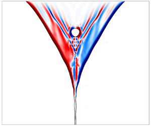
Figure 6. Maps of volume fraction  $C$ in the $xz$ plane at different time instants. The liquid phase is represented in red, the gaseous phase in blue. Here, $We = 1.1$, ${{AR}}=40$, with (a) $t = 0$, (b) $t = 1$, (c) $t = 2.2$, (d) $t = 3.3$, (e) $t = 4.9$, (f) $t = 6.7$, (g) $t = 7.4$, (h) $t = 8.6$, (i) $t = 10.2$.

Figure 7. (a) Hole initial shape in the  $xz$ plane. (b) Curtain shape around the hole region in the $xy$ plane. (c) Hole northernmost $x_N(t)$ (red curve), southernmost $x_S(t)$ (blue curve) and centre $x_{C}(t)$ (green curve) points trajectories in the $xz$ plane. In (a,b), the liquid phase is shaded in red, with the gaseous phase in blue. Here, $We = 1.1$, ${{AR}} = 40$.
Following the sequence in figure 6, it can be noted that the initially circular hole is advected downstream progressively while undergoing a continuous shape deformation, until it closes and leaves the sheet intact. In the early stages of the evolution ( $t < 3.3$), the temporal variation of the curtain shape is influenced only by the competition between the hole rim retraction, due to the surface tension acting on the hole perimeter, and the hole fall motion, determined mainly by the streamwise-oriented gravity force. As for the $x_N(t)$ motion, the surface tension counteracts gravity, the two forces having opposite directions in the northernmost point of the hole, while they are both directed downstream in the southernmost one (see figures 7a,b). This determines a progressive stretching of the hole along the streamwise direction (figures 6a–c), with a falling velocity $\dot{x}_N = 1.0$ smaller than $\dot{x}_S = 3.6$, as can be appreciated by the different initial slopes of the red and blue curves in figure 7(c); the streamwise velocity of the hole centre assumes a value $\dot{x}_{C} = 2.2$ (slope of the green curve in figure 7c). It is straightforward to verify that the orders of magnitude of these velocities are consistent with each other. As a matter of fact, if one assumes that the velocity of the hole centre point is essentially the falling velocity of the main liquid stream, then the velocities of the northernmost and southernmost points of the hole can be estimated by subtracting and adding, respectively, to the centre point velocity the ‘net’ rim retraction velocity, whose order of magnitude is given by the Taylor–Culick model (which is of unit order in dimensionless scale).
At intermediate stages ( $3.3< t<8.6$), the hole dynamics starts to be influenced by the lateral edges of the curtain, namely the hole no longer expands freely. The curtain edges slow down the overall expansion (figures 6d–g), determining a reduction of the velocity $\dot{x}_S$ from 3.6 to 0.9 (figure 7(c) at $t=3.3$). The hole thus assumes a triangular shape, analogously to the underlying liquid sheet. Finally, during the last stages of the evolution ( $t > 8.6$), the hole expansion is counteracted not only by the curtain edges, but also by the approaching vertical tail (figures 6h,i). Therefore, the streamwise stretching and the overall expansion of the hole stop: the southernmost point velocity becomes negative ( $\dot{x}_S = -2.3$; see figure 7(c) at $t=9.0$), thus leading to the closure of the hole before it reaches the outlet section of the physical domain, i.e. the curtain length.
The hole dynamics in  $yz$ planes is shown qualitatively in figure 8 and quantified in figure 9. Figures 8(a,b) depict the temporal evolution of the hole rim shape of the right hemi-curtain (i.e. for $z>0$) in two $yz$ planes located at the streamwise stations $x=13$ and $x=19$, respectively. Note that the geometrical features of the shapes significantly recall the elliptic, cigar-like and peanut-like shapes found in the pioneering combined theoretical–experimental investigation by Chubb et al. (Reference Chubb, McConley, McMaster and Afjen1993). The spanwise positions of the hole rim tip $z_T$ (leftmost point of the hole, denoted by the arrows in figure 8) and the retraction velocity $w_T= \dot{z}_T$ at the same streamwise stations are shown in figures 9(a,b) and 9(c,d), respectively, for $x=13$ and $x=19$, where the retraction velocity is scaled with respect to the Taylor–Culick reference value, i.e. $w_T = w^\star _T/u^\star _c$. Note that the time interval considered in each panel is computed as $\Delta t = t-t^0_h(x)$, where $t^0_h(x)$ is the time instant when the hole reaches the streamwise $x$ location. Since the hole grows progressively, moving along the streamwise direction for $x \in [0,20]$, as shown in figures 6 and 7 discussed previously, the time interval $\Delta t$ at $x=19$ (figures 8b and 9c,d) is greater than the corresponding interval at $x=13$ (figures 8a and 9a,b).

Figure 8. Temporal evolution of the hole rim shape in the  $yz$ planes for the right hemi-curtain (i.e. $z>0$) for (a) $x=13$, and (b) $x=19$. The liquid phase is shaded in red, the gaseous phase in blue. The arrows denote the hole tip. Here, $We=1.1$, ${{AR}} = 40$.

Figure 9. Spanwise position  $z_T$ and velocity $w_T$ of the hole rim tip in $yz$ planes (right hemi-curtain for $z>0$) as a function of time, for (a,b) $x=13$, and (c,d) $x=19$. The dashed lines in (b,d) denote the values $w^\star _T/u^\star _c= \pm 1$. Here, $We=1.1, {{AR}} = 40$.
The time evolution of the sheet shape reported in figures 8(a,b) exhibits a fast retraction of the rim at the early instants, at both  $x=13$ and $x=19$, after its abrupt formation when the hole reaches the two streamwise stations. This can be appreciated qualitatively by looking at the large distance between the green and red curves at $y=0$, and it is quantified by the relatively higher slope of curves $z_T$ and $w_T$ at small $\Delta t$ values in figure 9. At later stages, the rim motion slows down, and the tip position $z_T$ reaches a maximum (for $\Delta t = 1.2$ and $2.1$, at $x=13$ and $19$, respectively) and then decreases. This corresponds to an inversion of the retraction process, due to the advection of the hole along the streamwise direction (blue and black curves in figure 8), which finally leaves both the $yz$ planes at relatively large time instants ( $z_T = 0$ for $\Delta t = 2.5$ and $5.5$, at $x=13$ and $19$, respectively).
The main difference between the hole curtain dynamics at the two streamwise stations considered here is due to the increasing effect of the curtain edges as  $x$ increases. At the upstream station, $x=13$, the edges are relatively far from the hole, which expands freely under the effect of surface tension. The hole-driven rim dynamics is thus characterized by a monotonic decreasing trend of the retraction velocity $w_T$, which eventually assumes negative values when the hole progressively leaves the station. On the contrary, the hole-induced rims are relatively close to the curtain edges at the downstream station, $x=19$, causing a mutual interaction that produces an oscillatory behaviour of the velocity $w_T$ in the range $w_T \in [-1,1]$, before the hole finally approaches the curtain tail.
To justify the relatively high values of the retraction velocity  $w_T$ of the tip point, one should consider that the hole is immersed in a flow field subjected to the gravity acceleration. As a consequence, the ‘total’ retraction velocity of the left tip of the hole is given by the substantial derivative
 \begin{equation} w_T = \dfrac{\partial z_T}{\partial t} + u\,\dfrac{\partial z_T}{\partial x}, \end{equation}
where the unsteady term  ${\partial z_T}/{\partial t}$ represents the pure retraction contribution usually modelled by the Taylor–Culick velocity, and the convective term $u ({\partial z_T}/{\partial x})$ is the tip displacement rate due to the local slope of the hole (in the $xz$ plane) advected downstream with velocity $u$. The convective term is indeed significant only when the hole tip at the given station $x$ corresponds to the maximum of the absolute value $|\partial z_T /\partial x|$ (i.e. the hole tip in the $yz$ plane coincides with the northernmost hole point in the $xz$ plane). On the contrary, the convective derivative is negligible when the hole tip coincides with the hole leftmost point in the $xz$ plane, so that the order of magnitude of $w_T$ coincides with the Taylor–Culick velocity, namely $w_T = \partial z_T/\partial t = {O}(1)$.
To sum up, the main result arising from the analysis performed in this section is that in supercritical conditions, the hole perturbation introduced in the curtain does not influence the dynamics of the flow at large times. Indeed, whilst the hole undergoes an initial transient expansion, its interaction with the curtain borders determines first a slowdown and then a reversal of the expansion process, thereby producing the hole closure upstream of the sheet exit section (see also supplementary movie 1 available at https://doi.org/10.1017/jfm.2023.543).
4.2. Transcritical regime
The unsteady dynamics of the curtain in transcritical conditions is studied by considering two values of the Weber number close to the critical unit threshold, namely  $We=1.1$ (as in § 4.1) and $We=0.95$.
The time evolution of the hole area  $A^\star$ with respect to its initial value $A^\star _i$ is reported in figure 10, respectively for $We=1.1$ (black curves) and $We=0.95$ (red curves). The trend of both curves reported in figure 10(a) is the same: the hole area first increases due to the hole expansion at the early stages of its evolution, reaches a maximum at the peak time $t=t_{p}$, and then decreases to zero due to the hole closure process. Although the supercritical and subcritical behaviours are qualitatively analogous, two main differences can be detected. First, both the peak time $t_{p}$ and the corresponding area amplification $A^\star _p/A^\star _i$ are greater for $We=1.1$ ( $t_{p} = 3.3$, $A^\star _p/A^\star _i = 58$) than for $We=0.95$ ( $t_{p} = 2.7$, $A^\star _p/A^\star _i = 44$). Moreover, the initial amplification rate is higher for $We=0.95$ rather than $We=1.1$, as can be appreciated more clearly by looking at figure 10(b). The two curves are characterized by an exponential growth at the early time instants, $A^\star /A^\star _i = {\rm e}^{\alpha t}$, with the hole expansion rate $\alpha$ increasing from $\alpha =5/2$ to $\alpha =4$ by reducing the Weber number from supercritical to subcritical conditions. It is interesting to note that an exponential growth of hole amplifications inside two-dimensional liquid sheets was also found in the combined theoretical–numerical investigation by Savva & Bush (Reference Savva and Bush2009), who performed simulations in the high viscous limit ( $Oh \gg 1$) and did not consider the effect of gravity on the hole dynamics. On the other hand, here $Oh \ll 1$ (see table 1 in § 2.2) and gravitational effects are fully taken into account.

Figure 10. (a) Time evolution of the hole area  $A^\star$ with respect to its initial value $A^\star _i$ at the supercritical-to-subcritical flow transition; (b) zoom around the first time instants. Black curves denote $We=1.1$, and red curves denote $We=0.95$. The peak time $t_p$ and the corresponding area amplification are also highlighted in (a) for the case $We=1.1$. Here, ${{AR}}=40$.
Analogies and differences between the  $We > 1$ and $We < 1$ cases can be explained easily by recalling the discussion in § 4.1 about the physical mechanisms involved in the hole dynamics. At the early stages of the evolution, the hole expands freely under the effect of the surface tension acting on its rims, which is clearly stronger in the subcritical rather than supercritical regime, thus determining a faster expansion of the area in the former case. On the other hand, as soon as the hole approaches the central vertical region of the curtain, the surface tension acting on the curtain edges counteracts the hole expansion, the effect being again stronger for $We < 1$ than for $We > 1$, thus determining an earlier decay (and consequently a lower maximum of the hole area) of the subcritical curve. The same considerations can be retrieved by looking at figure 11, which reports the hole northernmost ( $x_N(t)$) and southernmost ( $x_S(t)$) points trajectories for $We=1.1$ and $We=0.95$ (black and red curves, respectively). Moreover, the analysis of figure 11 reveals that in the transition from supercritical to subcritical flow regimes, the hole northernmost point velocity (slope of $x_N(t)$ curves) decreases slightly. Scaled with respect to the Taylor–Culick reference value $u^\star _c$, the velocity reads as $\dot{x}^\star _N/u^\star _c = 1.0$ for $We=1.1$, and $\dot{x}^\star _N/u^\star _c =0.8$ for $We=0.95$, respectively.

Figure 11. Hole northernmost  $x_N(t)$ and southernmost $x_S(t)$ points trajectories in supercritical-to-subcritical flow transition conditions. Here, ${{AR}}=40$.
4.3. Edge-free subcritical regime
In the previous sections we observed that the dynamics of a hole introduced in the falling liquid sheet is influenced crucially by the presence of the lateral free edges of the curtain itself, determining a slowdown of the hole advected by the main stream, in both supercritical and weakly subcritical regimes. In this respect, there is no discontinuity in the sheet behaviour when traversing the critical Weber threshold. On the other hand, it has also been found that for finite values of the aspect ratio  ${{AR}}$, the steady curtain flow configuration can no longer be achieved for lower $We$ numbers (e.g. for $We<0.8$), due to the spontaneous appearance of various irregular holes interacting with each other inside the sheet. This occurrence will be illustrated in Appendix B.
To address the analysis of the free dynamics of the hole, namely not influenced by the lateral edges of the sheet, the configuration of infinite  ${{AR}}$ is investigated in the present section, for various subcritical $We$ numbers. This study has been performed by locating the hole perturbation (4.1) at a station further upstream, namely $x_h=2$. Moreover, by employing periodic boundary conditions on the lateral walls of the domain (see the discussion reported in § 2.2), the edge-free curtain flow has been simulated.
The time evolution of the curtain shape in the  $xz$ plane is reported in figure 12 for the slightly subcritical Weber number value equal to $We=0.9$. It can be seen that in the absence of the curtain borders, the hole expands in a wide region (figures 12a–c) while it is convected downstream by the gravitational acceleration (figures 12d–f). As time increases further, the hole is expelled progressively at the outlet section (figures 12g,h), leaving the liquid curtain in its original unperturbed configuration (figure 12i). It is also worth noticing that by simulating the edge-free curtain flow in supercritical conditions ( $We=1.1$), we retrieved the same overall behaviour outlined in figure 12. For the sake of brevity, edge-free supercritical curtain flow simulations have not been reported herein.

Figure 12. Time evolution of the volume fraction  $C$ in the $xz$ plane of an edge-free curtain in slightly subcritical conditions ( $We=0.9$). Time $t$ increases from (a) to (i), as (a) $t = 0$, (b) $t=5.8$, (c) $t = 9.8$, (d) $t = 11.8$, (e) $t = 14.8$, (f) $t = 17.8$, (g) $t = 21.9$, (h) $t = 31.9$, (i) $t = 39.9$. The liquid phase is represented in red, the gaseous one in blue.
For the same edge-free condition, the investigation has been extended to various lower values of subcritical Weber number. The results are summarized in figure 13 in terms of the hole northernmost point trajectory  $x_N(t)$ as a function of $We$. Note that the initial streamwise position of the point is $x_N(0)=1.5$ for all the cases considered, being the hole perturbation located at $x_h=2$. By inspection of figure 13, it can be seen that after an initial transient period approximately equal to $t=1.5$, all curves assume a remarkably linear trend. This time $t=1.5$ corresponds to 98 time steps of the temporal numerical integration, and it represents approximately the time needed by the computation to fully develop the toroidal interface curvature around the hole. Note also that due to the low Ohnesorge number of the present case, $Oh=0.002$, following Savva & Bush (Reference Savva and Bush2009) and Pierson et al. (Reference Pierson, Magnaudet, Soares and Popinet2020), one can admit that this time interval is sufficient for the rim retraction velocity to reach the asymptotic value of the Taylor–Culick model.

Figure 13. Hole northernmost point trajectory  $x_N(t)$ by decreasing the Weber number in subcritical edge-free conditions ( $We <1$). For each $We$, the black dashed line represents the least squares linear fitting of the corresponding numerical data for $t>1.5$.
The major result is that as  $We$ decreases, the velocity $\dot{x}_N$ (slope of the dashed curves in figure 13) decreases progressively until it changes sign, becoming negative for $We < 0.4$ (see also figure 14, where the velocity is scaled with respect to the Taylor–Culick reference value $u^\star _c$). Note that we verified the domain-size independency of results reported in figure 14, focusing attention around the threshold value $We=0.4$. We performed simulations (not reported herein) for both smaller ( $L=40$) and larger ( $L=60$) domains than the one considered in this work, and no appreciable variations of the trend $x_N(We)$ in the range $We \in [0.3,0.5]$ were detected. The validity of the results of figure 14 can be verified by considering that the figure reports the velocity of the rim top point, which is due to the gravitational velocity minus the Taylor–Culick one (in dimensionless terms, this last being of unit order). As a consequence, for instance, for $We_1=0.2$ and $We_2=0.9$, the gravitational velocities are, respectively, equal to $u_1=0.5+1=1.5$ and $u_2=-0.3+1=0.7$. Since the Weber number scales with the square of the gravitational velocity, equality must hold between $We_2/We_1= 4.5$ and $u_2^2 / u_1^2= 4.59$. Below the threshold value $We=0.4$, the surface tension force becomes strong enough to reverse the falling motion of the hole, which retracts upstream towards the domain inlet while expanding along the $z$ (lateral) direction. This is shown clearly in supplementary movie 2, which reports the entire hole expansion process for $We=0.2$. The upward retraction of the hole finally determines the breakup of the curtain, resulting in the columnar shape shown in figure 15, which resembles the various classic experimental findings of the literature (among others, see Pritchard Reference Pritchard1986; de Luca & Meola Reference de Luca and Meola1995; Marston et al. Reference Marston, Thoroddsen, Thompson, Blyth, Henry and Uddin2014) and the more recent contribution by Kyotoh et al. (Reference Kyotoh, Sekine and Roknujjaman2022). We also verified that the liquid columns pattern shown in figure 15 is unaffected qualitatively by increasing the domain size up to $L=60$ (not reported). For example, the spanwise wavelength of the pattern, which is approximatively $\lambda _z \approx 10$, does not change by increasing the domain size.

Figure 14. Hole northernmost point velocity (scaled with respect to the Taylor–Culick reference value  $u^\star _c$) as a function of the Weber number in subcritical edge-free conditions ( $We < 1$). The red dashed line denotes the zero value.

Figure 15. Time evolution of the edge-free three-dimensional curtain shape (frontal view in the  $xz$ plane) in breakup conditions ( $We=0.2$; see also supplementary movie 2). The liquid phase is represented in white, the gaseous phase in blue. Time $t$ increases from (a) to (d).
It is evident that the above discussion conceptually recovers the celebrated stability criterion of Brown (Reference Brown1961), namely that the condition of inlet  $We > 1$ prevents the sheet rupture, although this criterion is very raw because it does not take into account the local competition between surface tension, driving the rim retraction, and the incoming momentum flux at the hole top point. Sunderhauf et al. (Reference Sunderhauf, Raszillier and Durst2002) extended the validity of Brown's criterion by studying in detail the hole retraction dynamics. In particular, they found that the hole top point first moves downwards and reaches a maximum vertical displacement at a certain instant; after this instant, the top margin of the hole starts to move upwards and initiates the rupture. However, gravity effects were not included in their analysis. Furthermore, Sunderhauf et al. (Reference Sunderhauf, Raszillier and Durst2002) stated that the rupture is avoided when, before the ‘turning’ instant, the hole top point is swept out of the curtain flow domain. This conclusion is precisely what we have found in this investigation. Moreover, the gravity effects have been taken into account fully here, also including the influence of the curtain aspect ratio up to the limit case of edge-free sheet flow. As a final remark, we note that it will be interesting to investigate the effect of gravity on the hole-induced rim transverse corrugations, similar to those leading to the formation of liquid fingers (Agbaglah, Josserand & Zaleski Reference Agbaglah, Josserand and Zaleski2013; Agbaglah & Deegan Reference Agbaglah and Deegan2014). Such transverse instabilities could indeed develop along the streamwise (gravity) direction with a large enough computational domain.
5. Conclusions
The hole-driven dynamics of a gravitational liquid curtain (sheet) interacting with an initially quiescent gaseous environment has been investigated by means of three-dimensional volume-of-fluid simulations, in both supercritical ( $We > 1$) and subcritical ( $We < 1$) conditions, for finite and infinite curtain aspect ratios ${{AR}}$. The goal is investigating the influence of the hole expansion dynamics, driven by the so-called rim retraction, on the liquid curtain breakup.
For a selected supercritical configuration ( $We=2.5$), the steady flow topology has been analysed first in terms of spatial distributions of velocity components and interface shapes. In the case of finite aspect ratio ( ${{AR}}=40$), the investigation has revealed the classic triangular shape of the steady curtain in the $xz$ plane defined by the vertical and spanwise directions, which is due to the surface-tension-induced borders retraction. The steady velocity field in the lateral $xy$ plane is characterized by three different regions along the streamwise (vertical) direction, where the flow features conditions going from strictly two-dimensional (upstream region) to fully three-dimensional (downstream region) characteristics, through the progressive excitation of varicose ripples (intermediate region) in the $yz$ plane. The so-called convergence length – that is, the height of the triangle apex – agrees well with previous theoretical evaluations.
The unsteady dynamics has then been investigated, in both supercritical ( $We=1.1$) and weakly subcritical regimes ( $We=0.95$), as the curtain response to a hole introduced artificially in the steady flow configuration. The evolution of the hole determines rim retraction phenomena within the curtain, which have been found to be influenced by both capillary and gravity forces. In supercritical conditions, the hole perturbation does not influence the curtain flow dynamics in the long-time limit. Indeed, the hole undergoes an initial transient growth, after which its interaction with the curtain borders causes first a slowdown and then a reversal of the expansion process, thereby producing the hole closure upstream of the sheet exit section, leaving the curtain intact. The hole dynamics is substantially continuous when traversing the Weber critical threshold $We=1$, the major difference between the supercritical and subcritical regimes lying in the increase in the hole area amplification rate for $We=0.95$, due to the increasingly stronger retraction effect of surface tension acting on the hole rims.
It has been also found that for finite values of the aspect ratio  ${{AR}}$, the steady curtain flow configuration can no longer be achieved for low $We$ numbers (e.g. for $We<0.8$), due to the spontaneous appearance of various irregular holes interacting with each other inside the sheet. To address the analysis of the free dynamics of the hole, namely not influenced by the lateral edges of the sheet, the configuration of infinite ${{AR}}$ has been investigated, for various subcritical $We$ numbers. In the case of infinite ${{AR}}$, periodic boundary conditions on the lateral walls of the domain have been enforced.
For cases of an edge-free sheet, a major result is that as  $We$ decreases progressively, the hole expands in an increasingly wider region, while it is convected downstream by gravity acceleration. In the range $0.4 < We < 1$, the subcritical curtain returns to its original (unperturbed) configuration after the hole expulsion at the downstream outflow. On the contrary, for $We < 0.4$, the surface tension force becomes strong enough to reverse the falling motion of the hole top point, which retracts upstream towards the sheet inlet section while expanding along the lateral directions. This last phenomenon finally causes the breakup of the curtain, which results in a columnar regime strictly resembling similar experimental findings of literature.
These results recover conceptually the celebrated stability criterion of Brown (Reference Brown1961) and the more recent findings of Sunderhauf et al. (Reference Sunderhauf, Raszillier and Durst2002). In particular, the latter authors studied in detail the hole dynamics with focus on the hole top point behaviour, and its influence on the curtain rupture, by neglecting the gravitational effects. In this investigation, the presence of gravity has been taken into account fully, also including the influence of the curtain aspect ratio up to the limit case of edge-free sheet flow.
Supplementary movies
Supplementary movies are available at https://doi.org/10.1017/jfm.2023.543.
Acknowledgements
The numerical simulations included in the present work were performed on resources granted by CINECA under the ISCRA-C project HONOUR.
Declaration of interests
The authors report no conflict of interest.
Appendix A. Grid convergence analysis
The effect of mesh refinement on the numerical solutions presented in this work is investigated here. Results obtained with three different values of the maximum grid refinement level are compared to each other, namely  $N = 8$, $9$ and $10$, where $2^N \times 2^N \times 2^N$ is the total number of grid points of the corresponding uniform grids. The three levels of refinement are characterized respectively by a minimum grid cell size $\varDelta ^\star \approx H^\star _i/6$, $H^\star _i/11$ and $H^\star _i/22$. Results of the grid convergence analysis of the steady solution are shown in figure 16, in terms of curtain interfaces in the $xz$ plane (figure 16a) and in two cross-sections parallel to the $yz$ plane (figures 16b,c). The solution obtained on the coarse level ( $N=8$, black curves) is affected by localized spurious holes due to the low grid resolution, while no significant variations are detected between the medium ( $N=9$, red curves) and fine ( $N=10$, blue curves) mesh levels. In light of this comparison, the $N=9$ computational grid has been considered sufficient to provide reasonable and reliable results of the curtain flow dynamics, and therefore adopted to perform the investigations presented in this work.

Figure 16. Supercritical steady solution of the liquid curtain interface in (a) the  $xz$ plane ( $y = 0$), and (b,c) two cross-sections parallel to the $yz$ plane, $x = 5$ and $x= 15$, respectively, for different values of the maximum grid refinement level $N$:
$N$:  $N=8$ (black curves), $N=9$ (red) and $N=10$ (blue). Here, ${{AR}}=40$.
Appendix B. Subcritical curtain flow for finite aspect ratio
The aim of this appendix is to show that for finite  ${{AR}}$ values and Weber numbers $We < 0.8$, the steady flow configuration can no longer be achieved, due to the appearance of spontaneous irregular holes inside the liquid sheet. To this purpose, we report in figure 17 snapshots of the flow solutions obtained at ${{AR}}=40$ by reducing $We$ in the subcritical regime. It is worth noticing explicitly that no hole perturbation is introduced artificially in the curtain to perform this investigation.

Figure 17. Maps of volume fraction  $C$ within the $xz$ plane at different subcritical Weber numbers: (a) $We = 0.9$, (b) $We = 0.8$, (c) $We = 0.7$, (d) $We = 0.6$, (e) $We = 0.5$, (f) $We = 0.4$, (g) $We = 0.3$, (h) $We = 0.2$, (i) $We = 0.1$. The liquid phase is represented in red, the gaseous phase in blue. Here, ${{AR}}=40$.
The analysis of figure 17 reveals that a clean steady flow configuration can be obtained only down to  $We=0.8$ (figures 17a,b). As a matter of fact, spontaneous holes arise within the curtain for $We < 0.8$, thus polluting the steady solution. In particular, at $We=0.8$ a hole arises approximately at the streamwise station $x=7$ next to the right (namely, located at $z>0$) curtain rim (figure 17c). By reducing the Weber number down to $We=0.6$, the spontaneous hole expands, and secondary holes appear simultaneously, which travel parallel to the right curtain rim towards the rims merging point (figure 17d). When the Weber number is decreased further, down to $We=0.4$, the hole nucleation and expansion mechanisms interest also the left (located at $z<0$) region of the curtain (figures 17e,f). This phenomenon constitutes the prelude to the curtain rupture at the lower $We$ values, characterized by a transition towards a columnar regime (figures 17g,h) reached fully at $We = 0.1$ (figure 17i).


 Open access