


Introduction
The volume of a glacier is an important parameter in assessing a glacier’s health. Rough terrain and harsh climatic conditions in the Himalaya limit the number of field studies. Therefore, the volume/area scaling method has been utilized to calculate mean depth or volume of ice. The Himalaya and Karakoram are among the largest reservoirs of ice after the polar regions, extending over an area >40 000 km2 (Reference BolchBolch and others, 2012). Recent observations suggest that most of the Himalayan glaciers are retreating at different rates (Reference KulkarniKulkarni and others, 2007, 2011; Reference Bhambri and BolchBhambri and Bolch, 2009; Reference HewittHewitt, 2011; Reference IturrizagaIturrizaga, 2011; Reference Venkatesh, Kulkarni and SrinivasanVenkatesh and others, 2012). Due to a lack of sufficient information, especially about ice thickness, the sustainability of Himalayan glaciers is difficult to assess, and there are wide differences reported for their current rates of mass loss and long-term health (Reference RainaRaina, 2009; Reference Jacob, Wahr, Pfeffer and SwensonJacob and others, 2012).
Two of the major parameters used to characterize glacier dynamics are surface velocity and ice thickness. Several methods have been used in the past to determine the volume of a glacier. The first statistical method was based on estimating the mean depth from surface area (Müller, 1970). This rule for Alpine glaciers has been adopted for Himalayan glaciers, with few departures (Reference Raina and SrivastavaRaina and Srivastava, 2008). Power-law relationships for volume/area, volume/length and volume/area/length have been derived from the abundant information available regarding area and length (Reference Chen and OhmuraChen and Ohmura, 1990; Reference BahrBahr and others, 1997; Reference Radić, Hock and OerlemansRadić and others, 2008). Volume/area scaling is essentially an inversion, because unseen parameters, such as depth, can be inferred from surface area (Reference LliboutryLliboutry, 1987). Due to over-specification of data at some boundaries and under-specification at others, an ill-posed boundary-value problem is formed (Reference LliboutryLliboutry, 1987), making the solution inherently unstable, non-unique and sensitive to small changes at the over-specified boundary at the surface (Reference Bahr, Pfeffer and KaserBahr and others, 2013).
Artificial neural network methods have also been employed, using calculations based on a digital elevation model (DEM) and a mask of present-day ice cover in the Mount Waddington area in British Columbia and Yukon, Canada (Reference Clarke, Berthier, Schoof and JaroschClarke and others, 2009). Due to the lack of suitable data from known glaciers, the artificial neural network approach is trained by substituting the known topography of ice-free regions, adjacent to the ice-covered regions of interest. The known topography is then hidden by imaging it to be ice-covered. The maximum relative uncertainty in volume estimates was 45%.
Ice volume was calculated for Columbia Glacier, Alaska, USA, by estimating ice fluxes using the equation of continuity between adjacent flowlines (Reference McNabbMcNabb and others, 2012). In that investigation surface velocities and mass balance were used to estimate mean ice flux.
Farinotti and others (2009a) developed another approach, using apparent mass balance to estimate ice thickness. From a distribution of apparent mass balance, ice flux was computed over selected ice flowlines and was then converted to ice thickness using Glen’s flow law (Reference GlenGlen, 1955). Using this method, the ice-thickness distribution and volumes were estimated for glaciers in the Swiss Alps and elsewhere (Reference Farinotti, Huss, Bauder, Funk and TrufferFarinotti and others, 2009b; Reference Huss and FarinottiHuss and Farinotti, 2012). Mass-balance distribution data over large glaciers in the Himalaya are not easily available and are inaccurate in some cases (Reference BolchBolch and others, 2012). In this paper, therefore, we estimate the ice-thickness distribution over Gangotri Glacier using surface velocities, slope and the flow law of ice. The surface velocities were estimated using remote-sensing techniques (Reference Leprince, Barbot, Ayoub and AvouacLeprince and others, 2007).
Study Area
Our study concerns Gangotri Glacier (Fig. 1). It is 30.2 km long, has a mean width of 1.5 km and is one of the largest glaciers in the Himalaya. The surface elevation ranges from 4000 to 7000 m a.s.l. (Reference JainJain, 2008) and the surface area is 140 km2. The glacier has six tributary glaciers, as shown in Figure 1.
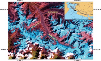
Fig. 1. Location of Gangotri Glacier in the Indian Himalaya. The tributary glaciers Kirti Bhamak and Chaturangi are also shown. This is one of the largest glaciers in the Central Himalaya.
Methodology
Landsat Thematic Mapper (TM) and Enhanced TM Plus (ETM+) imagery (30 m spatial resolution) was obtained for 2009 and 2010 (Table 1), during September and October, i.e. at the end of the melting season (http://earthexplorer.usgs.gov/). The post-monsoon months were chosen to ensure minimum cloud cover over the area of interest.
Table 1. Description of datasets used for analysis
Calculation of surface velocity fields
Surface velocities were calculated using sub-pixel correlation of the acquired images, using the freely available software Co-registration of Optically Sensed Images and Correlation (COSI-Corr), which is downloadable at http://www.tectonics.caltech.edu/. In this algorithm, two images are iteratively cross-correlated in the phase plane on sliding windows, to find the best possible correlation. A detailed description of the algorithm is given by Reference Leprince, Barbot, Ayoub and AvouacLeprince and others, (2007). After performing sub-pixel correlation, taking a sliding window of 32 × 32 pixels and a step size of two pixels we have three output images: a north/south displacement image, an east/west displacement image and a signal-to-noise ratio (SNR) image that describes the quality of correlation. All pixels that have SNR <0.9 and displacements >85 m are discarded. A vector field is generated from the two displacement images and is then overlaid on the image. After verifying the proper alignment of the displacement vectors along the length of the glacier, the Eulerian norm of the displacement images is calculated to find the magnitude of the resultant displacement. The difference in the time of acquisition between the two images isused to estimate the velocity field.
Estimation of depth
Ice thickness is estimated using the equation of laminar flow (Reference CuffeyCuffey and Paterson, 2010):
where U s and U b are surface and basal velocities, respectively. To date, no accurate estimate of basal velocity for Gangotri Glacier is available, so we assumed U b to be 25% of the surface velocity (Reference Swaroop, Raina and SangeswarSwaroop and others, 2003). Glen’s flow law exponent, n, is assumed to be 3, H is ice thickness and A is a creep parameter (which depends on temperature, fabric, grain size and impurity content and has a value of 3.24 × 10⁻²⁴ pa-3 s-1 for temperate glaciers; Reference CuffeyCuffey and Paterson, 2010). The basal stress is modeled as
Where ρ is the ice density, assigned a constant value of 900 kg m–3 (Reference Farinotti, Huss, Bauder, Funk and TrufferFarinotti and others, 2009a), g is acceleration due to gravity (9.8 m s–2) and f is a scale factor, i.e. the ratio between the driving stress and basal stress along a glacier, and has a range of [0.8, 1] for temperate glaciers. We use f = 0.8 (Reference Haeberli and HoelzleHaeberli and Hoelzle, 1995). Slope,α, is estimated from ASTER (Advanced Spaceborne Thermal Emission and Reflection Radiometer) DEM elevation contours, at 100 m intervals(http://reverb.echo.nasa.gov/reverb). This interval was chosen so the surface slope isaveraged over a reference distance that is about an order of magnitude larger than the local ice thickness (e.g.Reference Kamb and EchelmeyerKamb and Echelmeyer, 1986; Reference CuffeyCuffey and Paterson, 2010; Reference Linsbauer, Paul and HaeberliLinsbauer and others, 2012).

from which a depth for each area between successive 100 m contours is calculated. Finally, all these depths are plotted to provide an ice-thickness distribution for the entire glacier. The ice-thickness values are then smoothed using a 3 × 3 kernel, in order to remove any abrupt changes in spatial ice-thickness values.
Uncertainty and Sensitivity Analysis
The uncertainty in depth estimates is quantified by taking the natural logarithm of both sides of Eqn (3) and then differentiating:

Results
The surface velocities for Gangotri Glacier are shown in Figure 2. The velocities peak in the upper trunk section, reaching a value of ˜ 85 m a–1, and progressively decrease to <30 m a–1 in the lower reaches.
Fig. 2. Surface velocity field of Gangotri Glacier. The maximum velocities are found in the higher reaches and vary from 61 to 85 m a–1. The minimum velocities are found near the snout and at the glacier boundary, and vary from 5 to 15 m a–1. The two large determined by field investigation.
The ice-thickness distribution for Gangotri Glacier is shown in Figure 3a. Ice thickness attains a maximum of 540 m in the central part of the glacier’s main trunk. A thickness distribution range of 350–450 m was estimated in the upper reaches, while in the lower reaches the range was 150–200 m. At the snout the thickness was estimated to be in the range 40–65 m. Two cross-profiles at different positions on the glacier were plotted and are shown in Figure 3b.

Fig.3. (a) Ice-thickness distribution of Gangotri Glacier. Maximum ice thickness is ˜ 540 m in the central part of the main trunk. At the snout the thickness is estimated to be in the range 40–65 m. (b) The ice-thickness distribution along four cross-sectional profiles (1–4).
Validation
We validated the surface velocity field estimated over Gangotri Glacier using data collected during 1971 and 1972 (Reference Swaroop, Raina and SangeswarSwaroop and others, 2003). There are no direct ice-thickness measurements for Gangotri Glacier. However, there is an extensive set of direct measurements for both velocity field and ice thickness for Glacier de Corbassière, Swiss Alps, so we were able to validate our technique by estimating the velocity fields and ice-thickness distribution of the Alpine glacier using the same set of parameters as we had used for Gangotri Glacier.
The 1971 and 1972 field measurements of surface velocities (Reference Swaroop, Raina and SangeswarSwaroop and others, 2003) at the confluence of Kirti Bhamak Glacier and at Raktvarn Glacier (near the snout) are indicated by white dots in Figure 2. We assume that when the observations were made, the velocities were similar to those at present, meaning that the velocities we calculate here are comparable with those observed in the 1971 and 1972 field studies. Near Kirti Bhamak Glacier the difference (modelled values minus observed values) was ˜ 4 m a–1, and near Raktvarn Glacier it was 3 m a–1. The modelled outputs are thus slightly higher than those observed.
Surface velocity and ice-thickness distribution are calculated for Glacier de Corbassière (45.99038˚N, 7.26398˚E) using Landsat ETM+ imagery for 2004 and 2005 (Table 1) and were compared with observations (Glaciological Reports, 2009; Reference Gabbi, Farinotti, Bauder and MaurerGabbi and others, 2012). The velocity and ice-thickness profiles are presented in Figure 4.

Fig. 4. (a) Velocity field of Glacier de Corbassière. The maximum velocity varies from 60 to 84 m a–1. The minimum velocity varies from 3 to 10 m a–1. The white stars indicate sites where velocity was measured in the field (Glaciological Reports, 2009). (b) Ice-thickness distribution of Glacier de Corbassière (Reference Gabbi, Farinotti, Bauder and MaurerGabbi and others, 2012; Reference Linsbauer, Paul and HaeberliLinsbauer and others, 2012). Ground-penetrating radar soundings were made at nine cross sections, numbered 1–9. (c) Sensitivity of ice thickness to three values of basal velocity, expressed as per cent surface velocity: red – 34%, green – 30%, blue – 25%. The plots show the four cross sections of Glacier de Corbassière numbered 1–4 in (b). The ice thickness varies negligibly, even when basal velocity is varied by 10%.
The velocity profiles of Glaciological Reports, (2009) were compared at the sites indicated by white stars in Figure 4a. The absolute error for each point was found to be <6 m a–1 for all but one of the seven points.
The ice-thickness profile was estimated using the same approach, and was compared with that estimated by Reference Gabbi, Farinotti, Bauder and MaurerGabbi and others, (2012) and Reference Linsbauer, Paul and HaeberliLinsbauer and others, (2012). Ground-penetrating radar (GPR) profiles were available for four cross sections, numbered 1–9 in Figure 4b. Since GPR soundings give point-to-point measurements, while our thickness profile is over an area of 3600 km2, differences between the means of observed thickness values and modelled thickness values were computed. The relative differences were 5%, 0%, 12.3%, 28.9%, 17%, 15%, 7%, 9.9% and 5% for cross sections 1, 2, 3, 4, 5, 6, 7, 8 and 9, respectively. Except for cross sections 5 and 6, the modelled values were slightly higher than those observed. The total volume of stored ice from our investigation is ˜ 1.8 ± 0.5 km3. This compares well with the estimates of Reference Gabbi, Farinotti, Bauder and MaurerGabbi and others, (2012) and Farinotti and others (2009b), who suggest values of 1.36 ± 0.07 and 1.96 km3, respectively.
Uncertainty and Sensitivity Analysis
Uncertainties in the estimation of ice thickness depend on: (1) uncertainty in velocity estimates; (2) uncertainty in the creep parameter, A; (3) uncertainty in the shape factor, f; (4) uncertainty in the density of ice; and (5) uncertainty in estimation of slope angle, α.
There are two sources of uncertainty in velocity estimates. (1) The uncertainty introduced due to orthorectification errors can be determined by examining the displacements over ice-free ground (where the displacements may be assumed to be zero). In our analyses, all the pixels that represented displacement over ice-free ground showed a root-mean-square displacement of 5–9 m, with a maximum of 12 m. (2) Uncertainty is also introduced by decorrelation caused by the presence of cloud cover over the glaciers. For this reason, we only used images with minimal cloud cover over the region of interest. Seasonal snow cover also biases the velocity measurements by masking the features present on the glacier surface, due to which the algorithm fails. Therefore only images at the end of the melting season were analysed. Decorrelation can also occur at the snout, due to melting or changes in land surface characteristics caused by landslides.
In order to quantify the total uncertainty (for a particular value of basal velocity, i.e. 25% of surface velocity) in volume estimation using Eqn (4), we fix the values for dU s,df, dρ, d(sin α)/(sin α) and dA. The reason we do not consider variation in basal velocity can be seen from Figure 4c, which shows the variation of ice-thickness estimates for three values of basal velocity. The ice thickness varies by a very small magnitude for a given range of basal velocities (expressed as per cent of surface velocity).
The value of dU s was fixed as 3.5 m a–1, which is the average of the differences (between observed and modelled outputs) obtained at the two sites by Reference Swaroop, Raina and SangeswarSwaroop and others, (2003), and df was set to 0.1. In the literature (e.g. Reference Hubbard, Blatter, Nienow, Mair and HubbardHubbard and others, 1998; Reference GudmundssonGudmundsson, 1999; Reference Farinotti, Huss, Bauder, Funk and TrufferFarinotti and others, 2009a) A is set to 2.4 × 10⁻²⁴ Pa–3 s–1. We set dA to be the difference between the value assigned by us and 2.4 × 10⁻²⁴ Pa–3 s–1. To estimate the uncertainty in slope angle over a region, the vertical accuracy of the DEM must be known. The potential uncertainty in the ASTER DEM for the Himalayan region is 11 m (Fujita and others, 2004). Therefore, the term d(sin α)/(sin α) has a value of 0.09. Variation in ice density, ρ, over the depth of the glacier is not known. We assume relative uncertainties of 10%, and take dρ as 90 kg m–3.
Substituting these values into Eqn (4), we find the maximum relative error in the volume measurement for Gangotri Glacier is ± 18.1% (assuming that the parameters vary independently and randomly)
Conclusions
We have estimated the ice thickness for Gangotri Glacier from surface velocities and slope, using the flow law of ice. The velocities varied from 14 to 85 ma-1 in the lower reaches. The ice thickness attained a maximum value of ˜ 540 m; a range of 350–450 m was found in the upper reaches; in the lower reaches the range was 150–200 m and at the snout it was 50–65 m. The total volume of Gangotri Glacier is ˜ 23.2 ± 4.2 km3 (18% uncertainty). These analyses show that the method has the potential to improve estimates of the ice-thickness distribution of glaciers where mass-balance data are not available, as is the case for most large Himalayan glaciers. This will help in assessing the sustainability of Himalayan glaciers.
Acknowledgements
We thank the Divecha Centre for Climate Change for providing laboratory resources. We also thank Sébastien Leprince for vital suggestions during the calculation of displacement maps over the glacier. We are grateful to the US Geological Survey for its free data policy, allowing us to use Landsat TM/ETM+ imagery. We thank Helgi Björnsson for valuable insights into glacier dynamics, which helped us to carry out this analysis.


