2.1. The dynamical equations

In past studies of fast-wave averaging (e.g. Embid & Majda Reference Embid and Majda1996), the dry Boussinesq equations have been investigated. Here, instead, moist Boussinesq equations are investigated, in order to assess the impact of phase changes between water vapour and liquid water, following Zhang et al. (Reference Zhang, Smith and Stechmann2021). The governing equations are

(2.1)\begin{gather} \dfrac{\textrm{D}\boldsymbol{u}}{\textrm{D}t} + f \hat{z} \times \boldsymbol{u} ={-}\boldsymbol{\nabla}\phi + \hat{z}b, \end{gather}

(2.2)\begin{gather} \boldsymbol{\nabla} \boldsymbol{\cdot} \boldsymbol{u}=0, \end{gather}

(2.3)\begin{gather} \dfrac{\textrm{D}\theta}{\textrm{D}t} + w\dfrac{\textrm{d}\tilde{\theta}}{\textrm{d}z} = \dfrac{L_v}{c_p}C, \end{gather}

(2.4)\begin{gather} \dfrac{\textrm{D} q_v}{\textrm{D}t} + w\dfrac{\textrm{d}\tilde{q}_v}{\textrm{d}z} ={-}C, \end{gather}

(2.5)\begin{gather} \dfrac{\textrm{D} q_l}{\textrm{D}t} = C. \end{gather}

Here, $\boldsymbol {u} = (\boldsymbol {u}_h,w)$ is the three-dimensional velocity with horizontal components $\boldsymbol {u}_h=(u,v)$ and vertical component $w$. The material derivative is defined as ${\textrm {D}}/{\textrm {D}t} = \partial _t + \boldsymbol {u} \boldsymbol {\cdot } \boldsymbol {\nabla }$, where the three-dimensional gradient operator is $\boldsymbol {\nabla }=(\partial _x,\partial _y,\partial _z)$. The conservation of momentum equation is in (2.1), including the Coriolis term, $f\hat {z} \times \boldsymbol {u} = (-fv,fu,0)^{\intercal }$, which represents the effects of rotation. The unit vector in the vertical direction is $\hat {z}=(0,0,1)$ and the pressure-like variable is $\phi$. A constant Coriolis parameter $f$ is used here.

The buoyancy term $\hat {z}b$ in (2.1) is defined as

(2.6)\begin{equation} b = g\left( \frac{\theta}{\theta_0} + R_{vd}q_v -q_l \right), \end{equation}

where $g=9.8\ \textrm {m}\,\textrm {s}^{-2}$ is the gravitational acceleration, $\theta _0=300\,\textrm {K}$ is a reference background value of potential temperature, and $R_{vd}=(R_v/R_d) - 1\approx 0.61$, where $R_d$ is the gas constant for dry air and $R_v$ is the gas constant for water vapour.

Three thermodynamic variables are evolving in time according to (2.3)–(2.5). The potential temperature is $\theta$, the water vapour mixing ratio is $q_v$ and the liquid water mixing ratio is $q_l$, and all three of these quantities are anomalies. More specifically, the thermodynamic quantities have been decomposed as $\theta ^{tot}(\boldsymbol {x},t)=\tilde {\theta }(z)+\theta (\boldsymbol {x},t)$ and $q_v^{tot}(\boldsymbol {x},t)=\tilde {q}_v(z)+q_v(\boldsymbol {x},t)$, so that the total quantity is written as the sum of a prescribed, background function of altitude $z$ and an anomaly. Note that the background state is chosen to be cloud-free, so $\tilde {q}_l=0$ and $q_l^{tot}=q_l$. Furthermore, the background gradients $d\tilde {\theta }/\textrm {d}z$ and $\textrm {d}\tilde {q}_v/\textrm {d}z$ are chosen to be constants, for simplicity, which helps to render (2.1)–(2.5) a constant-coefficient system within each phase, and a piecewise-constant-coefficient system overall, since some coefficients change their values due to phase changes.

Phase changes enter into (2.3)–(2.5) via $C$, which represents the rate of condensation and evaporation. Condensation occurs for $C>0$ and represents a phase transition from vapour to liquid, and evaporation occurs for $C<0$ and represents a phase transition from liquid to vapour. The definition of $C$ is

(2.7)\begin{equation} C = \left\{ \begin{array}{@{}ll} 0, & \text{ if } q_v^{tot} < q_{vs}^{tot},\\ -\dfrac{\textrm{D}q^{tot}_{vs}}{\textrm{D}t}, & \text{ if } q_v^{tot} = q_{vs}^{tot} , \end{array} \right. \end{equation}

where the threshold $q_{vs}^{tot}$ is the saturation water vapour mixing ratio. In other words, in (2.7), if the vapour is below the threshold, then neither condensation nor evaporation occurs; and if the vapour reaches the threshold, then condensation or evaporation will occur (so $C\neq 0$) and is defined so as to maintain the vapour value at its threshold value: $q_v^{tot}=q_{vs}^{tot}$. Indeed, from inserting (2.7) into (2.4), one can see that, if $q_v^{tot}=q_{vs}^{tot}$, then $Dq_v^{tot}/Dt=Dq_{vs}^{tot}/Dt$. To close the evolution, the threshold $q_{vs}^{tot}$ must be specified. In comprehensive treatments of moist thermodynamics, one would define $q_{vs}^{tot}$ to be a function of temperature and pressure, according to the Clausius–Clapeyron equation (e.g. Rogers & Yau Reference Rogers and Yau1989; Grabowski & Smolarkiewicz Reference Grabowski and Smolarkiewicz1996; Klein & Majda Reference Klein and Majda2006). Here, as a more simplistic treatment, it is defined as a function of height $z$ alone, as $q_{vs}^{tot}(z)$. Such a treatment arises from assuming that temperature $T^{tot}$ and pressure $p^{tot}$ are nearly equal to their background values $\tilde {T}(z)$ and $\tilde {p}(z)$, in which case $q_{vs}^{tot}(T^{tot},p^{tot})\approx q_{vs}^{tot}(\tilde {T}(z),\tilde {p}(z))$ as a first approximation (e.g. Hernandez-Duenas et al. Reference Hernandez-Duenas, Majda, Smith and Stechmann2013). In this case, with $q_{vs}^{tot}=q_{vs}^{tot}(z)$, (2.7) becomes

(2.8)\begin{equation} C = \left\{ \begin{array}{@{}ll} 0, & \text{ if } q_v^{tot} < q_{vs}^{tot},\\ -w\dfrac{\textrm{d}q^{tot}_{vs}(z)}{\textrm{d}z}, & \text{ if } q_v^{tot} = q_{vs}^{tot} . \end{array} \right. \end{equation}

In (2.8), the saturation value $q_{vs}^{tot}(z)$ is usually decreasing as altitude increases, so that $\textrm {d}q_{vs}^{tot}(z)/\textrm {d}z<0$. As a result, one can see from (2.8) that, within a cloud, upward vertical velocity ($w>0$) is associated with condensation ($C>0$) and cloud formation, and, on the other hand, downward vertical velocity ($w<0$) is associated with evaporation of cloud water ($C<0$). Furthermore, condensation is associated with heating in (2.3), and evaporation is associated with cooling. The latent heat of vaporization is a constant parameter, $L_v=2.5\times 10^{6}\ \textrm {J}\,\textrm {kg}^{-1}$, and the specific heat is also a constant parameter, $c_p=10^3\ \textrm {J}\,\textrm {kg}^{-1}\,\textrm {K}^{-1}$. Note that the present version of $C$ uses instantaneous saturation adjustment, whereby the water vapour $q_v$ is instantaneously adjusted to maintain the saturation constraint $q_t=q_{vs}$, whereas this adjustment time scale is finite (but very small) in nature (e.g. Grabowski & Morrison Reference Grabowski and Morrison2008).

The moist Boussinesq system in (2.1)–(2.8) is used as an idealized model of atmospheric dynamics with phase changes. Models like (2.1)–(2.8) have also been used for many purposes and with varying degrees of idealization (e.g. Kuo Reference Kuo1961; Sommeria Reference Sommeria1976; Bretherton Reference Bretherton1987; Cuijpers & Duynkerke Reference Cuijpers and Duynkerke1993; Spyksma et al. Reference Spyksma, Bartello and Yau2006; Stechmann & Stevens Reference Stechmann and Stevens2010; Pauluis & Schumacher Reference Pauluis and Schumacher2010). Here, the moist Boussinesq system is intended to be used as an extension of dry Boussinesq models that have previously been studied in geophysical fluid dynamics (e.g. Embid & Majda (Reference Embid and Majda1996), Majda (Reference Majda2003), Hernandez-Duenas, Smith & Stechmann (Reference Hernandez-Duenas, Smith and Stechmann2014) and other references described in § 1). The moist system in (2.1)–(2.8) will reduce to the dry Boussinesq system if water vapour $q_v$, liquid water $q_l$ and condensation/evaporation $C$ are neglected.

While clouds are included in (2.1)–(2.8), they are included in their most basic form. Other aspects, such as rain and ice, are not considered here, in order to put emphasis on the basic vapour–liquid phase change, which already introduces additional non-trivial behaviour. Therefore, in comparing (2.1)–(2.8) with the set-up of Zhang et al. (Reference Zhang, Smith and Stechmann2021), one distinction is that the fall velocity of rain, $V_T$, has been set to zero here, and it is then cloud liquid water $q_l$ that appears here instead of rain water $q_r$. Nevertheless, while many complicated cloud processes have been neglected here, the system in (2.1)–(2.8) provides the starting point for extensions that include rainfall and other complexities (e.g. Grabowski & Smolarkiewicz Reference Grabowski and Smolarkiewicz1996; Klein & Majda Reference Klein and Majda2006).

For use in the remainder of the paper, it is convenient to rewrite (2.1)–(2.8) in terms of a different set of thermodynamic variables that are conserved. In particular, define the anomalies of equivalent potential temperature, $\theta _e$, and total water mixing ratio, $q_t$, as

(2.9)\begin{gather} \theta_e = \theta+\frac{L_v}{c_p}q_v, \end{gather}

(2.10)\begin{gather}q_t = q_v + q_l. \end{gather}

The evolution equations of $\theta _e$ and $q_t$ can be found by taking appropriate linear combinations of (2.3)–(2.5), and they take the form

(2.11)\begin{gather} \dfrac{\textrm{D}\theta_e}{\textrm{D}t} + w\dfrac{\textrm{d}\tilde{\theta}_e}{\textrm{d}z} = 0, \end{gather}

(2.12)\begin{gather}\dfrac{\textrm{D} q_t}{\textrm{D}t} + w\dfrac{\textrm{d}\tilde{q}_t}{\textrm{d}z} = 0, \end{gather}

where the background states are defined, similar to (2.9)–(2.10), as $\tilde {\theta }_e(z)=\tilde {\theta }(z)+(L_v/c_p)\tilde {q}_v(z)$ and $\tilde {q}_t(z)=\tilde {q}_v(z)+\tilde {q}_l(z)=\tilde {q}_v(z)$. The important feature of (2.11)–(2.12) is that the source term of condensation/evaporation, $C$, has been eliminated. As a result, (2.11)–(2.12) show that $\theta _e+\tilde {\theta }_e(z)$ and $q_t+\tilde {q}_t(z)$ are conserved along fluid parcel trajectories. Physically, the equivalent potential temperature is conserved because losses of water vapour $q_v$ are compensated by gains in heat $\theta$, as indicated by the definition in (2.9); and the total water mixing ratio, $q_t=q_v+q_l$, is conserved because losses of water vapour $q_v$ are compensated by gains in liquid water $q_l$.

To complete the rewriting, the buoyancy $b$ from (2.6) must also be rewritten in terms of $\theta _e$ and $q_t$. To do so, the following transformation is used:

(2.13)\begin{gather} \theta = \theta_e - \frac{L_v}{c_p}\min(q_t,q_{vs}), \end{gather}

(2.14)\begin{gather}q_v = \min(q_t,q_{vs}), \end{gather}

(2.15)\begin{gather}q_l = \max(0,q_t-q_{vs}), \end{gather}

which is the reverse of the transformation in (2.9)–(2.10). Note that an anomalous $q_{vs}$ has been introduced, via a decomposition $q_{vs}^{tot}(z)=\tilde {q}_{vs}(z)+q_{vs}$; and the background state is chosen to be $\tilde {q}_{vs}=\tilde {q}_t$ so that the surplus water above saturation, $q_t^{tot}-q_{vs}^{tot}$, can be written equivalently as $q_t-q_{vs}$ and retains essentially the same form when written in terms of anomalies. The anomaly $q_{vs}$ will be a constant parameter here. By inserting (2.13)–(2.15) into the definition of buoyancy $b$ in (2.6), one arrives at

(2.16)\begin{equation} b = g\left\{ \begin{array}{@{}ll} \displaystyle\dfrac{\theta_e}{\theta_0} + \left(R_{vd}-\displaystyle\dfrac{L_v}{c_p\theta_0}\right)q_t & \text{if}\ q_t< q_{vs},\\ \displaystyle\dfrac{\theta_e}{\theta_0} + \left(R_{vd}-\displaystyle\dfrac{L_v}{c_p\theta_0}\right)q_{vs} - (q_t-q_{vs}) & \text{if}\ q_t\ge q_{vs}, \end{array} \right. \end{equation}

which is the desired expression for buoyancy $b$ in terms of the variables $\theta _e$ and $q_t$.

To summarize the rewriting in terms of conserved variables, the original system (2.1)–(2.8) can be written in alternative form as

(2.17)\begin{gather} \dfrac{\textrm{D}\boldsymbol{u}}{\textrm{D}t} + f \hat{z} \times \boldsymbol{u} ={-}\boldsymbol{\nabla}\phi + \hat{z}b, \end{gather}

(2.18)\begin{gather} \boldsymbol{\nabla} \boldsymbol{\cdot} \boldsymbol{u}=0, \end{gather}

(2.19)\begin{gather} \dfrac{\textrm{D}\theta_e}{\textrm{D}t} + w\dfrac{\textrm{d}\tilde{\theta}_e}{\textrm{d}z} = 0, \end{gather}

(2.20)\begin{gather} \dfrac{\textrm{D} q_t}{\textrm{D}t} + w\dfrac{\textrm{d}\tilde{q}_t}{\textrm{d}z} = 0, \end{gather}

along with the definition of buoyancy $b$ from (2.16). The formulation in (2.16)–(2.20) will be used in the remainder of the paper.

While the $(\theta ,q_v,q_l)$ formulation in (2.1)–(2.8) is helpful for seeing the connection with a dry system, the $(\theta _e,q_t)$ formulation in (2.16)–(2.20) is helpful for another reason that is central to the goals of the present paper: for defining the slow modes of the system. The slow modes will be defined below in § 2.2.

As the next two steps of the model specification, we first create a non-dimensional system, and, second, identify the small parameter $\epsilon$. To non-dimensionalize the system, reference values are chosen for all variables as in table 1. For instance, the non-dimensional velocity $u^*$ is defined as $u^*=u/U$, by dividing the dimensional $u$ by the reference value $U$. In terms of non-dimensional quantities, the main system in (2.16)–(2.20) becomes, after dropping the superscript $*$ to ease notation,

(2.21)\begin{gather} \dfrac{\textrm{D}_h\boldsymbol{u}_h}{\textrm{D}t}+w\dfrac{\partial \boldsymbol{u}_h}{\partial z}+Ro^{{-}1}\boldsymbol{u}_h^{\bot}+Eu\boldsymbol{\nabla}_h\phi=0, \end{gather}

(2.22)\begin{gather} A^2\left(\dfrac{\textrm{D}_hw}{\textrm{D}t}+w\dfrac{\partial w}{\partial z}\right)+Eu\dfrac{\partial\phi}{\partial z}-\varGamma A^2 b=0, \end{gather}

(2.23)\begin{gather} \boldsymbol{\nabla}_h\boldsymbol{\cdot} \boldsymbol{u}_h+\dfrac{\partial w}{\partial z}=0, \end{gather}

(2.24)\begin{gather} \dfrac{\textrm{D}_h\theta_e}{\textrm{D}t}+w\dfrac{\partial \theta_e}{\partial z}+{Fr_1}^{{-}2}(\varGamma A^2)^{{-}1}w=0, \end{gather}

(2.25)\begin{gather} \dfrac{\textrm{D}_h q_t}{\textrm{D}t}+w\dfrac{\partial q_t}{\partial z}-{Fr_2}^{{-}2}(\varGamma A^2)^{{-}1}w=0 \end{gather}

and the non-dimensional buoyancy definition,

(2.26)\begin{equation} b = \left\{ \begin{array}{@{}ll} \theta_e + \left(R_{vd}\displaystyle\dfrac{c_p\theta_0}{L_v}-1\right)q_t & \text{if}\ q_t< q_{vs},\\ \theta_e + \left(R_{vd}\displaystyle\dfrac{c_p\theta_0}{L_v}-1\right)q_{vs} - \displaystyle\dfrac{c_p\theta_0}{L_v}(q_t-q_{vs}) & \text{if}\ q_t\ge q_{vs}. \end{array} \right. \end{equation}

Note that the material derivative has been split into its horizontal part, $D_h/Dt=\partial _t+\boldsymbol {u}_h\boldsymbol {\cdot }\boldsymbol {\nabla }_h$, and vertical part, $w\partial _z$, where $\boldsymbol {\nabla }_h=(\partial _x,\partial _y)$ is the horizontal part of the gradient operator. In the non-dimensional equations above, the non-dimensional parameters include the Rossby number $Ro$, Euler number $Eu$, aspect ratio $A$ and buoyancy parameter $\varGamma$, all of which are defined by analogy with the dry Boussinesq parameters (e.g. Majda Reference Majda2003) and are defined here in table 2. A new parameter arises in (2.26) due to moisture: the thermodynamic parameter ratio, $c_p\theta _0/L_v\approx 0.1$.

Table 1. Reference scales used for each variable to create non-dimensional equations.

Table 2. Non-dimensional parameters.

Two other parameters, $Fr_1$ and $Fr_2$, also appear in (2.21)–(2.26), and some further explanation is required to relate them to traditional parameters of the dry Boussinesq equations. The two parameters $Fr_1$ and $Fr_2$ are similar to Froude numbers, and two of them appear here because the moist system involves two thermodynamic variables ($\theta _e$ and $q_t$), as opposed to the dry case with one Froude number and one thermodynamic variable ($\theta$). The definitions here are

(2.27a,b)\begin{equation} Fr_1=\frac{U}{N_1 H}, \quad Fr_2=\frac{U}{N_2 H}, \end{equation}

where $H$ is the reference height, $U$ is the reference horizontal velocity and

(2.28a)\begin{gather} {N_1}^2 = \dfrac{g}{\theta_0} \dfrac{\textrm{d} \tilde{\theta}_e }{\textrm{d}z} = \dfrac{g}{\theta_0} \dfrac{\textrm{d}}{\textrm{d}z} \left(\tilde{\theta} + \dfrac{L_v}{c_p}\tilde{q}_{v}\right), \end{gather}

(2.28b)\begin{gather}{N_2}^2 ={-} \dfrac{g}{\theta_0} \dfrac{L_v}{c_p} \dfrac{\textrm{d}\tilde{q}_t }{\textrm{d}z} ={-} \dfrac{g}{\theta_0} \dfrac{L_v}{c_p} \dfrac{\textrm{d}\tilde{q}_v }{\textrm{d}z}. \end{gather}

The parameters $N_1$ and $N_2$ are constants because the background gradients, $\textrm {d}\tilde {\theta }_e/\textrm {d}z$ and $\textrm {d}\tilde {q}_t/\textrm {d}z$, have been chosen to be constants here, as is typical for a Boussinesq system. The notation $N$ is used for $N_1$ and $N_2$ in analogy with the notation for the buoyancy frequency of a dry system, $N^2=(g/\theta _0)\,\textrm {d}\tilde {\theta }/\textrm {d}z$. For the moist system here, the two buoyancy frequencies are

(2.29a,b)\begin{equation} {N_u}^2 = \dfrac{g}{\theta_0} \dfrac{\textrm{d} \tilde{\theta} }{\textrm{d}z}, \quad {N_s}^2 = \dfrac{g}{\theta_0} \dfrac{\textrm{d} \tilde{\theta}_e }{\textrm{d}z}, \end{equation}

and they involve $\theta$ and $\theta _e$, respectively, because, from (2.26), the non-dimensional buoyancy is $b\approx \theta _e-q_t=\theta$ in unsaturated regions and $b\approx \theta _e-q_{vs}=\theta _e-const.$ in saturated regions. These approximations neglect terms in (2.26) that are proportional to $c_p\theta _0/L_v\approx 0.1$, to simplify the expressions for clarity. The buoyancy frequency, or Brunt–Väisälä frequency, describes the frequency of buoyancy oscillations, and one can compute it in either the unsaturated or saturated phase (Durran & Klemp Reference Durran and Klemp1982a,Reference Durran and Klempb). More complete expressions for the present model's $N_u$ and $N_s$ are derived by Smith & Stechmann (Reference Smith and Stechmann2017) in their appendix without neglecting terms proportional to $c_p\theta _0/L_v\approx 0.1$. Associated with the buoyancy frequencies $N_u$ and $N_s$ are two Froude numbers,

(2.30a,b)\begin{equation} Fr_u=\frac{U}{N_u H}, \quad Fr_s=\frac{U}{N_s H}. \end{equation}

Finally, then, by comparing (2.28) and (2.29a,b), one can see that the parameter sets $(N_1,N_2)$ and $(N_u,N_s)$ are related as

(2.31a,b)\begin{equation} {N_u}^{2} = {N_1}^2 + {N_2}^2, \quad N_s = N_1, \end{equation}

and therefore the parameter sets $(Fr_1,Fr_2)$ and $(Fr_u,Fr_s)$ are related as

(2.32a,b)\begin{equation} Fr_u^{{-}2} = Fr_1^{{-}2} + Fr_2^{{-}2}, \quad Fr_s^{{-}1} = Fr_1^{{-}1}. \end{equation}

As a result of these relationships, one can work with either $(N_1,N_2)$ and $(Fr_1,Fr_2)$ on the one hand, or with $(N_u,N_s)$ and $(Fr_u,Fr_s)$ on the other hand. Here, $(N_1,N_2)$ and $(Fr_1,Fr_2)$ will be used, since they appear directly in the equations of motion in (2.21)–(2.26) when using the variables $\theta _e$ and $q_t$.

Parameter values are chosen to represent rapid rotation (small Rossby number) and strong stratification (small Froude number). The Rossby number is defined to be the small parameter $\epsilon$,

(2.33)\begin{equation} Ro=\epsilon, \end{equation}

and the other parameters are related to $Ro$ in a distinguished limit as

(2.34a–c)\begin{gather} Fr_1=Ro\dfrac{L}{L_{d_1}} = O{(\epsilon)} , \quad {Fr_2}=Ro\dfrac{L}{L_{d_2}} = O{(\epsilon)} , \quad \varGamma A^2={Fr_1}^{{-}1 } = O(\epsilon^{{-}1}) , \end{gather}

(2.35a,b)\begin{gather}Eu^{{-}1}=Ro=\epsilon , \quad \dfrac{c_p \theta_0}{L_v} = C_{cl}Ro = O(\epsilon), \end{gather}

where $L_{d_1}$ and $L_{d_2}$ are similar to Rossby radii of deformation and are defined as

(2.36a,b)\begin{equation} L_{d_1}=\dfrac{N_1H}{f}, \quad L_{d_2}=\dfrac{N_2H}{f}. \end{equation}

With these parameter relationships, the non-dimensional equations from (2.21)–(2.26) become

(2.37)\begin{gather} \dfrac{\textrm{D}_h\boldsymbol{u}_h}{\textrm{D}t}+w\dfrac{\partial \boldsymbol{u}_h}{\partial z}+\epsilon^{{-}1}\boldsymbol{u}_h^{\bot}+\epsilon^{{-}1}\boldsymbol{\nabla}_h\phi=0, \end{gather}

(2.38)\begin{gather} A^2\left(\dfrac{\textrm{D}_hw}{\textrm{D}t}+w\dfrac{\partial w}{\partial z}\right)+\epsilon^{{-}1}\dfrac{\partial\phi}{\partial z}-\epsilon^{{-}1}\frac{L_{d_1}}{L} b=0, \end{gather}

(2.39)\begin{gather} \boldsymbol{\nabla}_h\boldsymbol{\cdot} \boldsymbol{u}_h+\dfrac{\partial w}{\partial z}=0, \end{gather}

(2.40)\begin{gather} \dfrac{\textrm{D}_h\theta_e}{\textrm{D}t}+w\dfrac{\partial \theta_e}{\partial z}+\epsilon^{{-}1}\frac{L_{d_1}}{L}w=0, \end{gather}

(2.41)\begin{gather} \dfrac{\textrm{D}_h q_t}{\textrm{D}t}+w\dfrac{\partial q_t}{\partial z}-\epsilon^{{-}1}\frac{L_{d_2}}{L}\frac{L_{d_2}}{L_{d_1}}w=0 \end{gather}

and the non-dimensional buoyancy definition,

(2.42)\begin{equation} b = \left\{ \begin{array}{@{}ll} \theta_e + \left(\epsilon R_{vd}C_{cl}-1\right)q_t & \text{if}\ q_t< q_{vs},\\ \theta_e + \left(\epsilon R_{vd}C_{cl}-1\right)q_{vs} - \epsilon C_{cl}(q_t-q_{vs}) & \text{if}\ q_t\ge q_{vs}. \end{array} \right. \end{equation}

In arriving at (2.37)–(2.42), the scaling scenario is similar to dry fast-wave averaging (e.g. Embid & Majda Reference Embid and Majda1996), with extensions to the present case with moisture, following Smith & Stechmann (Reference Smith and Stechmann2017), and discussed further below. While one could proceed with (2.37)–(2.42), the analysis would be complicated by the many $O(1)$ constants that appear: $A,L/L_{d_1},L/L_{d_2},R_{vd}$ and $C_{cl}$. To simplify the notation in what follows, these $O(1)$ constants will be set equal to unity, which leads to

(2.43)\begin{gather} \dfrac{\textrm{D}_h\boldsymbol{u}_h}{\textrm{D}t}+w\dfrac{\partial \boldsymbol{u}_h}{\partial z}+\epsilon^{{-}1}\boldsymbol{u}_h^{\bot}+\epsilon^{{-}1}\boldsymbol{\nabla}_h\phi=0, \end{gather}

(2.44)\begin{gather} \dfrac{\textrm{D}_hw}{\textrm{D}t}+w\dfrac{\partial w}{\partial z}+\epsilon^{{-}1}\dfrac{\partial\phi}{\partial z}-\epsilon^{{-}1} b=0, \end{gather}

(2.45)\begin{gather} \boldsymbol{\nabla}_h\boldsymbol{\cdot} \boldsymbol{u}_h+\dfrac{\partial w}{\partial z}=0, \end{gather}

(2.46)\begin{gather} \dfrac{\textrm{D}_h\theta_e}{\textrm{D}t}+w\dfrac{\partial \theta_e}{\partial z}+\epsilon^{{-}1}w=0, \end{gather}

(2.47)\begin{gather} \dfrac{\textrm{D}_h q_t}{\textrm{D}t}+w\dfrac{\partial q_t}{\partial z}-\epsilon^{{-}1}w=0 \end{gather}

and the non-dimensional buoyancy definition,

(2.48)\begin{equation} b = \left\{ \begin{array}{@{}ll} \theta_e + \left(\epsilon -1\right)q_t & \text{if}\ q_t< q_{vs},\\ \theta_e + \left(\epsilon -1\right)q_{vs} - \epsilon (q_t-q_{vs}) & \text{if}\ q_t\ge q_{vs}. \end{array} \right. \end{equation}

where each term in (2.43)–(2.48) now has a coefficient that is either unity or $\epsilon$. This completes the specification of the model, in non-dimensional units, in (2.43)–(2.48), for use in the remainder of the manuscript.

To provide some additional physical context, we describe how the scaling regime used here is reminiscent of the midlatitude atmosphere on synoptic scales, if a value of $\epsilon \approx 0.1$ is used (e.g. Majda Reference Majda2003; Vallis Reference Vallis2006; Smith & Stechmann Reference Smith and Stechmann2017). For instance, one can arrive at $Ro,Fr_1,Fr_2$ values of approximately 0.1 in the following way. For $f=10^{-4}\ \textrm {s}^{-1}$, $L=10^6\ \textrm {m}$ and $U=10\ \textrm {m}\,\textrm {s}^{-1}$, the Rossby number is $Ro=0.1$; and for $\textrm {d}\tilde {\theta }/\textrm {d}z=3\ \textrm {K}\,\textrm {km}^{-1}$, $d\tilde {q}_v/dz=-0.6$ g kg$^{-1}$ km$^{-1}$ and $H=10^{4}$ m, one has $N_1^2\approx N_2^2$ and $Fr_1\approx Fr_2\approx 0.14$. In this case, the buoyancy frequencies are related as $N_u^2\approx 2N_s^2$, consistent with a moist (or saturated) buoyancy frequency that is lower frequency than the dry (or unsaturated) buoyancy frequency. Hence the scaling choice of $Fr_1=Fr_2$ is physically realistic in this sense. One scaling choice that deviates slightly from established physical values is the choice of $R_{vd}=1$, where $R_{vd}$ is a parameter that is related to the gas constants for water vapour and dry air, as described above, and its value in reality is 0.61; nevertheless, this term does not arise at leading order in (2.42) and is not a central aspect of the analysis here. Also, the aspect ratio has been chosen to be $A=1$ here, which differs from typical values for the midlatitude atmosphere on synoptic scales (e.g. Vallis Reference Vallis2006; Smith & Stechmann Reference Smith and Stechmann2017), but is consistent with earlier studies of fast-wave averaging in the dry case (e.g. Embid & Majda Reference Embid and Majda1996; Majda Reference Majda2003). Indeed, in summarizing the parameter choices, the present study is an investigation of fast-wave averaging, and it uses parameter values that are consistent with and motivated by the midlatitude atmosphere on synoptic scales, but it is an idealized set-up, as in earlier fast-wave averaging studies (e.g. Embid & Majda Reference Embid and Majda1996; Majda Reference Majda2003). As such, the present paper will consider a variety of different $\epsilon$ values as $\epsilon$ tends toward zero.

For later use, we note that the buoyancy $b$ in (2.48) can be written in an alternative form as

(2.49)\begin{equation} b = H_ub_u + H_sb_s, \end{equation}

where $H_u$ and $H_s$ are Heaviside functions that indicate the unsaturated and saturated phases, respectively:

(2.50a,b)\begin{equation} H_u = \left\{ \begin{array}{@{}ll} 1 & \text{for } q_t < {q_{vs}},\\ 0 & \text{for } q_t \geq q_{vs}, \end{array}\right. \quad \text{and}\quad H_s = 1 - H_u. \end{equation}

In (2.49), the expressions for the unsaturated buoyancy $b_u$ and the saturated buoyancy $b_s$ are given by

(2.51a,b)\begin{equation} b_u = \theta_e + (\epsilon - 1)q_t, \quad b_s = \theta_e + (\epsilon - 1)q_{vs} - \epsilon (q_t-q_{vs}), \end{equation}

which follow from comparison with the earlier expression for $b$ in (2.48). By using the Heaviside functions, the expression in (2.49) can be used to describe the buoyancy succinctly, and the Heaviside functions provide a clear indication that the form of the buoyancy will change in different phases.

2.2. Slow variables

The premise of fast-wave averaging depends on separation of slowly varying and fast-wave components of the system. On the one hand, when fast waves evolve in time, they are influenced by the $\epsilon ^{-1}$ terms in the moist Boussinesq system in (2.43)–(2.48). Physically, the $\epsilon ^{-1}$ terms represent the effects of rapid rotation and strong stratification, which can cause fast-wave oscillations. On the other hand, slow variables will have evolution equations that are not influenced by the $\epsilon ^{-1}$ terms.

Keeping these features in mind, we here present an algebraic construction of the slow variables (a derivation using operator analysis may be found in Zhang et al. (Reference Zhang, Smith and Stechmann2021)). The construction draws upon foundations from previous literature regarding dry and moist dynamics, in particular, to identify potential vorticity variables (see e.g. Majda (Reference Majda2003), Marquet (Reference Marquet2014), Wetzel et al. (Reference Wetzel, Smith, Stechmann, Martin and Zhang2020) and references therein). In addition, for the moist system described in § 2.1, a second slow variable has been found and named $M$ (Smith & Stechmann Reference Smith and Stechmann2017; Wetzel et al. Reference Wetzel, Smith, Stechmann and Martin2019b, Reference Wetzel, Smith, Stechmann, Martin and Zhang2020).

First, to define the slow variable $M$, we follow the intuition mentioned above: the goal is to construct a new quantity whose evolution equation does not involve any $\epsilon ^{-1}$ terms. We look into the evolution equations for $\theta _e$ and $q_t$ in (2.46)–(2.47). In particular, while the $\theta _e$ evolution in (2.46) involves an $\epsilon ^{-1}w$ term, and while the $q_t$ evolution in (2.47) involves a $-\epsilon ^{-1}w$ term, if we take their sum we can eliminate the $\epsilon ^{-1}$ terms. Therefore, it is straightforward to eliminate the $\epsilon ^{-1} w$ terms from the $\theta _e$ and $q_t$ equations using the linear combination

(2.52)\begin{equation} M = q_t + \theta_e, \end{equation}

which obeys the evolution equation of

(2.53)\begin{equation} \frac{\textrm{D} M}{\textrm{D} t} = 0. \end{equation}

Physically, the quantity $M^2$ also has an interpretation as a moist latent energy that is released upon change of phase (Marsico, Smith & Stechmann Reference Marsico, Smith and Stechmann2019).

Because (2.53) involves no explicit $\epsilon ^{-1}$ terms, $M$ is referred to as a slow variable.

Note that $M$ can be shown to be slowly evolving only in certain settings where the notions of slow and fast can be appropriately defined. One could look to either the linearized or nonlinear setting. In a linearized setting, if (2.53) is linearized about a resting base state with $\boldsymbol {u}=0$, then the resulting linearized equation is $\partial M/\partial t=0$, so that $M$ is slowly varying and in fact does not change in time at all. This is true in the linearized setting for any value of $\epsilon$, large or small. In a nonlinear setting, one can also show that $M$ is slowly varying, if one considers the setting of a small $\epsilon$ limit, so that the slow time scale is defined to be time of $O(1)$ duration, and the fast time scales are of $O(\epsilon )$ duration. The case of balanced initial conditions was considered by Smith & Stechmann (Reference Smith and Stechmann2017), and the case of unbalanced initial conditions was considered by Zhang et al. (Reference Zhang, Smith and Stechmann2021) as well as in the present paper, further below. These same statements also hold true for the other slow variable, potential vorticity.

Second, following a similar procedure, one can look for ways to cancel the $\epsilon ^{-1}$ terms in the momentum evolution, (2.43), to define a slow variable called potential vorticity. By applying a horizontal curl ($\boldsymbol {\nabla }_h\times$) to the momentum evolution in (2.43), the $\epsilon ^{-1}$ term from the pressure gradient is eliminated, and the resulting equation is

(2.54)\begin{equation} \dfrac{\partial}{\partial t}\boldsymbol{\nabla}_h\times\boldsymbol{u}_h+\boldsymbol{\nabla}_h\times\left(\boldsymbol{u}_h\boldsymbol{\cdot}\boldsymbol{\nabla}_h\boldsymbol{u}_h+w\dfrac{\partial\boldsymbol{u}_h}{\partial z}\right) +\epsilon^{{-}1}\boldsymbol{\nabla}_h\boldsymbol{\cdot}\boldsymbol{u}_h =0. \end{equation}

Then, one can see that the remaining $\epsilon ^{-1}$ term in (2.54) involves $\boldsymbol {\nabla }_h\boldsymbol {\cdot }\boldsymbol {u}_h$; to eliminate it, one can form the potential vorticity variable defined as

(2.55)\begin{equation} PV_e = \xi + \frac{\partial \theta_e}{\partial z}, \quad{\text{where}} \ \xi=\boldsymbol{\nabla}_h\times\boldsymbol{u}_h, \end{equation}

i.e. $\xi$ is the vertical component of the total vorticity $\boldsymbol {\nabla } \times \boldsymbol {u}$. To find the evolution equation for $PV_e$, apply $\partial _z$ to (2.46) and add the result to (2.54) to arrive at

(2.56)\begin{equation} \dfrac{\partial PV_e}{\partial t}+ \dfrac{\partial \left(\boldsymbol{u}\boldsymbol{\cdot}\boldsymbol{\nabla}\theta_e\right)}{\partial z}+NL_\xi=0, \end{equation}

where

(2.57)\begin{equation} NL_\xi = \boldsymbol{\nabla}_h\times\left(\boldsymbol{u}_h\boldsymbol{\cdot}\boldsymbol{\nabla}_h\boldsymbol{u}_h+w\dfrac{\partial\boldsymbol{u}_h}{\partial z}\right) = \boldsymbol{u}\boldsymbol{\cdot} \boldsymbol{\nabla} \xi + \xi(u_x + v_y) + (w_xv_z - w_yu_z). \end{equation}

Then the material derivative of $PV_e$ is given by

(2.58)\begin{equation} \dfrac{\textrm{D} PV_e}{\textrm{D}t} ={-}(\boldsymbol{u}_z\boldsymbol{\cdot}\boldsymbol{\nabla}\theta_e) - \xi(u_x + v_y) - (w_xv_z - w_yu_z). \end{equation}

On the right-hand side of this equation, the latter two terms represent vortex stretching, as can be seen from their origins from the vorticity equation in (2.54) and from (2.57); and the first term on the right-hand side arises from advection of $\theta _e$. The main property of interest here is that, since this $PV_e$ evolution equation contains no explicit $\epsilon ^{-1}$ terms, $PV_e$ is referred to as a slow variable.

Note that a variety of different moist $PV$ variables have been proposed and used for various purposes (e.g. Bennetts & Hoskins Reference Bennetts and Hoskins1979; Emanuel Reference Emanuel1979; Cao & Cho Reference Cao and Cho1995; Schubert et al. Reference Schubert, Hausman, Garcia, Ooyama and Kuo2001; Marquet Reference Marquet2014; Smith & Stechmann Reference Smith and Stechmann2017). Different $PV$ variables can have different properties, and, in fact, some common choices of moist $PV$ are not slowly varying. For instance, a moist $PV$ variable based on potential temperature, $\theta$, or on virtual potential temperature, $\theta _v$, is not slowly varying (Wetzel et al. Reference Wetzel, Smith, Stechmann, Martin and Zhang2020). The $PV_e$ variable, based on $\theta _e$, is one definition of $PV$ that is slowly varying, and it is therefore well-suited for the present study.

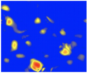
To visualize that $(M,PV_e)$ are slowly varying, figure 1 shows the short-time evolution of $M$ (a,c,e) and $PV_e$ (b,d,f). The system (2.43)–(2.48) evolves in a triply periodic domain from random, large-scale initial conditions with $\epsilon = O(0.1)$ (see § 3.1). To the eye, it is apparent that $(M,PV_e)$ are almost invariant for times $t = O(\epsilon ) \sim 10^{-1}$. We note that (2.43)–(2.48) have been non-dimensionalized using the advective time scale, such that one expects variation of the slow variable on the times $t = O(1)$.

Figure 1. Evolution of slow modes $M$ (a,c,e) and $PV_e$ (b,d,f) on short times of $t = O(\epsilon ) \sim 10^{-1}$, starting from large-scale random initial conditions at $t=0$. The two-dimensional (2-D) slices are taken with $x = {\rm \pi}$ held fixed. One can see that the slow modes $(M,PV_e)$ change very little over short times $t = O(\epsilon )$.

While $PV_e$ and $M$ represent the slow components, additional variables are needed to represent the fast components of the system, and thereby to completely specify the entire dynamics. Formally, we may divide the phase space into $(M, PV_e)$ and the wave complement $(W_1,W_2,u_m,v_m)$, where $(W_1,W_2)$ are analogous to dry inertia-gravity waves involving the vertical velocity $w$, and $({u}_m, {v}_m)$ are the horizontal mean velocities corresponding to inertial waves (Gill Reference Gill1982; Remmel & Smith Reference Remmel and Smith2009; Remmel Reference Remmel2010; Hernandez-Duenas et al. Reference Hernandez-Duenas, Smith and Stechmann2014).

Hence, we will make a change of variables to utilize the two quantities $PV_e$ and $M$ that characterize the slowly varying subspace.

The slow variables, $M$ and $PV_e$, will be the central focus of the remainder of the paper. They are analogous to the dry $PV$ that is the central focus of dry fast-wave averaging (e.g. Embid & Majda Reference Embid and Majda1996; Majda Reference Majda2003). In the dry case, in the limit of small $\epsilon$, the $PV$ variable has a remarkable property: it obeys a nonlinear evolution that is decoupled from the evolution of the fast waves. Here, in the moist case, our goal is to investigate the evolution of the slow variables $M$ and $PV_e$, and to see whether they have a decoupled evolution, or whether phase changes bring about coupling with waves.

2.3. Abstract form of the equations

Many systems related to dry atmospheric dynamics may be written in abstract form as

(2.59)\begin{equation} \frac{\partial \boldsymbol{v}}{\partial t}+ \mathscr{L}(\boldsymbol{v})+\mathscr{B}(\boldsymbol{v},\boldsymbol{v})=0, \end{equation}

where $\boldsymbol {v}$ is the state vector, the linear operator $\mathscr {L}$ includes the effects of rotation and buoyancy, and $\mathscr {B}$ is bilinear (Majda Reference Majda2003). On the other hand, the buoyancy changes its functional form across phase interfaces in dynamics with phase changes of water. In the latter case, (2.59) must be rewritten as

(2.60)\begin{equation} \frac{\partial \boldsymbol{v}}{\partial t} +H_u(\boldsymbol{v})\mathscr{L}_u(\boldsymbol{v}) +H_s(\boldsymbol{v})\mathscr{L}_s(\boldsymbol{v}) +\mathscr{B}(\boldsymbol{v},\boldsymbol{v})=0. \end{equation}

This is the abstract form of the model in (2.43)–(2.48), where the linear term $\mathscr {L}(\boldsymbol {v})$ has been replaced by $H_u(\boldsymbol {v})\mathscr {L}_u(\boldsymbol {v})+H_s(\boldsymbol {v})\mathscr {L}_s(\boldsymbol {v})$ to account for the effect of phase changes as described in (2.49)–(2.51a,b). Each of the linear operators, $\mathscr {L}_u$ and $\mathscr {L}_s$, is by itself a constant-coefficient operator. However, their prefactors, $H_u(\boldsymbol {v})$ and $H_s(\boldsymbol {v})$ depend on $\boldsymbol {v}$ such that $H_u(\boldsymbol {v})\mathscr {L}_u(\boldsymbol {v})+H_s(\boldsymbol {v})\mathscr {L}_s(\boldsymbol {v})$ is nonlinear.

Here, we assume existence of (2.43)–(2.48), and, consequently, the solution $\boldsymbol {v}^{\epsilon }(\boldsymbol {x},t)$ is assumed to be known for each value of $\epsilon$. Then for known $\boldsymbol {v}^{\epsilon }(\boldsymbol {x},t)$, the goal of fast-wave averaging is to assess the coupling between the slow and fast components of the flow. From this perspective, we treat the Heaviside functions $(H_u,H_s)$ as given functions of $(\boldsymbol {x},t)$ at the stages of the fast-wave-averaging analysis. Thus the abstract formulation is, a posteriori, restored to its original form (2.59) where $\mathscr {L}=H_u(\boldsymbol {x},t)\mathscr {L}_u+H_s(\boldsymbol {x},t)\mathscr {L}_s$. As a result, many of the techniques from prior fast-wave-averaging studies can be applied here to the case with phase changes.

2.4. Fast-wave averaging

Fast waves arise in (2.59) when the operator $\mathscr {L}$ has a large $O(\epsilon ^{-1})$ contribution for small $\epsilon \rightarrow 0$. In this case, the operator $\mathscr {L}$ may be decomposed as $\mathscr {L}=\epsilon ^{-1}\mathscr {L}_{*}+\mathscr {L}_0$, so that (2.59) may be rewritten as

(2.61)\begin{equation} \frac{\partial \boldsymbol{v}}{\partial t}+\epsilon^{{-}1} \mathscr{L}_{*}(\boldsymbol{v})+ \mathscr{L}_{0}(\boldsymbol{v}) + \mathscr{B}(\boldsymbol{v},\boldsymbol{v})=0, \quad \boldsymbol{v}(\boldsymbol{x},0) = \bar{v}(\boldsymbol{x}) \end{equation}

where the dominant terms are identified by the multiplier $\epsilon ^{-1}$ and $\bar {v}(\boldsymbol {x})$ is the initial state. As discussed, we treat phase boundaries $(H_u,H_s)$ as known functions of $(\boldsymbol {x},t)$ for the fast-wave averaging analysis, and proceed to analyse (2.61) together with

(2.62)\begin{equation} \mathscr{L}=H_u \mathscr{L}_u+H_s \mathscr{L}_s = \epsilon^{{-}1}\mathscr{L}_* + \mathscr{L}_0, \end{equation}

for given $(H_u,H_s)$.

The idea of fast-wave averaging is to use a two-time expansion

(2.63)\begin{equation} \boldsymbol{v}^{\epsilon}(\boldsymbol{x},t) = \boldsymbol{v}^{0}(\boldsymbol{x},t,\tau) + \epsilon \boldsymbol{v}^{1}(\boldsymbol{x},t,\tau) + \cdots, \quad \epsilon\rightarrow 0, \end{equation}

where $\tau = t/\epsilon$ is the fast time scale. Inserting (2.63) into (2.61), and collecting terms order-by-order in $\epsilon$, leads to a series of initial value problems whose solutions may be found explicitly in terms of the initial state $\bar {v}(\boldsymbol {x})$. The condition to suppress secular growth of $\boldsymbol {v}^{\; 1}$ is referred to as the fast-wave-averaged equation (Majda Reference Majda2003). Since phase interfaces are determined by the complete (thermo)dynamics, they have a fast component (dependence on $\tau$ in the two-time expansion). Therefore, a main new element of the formulation is the $\tau$ dependence in the linear operator $\mathscr {L}_*(t, \tau )$. In the limit $\epsilon \rightarrow 0$, $\tau =t/\epsilon \rightarrow \infty$ with $t = O(1)$, the fast-wave-averaged equation is thus given by

(2.64)$$\begin{gather} \dfrac{\partial \bar{v}(\boldsymbol{x},t)}{\partial t}=\lim_{\tau\rightarrow\infty}\dfrac{1}{\tau}\int_0^{\tau}\left\{ \left( \int_0^{s} \frac{\partial \mathscr{L}_*(t,s') }{\partial t}\,\textrm{d}s'\right) \bar{v} - \exp\left({ \int_0^{s} \mathscr{L}_*(t,s') \,\textrm{d}s'}\right)\right. \nonumber\\ \times \left[ \mathscr{L}_0(t,s)\left(\exp\left({- \int_0^{s} \mathscr{L}_*(t,s') \,\textrm{d}s'}\right)\bar{v}\right)\right.\nonumber\\ \left.\left.+\mathscr{B}\left(\exp\left({- \int_0^{s} \mathscr{L}_*(t,s') \,\textrm{d}s'}\right)\bar{v},\exp\left({- \int_0^{s} \mathscr{L}_*(t,s') \,\textrm{d}s'}\right)\bar{v}\right)\right] \right\}\,\textrm{d}s. \end{gather}$$

Another significant difference from the dry analysis is that the calculations to assess coupling on the right-hand side of (2.64) must be performed in physical space, rather than relying on Fourier analysis, owing to the piecewise nature of the buoyancy operator.

For compactness, most of the details to derive (2.64), and its projection onto $(M,PV_e)$ (see (2.72) and (2.73)), are presented elsewhere (Zhang et al. Reference Zhang, Smith and Stechmann2021). A sketch of the steps to arrive at (2.64) is given in Appendix A. In addition, the terms appearing in the final result (2.72)–(2.73) can be understood by comparison with the structure of $(M,PV_e)$ equations (2.53) and (2.56), as will be further explained at the end of the next section, § 2.5.

2.5. Fast-wave-averaged equations for $M$ and $PV_e$

To focus on the evolution of the slow variables $M$ and $PV_e$, and possible decoupling of their evolution from fast oscillations, we may project (2.64) onto the first two components of $\bar {v} = (M,PV_e,W_1,W_2,u_m,v_m)|_{\tau =0}$. To this end, let us separate slow and fast components using the following definitions:

(2.65)\begin{equation} \bar{v}(\boldsymbol{x},t) = \bar{v}_{(M,PV_e)}(\boldsymbol{x},t) + \bar{v}_{(W)}(\boldsymbol{x},t), \end{equation}

where

(2.66a,b)$$\begin{gather} \bar{v}_{(M,PV_e)}(\boldsymbol{x}, t) = \left( \begin{matrix} M(\boldsymbol{x},t)\\ PV_e(\boldsymbol{x},t)\\ 0\\ 0\\ 0\\ 0 \end{matrix} \right),\quad \bar{v}_{(W)}(\boldsymbol{x}, t) = \left( \begin{matrix} 0\\ 0\\ W_1(\boldsymbol{x},t,0)\\ W_2(\boldsymbol{x},t,0)\\ u_m(\boldsymbol{x},t,0)\\ v_m(\boldsymbol{x},t,0) \end{matrix} \right)\!. \end{gather}$$

The nomenclature ‘slow’ and ‘fast’ follows naturally from $\mathscr {L}_*\bar {v}_{(M,PV_e)} = 0$ while $\mathscr {L}_* \bar {v}_{(W)} \neq 0$. For ease of notation in the following evolution equations, we introduce the quantity

(2.67)\begin{equation} \bar{v}_{(W')}= \exp\left({ \int_0^{s} \mathscr{L}_*(t,s') \,\textrm{d}s'}\right) \bar{v}_{(W)}. \end{equation}

The fast-wave-averaged equation for the slow variable $M$ may be written as

(2.68)$$\begin{gather} \frac{\partial M(\boldsymbol{x},t)}{\partial t} ={-}\lim_{\tau \rightarrow \infty} \left( \frac{1}{\tau} \int_0^{\tau} \boldsymbol{u}_{(M,PV_e)}(\boldsymbol{x},t,s)\,\textrm{d}s +\frac{1}{\tau} \int_0^{\tau} \boldsymbol{u}_{(W')}(\boldsymbol{x},t,s)\,\textrm{d}s \right) \boldsymbol{\cdot} \boldsymbol{\nabla} M(\boldsymbol{x},t), \end{gather}$$

where $\boldsymbol {\nabla } M$ does not depend on $\tau$, and thus may be taken outside of the integrals. The velocity $\boldsymbol {u}_{(M,PV_e)}$ associated with $(M,PV_e)$ is found from $(M,PV_e)$ inversion,

(2.69)\begin{equation} \nabla_h^2 \psi + \frac{\partial }{\partial z} \left[H_u\left(\frac{1}{2} \frac{\partial \psi}{\partial z} + \frac{1}{2} M\right)\right] + \frac{\partial }{\partial z} \left[H_s\left(\frac{\partial \psi}{\partial z} + q_{vs}\right)\right] = PV_e, \end{equation}

where

(2.70a,b)\begin{align} \boldsymbol{u}_{(M,PV_e)} = \left(-\frac{\partial \psi}{\partial y},\frac{\partial \psi}{\partial x},0 \right),\quad {\theta_e}_{(M,PV_e)} = \frac{1}{2}H_u\left(\frac{\partial \psi}{\partial z}+ M \right) + H_s\left(\frac{\partial \psi}{\partial z} + q_{vs} \right). \end{align}

Relation (2.69) is one of the formulae to prescribe the transformation between $(u,v,w,\theta _e,q_t)$ and $(M,PV_e,W_1,W_2,u_m,v_m)$, with the wave complement set equal to zero, and is the analogue of $PV$ inversion in the dry dynamics (Smith & Stechmann Reference Smith and Stechmann2017; Wetzel et al. Reference Wetzel, Smith, Stechmann and Martin2019b, Reference Wetzel, Smith, Stechmann, Martin and Zhang2020). Once $\boldsymbol {u}_{(M,PV_e)}$ has been found from $(M,PV_e)$ inversion, one may compute $\boldsymbol {u}_{(W)} = \boldsymbol {u} - \boldsymbol {u}_{(M,PV_e)}$, and then use (2.67) to compute $\boldsymbol {u}_{(W')} \sim \boldsymbol {u}_{(W)}, \epsilon \rightarrow 0$.

To aid in the interpretation of (2.68), we use the notation $\langle f \rangle$ to define the time average of any function $f(\boldsymbol {x},t,\tau )$, as follows:

(2.71)\begin{equation} \langle f \rangle (\boldsymbol{x}, t) = \lim_{\tau \rightarrow \infty} \frac{1}{\tau} \int_0^{\tau} f(\boldsymbol{x},t,s)\,\textrm{d}s. \end{equation}

Using the bracket $\langle \ \rangle$ notation, the $M$-evolution equation (2.68) becomes

(2.72)\begin{equation} \frac{\partial M(\boldsymbol{x},t)}{\partial t} ={-}\langle \boldsymbol{u}_{(M,PV_e)} \rangle (\boldsymbol{x},t) \boldsymbol{\cdot} \boldsymbol{\nabla} M(\boldsymbol{x},t) - \langle \boldsymbol{u}_{(W')} \rangle (\boldsymbol{x},t) \boldsymbol{\cdot} \boldsymbol{\nabla} M(\boldsymbol{x},t), \end{equation}

in which there are two different contributions involving time-averaged velocity fields, $\langle \boldsymbol {u}_{(M,PV_e)} \rangle$ and $\langle \boldsymbol {u}_{(W')} \rangle$.

One of the significant differences between the dry case and phase-change case can now be seen. In particular, in the dry case, a dichotomy exists: the vortical eigenmode is slow, and the wave eigenmode is fast. In the phase-change case, this clean dichotomy no longer exists. As one indication of this, notice that the Heaviside functions $H_u$ and $H_s$ in (2.69) are influenced by waves. Therefore, the PDE in (2.69) has parameters ($H_u$ and $H_s$) that include fast-wave oscillations, and the solution $\psi$ will also be influenced by fast wave oscillations. Similarly, since the velocity $\boldsymbol {u}_{(M,PV_e)}$ is calculated from $\psi$ via (2.70a,b), it too is influenced by fast-wave oscillations. Interestingly, though, the quantities $PV_e$ and $M$ are indeed purely slow quantities, as indicated above, even though other quantities ($\psi ,\boldsymbol {u}_{(M,PV_e)}$, etc.) that are derived from $PV_e$ and $M$ are not purely slow quantities. Hence, in the phase-change case, one must analyse the average $\langle \boldsymbol {u}_{(M,PV_e)} \rangle$ as $\tau \rightarrow \infty$ in order to know the evolution of the slow variable $M$ in (2.72). On the other hand, in the dry case (or purely saturated case without phase changes), one has $\langle \boldsymbol {u}_{(M,PV_e)} \rangle = \boldsymbol {u}_{(M,PV_e)}$.

Using inversion formulae, and similar to the decomposition $\boldsymbol {u} = \boldsymbol {u}_{(M,PV_e)} + \boldsymbol {u}_{(W)}$, all primary variables $(u,v,w,\theta _e,q_t)$ may be decomposed into a component associated with $(M,PV_e)$ and a component associated with the waves $(W)$. Although there is $\tau$ dependence remaining in the $(M,PV_e)$ part, for the sake of simplicity and continuity with previous literature, we proceed to adopt the language convention that slow refers to $(\boldsymbol {\cdot })_{(M,PV_e)}$, while fast refers to $(\boldsymbol {\cdot })_{(W)}$. Using that convention, slow–slow (fast–fast) nonlinear interactions involve products between two quantities associated with $(M,PV_e)$ ($W$). Mixed slow–fast and fast–slowquadratic terms involve one of each type. Thus the first (second) term on the right-hand side of (2.72) is a slow–slow (fast–slow) term.

Figure 2 shows the short time evolution of the total water $q_t$ (panels (a,d,g)), along with the slow part $q_{t(M,PV_e)}$ and the fast part $q_{t(W)}$. The simulation is the same as in figure 1 (decay from large-scale initial conditions with $\epsilon = O(0.1)$), and short times correspond to $t = O(\epsilon ) \sim 10^{-1}$. Despite the $\tau$ dependence of $q_{t(M,PV_e)}$, it changes very little at large scales, while the variation of the unbalanced water $q_{t(W)}$ is much more significant. Our goal is to assess how the slow flow components are influenced by the fast components on $O(1)$ time scales, and in particular we use fast-wave averaging to study how the slow modes $(M,PV_e)$ are coupled to waves by analysing the nonlinear terms on the right-hand side of the $M$-equation (2.72).

Figure 2. Short-time evolution of total water $q_t = q_{t(M, PV_e)} + q_{t(W)}$ (a,d,g), slow water $q_{t(M, PV_e)}$ (b,e,h) and fast water $q_{t(W)}$ (c,f,i). The simulation is the same as in figure 1, and 2-D slices have $x = {\rm \pi}$ held fixed. The saturation threshold $q_{vs} = 0.5$, such that red corresponds to liquid water and blue corresponds to water vapour. The slow component $q_{t(M,PV_e)}$ changes very little on times $t = O(\epsilon )$, while the fast component $q_{t(W)}$ shows wave-like behaviour with $O(1)$ amplitude variation at fixed ${\boldsymbol {x}}$ over times $t = O(\epsilon )$.

To complete the picture, the fast-wave-averaged equation for $PV_e$ has also been derived from (2.64), and may be written as

(2.73)\begin{align} -\frac{\partial PV_e(\boldsymbol{x},t)}{\partial t} &= \langle \boldsymbol{u}_{(M,PV_e)} \rangle (\boldsymbol{x},t) \boldsymbol{\cdot} \boldsymbol{\nabla} PV_e(\boldsymbol{x},t) + \langle \boldsymbol{u}_{(W')} \rangle (\boldsymbol{x},t) \boldsymbol{\cdot} \boldsymbol{\nabla} PV_e(\boldsymbol{x},t) \nonumber\\ &\quad + \langle\frac{\partial \boldsymbol{u}_{(M,PV_e)}}{\partial z} \boldsymbol{\cdot} \boldsymbol{\nabla} {\theta_e}_{(M,PV_e)} \rangle (\boldsymbol{x},t) + \langle\frac{\partial \boldsymbol{u}_{(W')}}{\partial z} \boldsymbol{\cdot} \boldsymbol{\nabla} {\theta_e}_{(M,PV_e)} \rangle (\boldsymbol{x},t) \nonumber\\ &\quad+ \langle\frac{\partial \boldsymbol{u}_{(M,PV_e)}}{\partial z} \boldsymbol{\cdot} \boldsymbol{\nabla} {\theta_e}_{(W')} \rangle (\boldsymbol{x},t) + \langle\frac{\partial \boldsymbol{u}_{(W')}}{\partial z} \boldsymbol{\cdot} \boldsymbol{\nabla} {\theta_e}_{(W')} \rangle (\boldsymbol{x},t) \nonumber\\ &\quad+\langle \xi_{(M,PV_e)} (-{w_z}_{(W')})\rangle(\boldsymbol{x},t) + \langle \xi_{(W')} (-{w_z}_{(W')})\rangle(\boldsymbol{x},t) \nonumber\\ &\quad+\langle {w_x}_{(W')} {v_z}_{(M,PV_e)} -{w_y}_{(W')} {u_z}_{(M,PV_e)} \rangle(\boldsymbol{x},t) \nonumber\\ &\quad+\langle {w_x}_{(W')} {v_z}_{(W')} -{w_y}_{(W')} {u_z}_{(W')} \rangle(\boldsymbol{x},t). \end{align}

As mentioned above, the details to derive (2.72) and (2.73) are given in Zhang et al. (Reference Zhang, Smith and Stechmann2021). However, one can see the origin of the coupling terms by direct comparison with the original $(M,PV_e)$ evolution equations given by (2.53) and (2.56). Notice that the terms on the right-hand side of (2.72) and (2.73) are appropriate time averages of terms in (2.53) and (2.56), respectively, after the decomposition of all primary variables $(\boldsymbol {u},\theta _e,q_t)$ into their $(M,PV_e)$ and $(W)$ components. On the other hand, some terms are identically zero following the decomposition and averaging, which can be shown using the explicit structure of the operators in $\mathscr {L}_*, \mathscr {L}_0$ and $\mathscr {B}$ appearing in (2.64).

3.1. Numerical method

The three-dimensional (3-D) moist Boussinesq equations with two phases of water (vapour and liquid) are simulated in a $2{\rm \pi}$-periodic domain using a dealiased, pseudo-spectral code. Calculations with spatial resolutions $128 \times 128 \times 128$ and $256 \times 256 \times 256$ are compared to ensure that the results are insensitive to resolution, e.g. for the $O(1)$ time averages in (2.73) contributing to the evolution of the slow variable $PV_e$. The comparison provides confidence in the robustness of our results, especially for the smallest value of the Rossby and Froude numbers ($\epsilon \sim 10^{-3}$).

After transferring the physical space equations into Fourier space, a third-order Runge–Kutta time-stepping scheme solves the coupled system of ordinary differential equations (ODEs) resulting from discretization of the wavevector. Linear rotation and buoyancy terms are treated explicitly, and the nonlinear terms are calculated in physical space with implementation of FFTW (http://www.fftw.org/). A pressure solver enforces the incompressibility constraint, and viscous linear terms are included using an integrating factor. A hyperviscosity is used instead of the normal viscosity to induce dissipation only at the smallest scales. For example, in the momentum equation, the hyperviscosity takes the form

(3.1)\begin{equation} ({-}1)^{p+1} \nu(\nabla^2)^p \boldsymbol{v}, \end{equation}

where we use $p = 8$. The coefficient $\nu$ has the structure

(3.2)\begin{equation} \nu = 2.5 \left(\dfrac{E_{\nu}(k_m,t)}{k_m} \right)^{1/2}k_m^{2-2p}, \end{equation}

where $k_m$ is the highest available wavenumber and $E_{\nu }$ is the kinetic energy in the wavenumber shell associated with $k_m$. The spherical shell associated with wavenumber $k_i$ includes all wavenumbers satisfying $(i - 1) \Delta k < (\boldsymbol {k}\boldsymbol {\cdot }\boldsymbol {k})^{1/2} \leq i \Delta k, \Delta k = (2 {\rm \pi})/L$, and $L$ is length of the box (in our case $L = 2 {\rm \pi}$), where $i = 1, \ldots , N$ (in $128^3$ spatial resolutions case $N = 43$).

Similar expressions are used in the equations for equivalent potential temperature $\theta _e$ and water $q_t$ (Spyksma et al. Reference Spyksma, Bartello and Yau2006; Hernandez-Duenas et al. Reference Hernandez-Duenas, Majda, Smith and Stechmann2013).

3.3. Cloud fraction

During the simulations, the formulae $q_v = \min (q_t,q_{vs})$, $q_l = \max (0, q_t - q_{vs})$ are used to determine vapour $q_v$ and liquid water $q_l$ from total water $q_t$ and saturation threshold $q_{vs}$.

By adjusting the constant parameter $q_{vs}$, one may control the initial cloud fraction quantified by the cloud indicator $H_s(q_t - q_{vs})$. In § 4, the cloud fraction will be calculated as the $L^1$ norm of the cloud indicator $H_s(q_t - q_{vs})$. During the $O(1)$-time evolution, for a small amount of initial $\|H_s(q_t - q_{vs})\|_1$ with value less than $\leq 30\,\%$ of the domain, the fluctuation of $\|H_s(q_t - q_{vs})\|_1$ over time is quite small (1 %–2 %). Thus, for all practical purposes, the cloud fraction can be considered as fixed for the discussion in § 4.1. We note that large initial $\|H_s(q_t - q_{vs})\|_1$, with value $\geq 70\,\%$ of the domain, leads to significant fluctuations of $\|H_s(q_t - q_{vs})\|_1$ in time.

In §§ 4.1 and 5.1, the large-scale random initial conditions with $q_{vs} = 0.5$ lead to 22 % initial cloud fraction. For the moist bubble set-up discussed in § 4.2, we use the value $q_{vs} = 0.1$ corresponding to cloud fraction $28\,\%$. For one of the sensitivity studies, we vary $q_{vs}$ within the context of the large-scale random initial conditions, comparing results for the values $q_{vs} = 10, 1.5, 1, 0.5, 0, -0.5, -0.8, -1.5, -10$, such that we obtain cloud fractions increasing from $0\,\%$ to $100\,\%$, respectively.

3.4. Large-scale, random initial conditions

For most cases in § 4, we consider decay from large-scale, random initial conditions. The spectral density for all variables $(u,v,w,\theta _e,q_t)$ is a Gaussian function given by

(3.4)\begin{equation} F(k) = \epsilon_f \dfrac{\exp ({-}0.5(k- k_f)^2/s^2)}{(2 {\rm \pi})^{1/2} s} \end{equation}

where $s=1$ is standard deviation, $k_f=3$ is the peak wavenumber of the force and $\epsilon _f = O(1)$ is the energy input rate. Furthermore, the $k$ values are restricted to the interval $[1,5]$. Upon the change of variable from $(u,v,w,\theta _e,q_t)$ to $(M,PV_e,W_1,W_2,u_m,v_m)$, the slow $(M,PV_e)$ and fast $(W)$ components have comparable spectral density levels in wavenumbers $[1,5]$.

As a result, the initial conditions contain substantial contributions from waves, and, in this sense, the initial conditions are unbalanced.

For specific choices of the initial distinguished parameter $\epsilon$ (based on maximum magnitude of the initial velocity) and saturation threshold $q_{vs}$, the system evolves according to moist Boussinesq dynamics with phase changes of water. Figure 3 shows 2-D slices of the initial variables $u$ and $\psi$ constructed from aforementioned random initial condition.

Figure 3. Two-dimensional slices (at $x={\rm \pi}$) of the zonal velocity $u$ (a) and the stream function $\psi$ (b) at time $t=0$, visualizing the random large-scale initial conditions for these fields.

3.5. Evaluation of nonlinear terms in the fast-wave-averaged equation for $PV_e$

As discussed in § 2.5, the $(M, PV_e)$-evolution equations derived from fast-wave averaging have the explicit expressions (2.72) and (2.73). With a closer look at the $PV_e$ equation, the nonlinear terms appearing in the right-hand side of (2.73) contain slow–slow, fast–slow, slow–fast, fast–fast interactions.

We would like to analyse each of these nonlinear terms from (2.73), in the limit $\epsilon \to 0$.

To provide some context for the terms in (2.73), it is helpful to summarize what happens as $\epsilon \to 0$ in two related cases from earlier literature, and then to compare with the present situation. First, for the case of dry dynamics, only the slow–slow term $\boldsymbol {u}_{(PV)} \boldsymbol {\cdot } \boldsymbol {\nabla } PV$ is non-zero, which means the slowly varying evolution is decoupled from the fast waves (Embid & Majda Reference Embid and Majda1996, Reference Embid and Majda1998; Majda & Embid Reference Majda and Embid1998; Majda Reference Majda2003). Second, for the moist case but with balanced initial conditions (i.e. with initial conditions without waves), only slow–slow terms appear in the $(M,PV_e)$ limiting dynamics (Smith & Stechmann Reference Smith and Stechmann2017). However, returning now to the setting of the present paper with initial conditions that are unbalanced, one cannot, a priori, show that all of the fast–fast and fast–slow terms in (2.72) and (2.73) are zero.

Thus, phase changes lead to potential sources of feedback from fast oscillations onto the evolution of the slow modes $(M, PV_e)$. The feedback may originate directly from the fast components $(W)$, or indirectly at phase interfaces through $(M,PV_e)$ inversion, and is manifested through time averages over fast time scales.

Our purpose here is to assess the terms in (2.72) and (2.73) in numerical simulations.

Here we perform a numerical assessment for small values of $\epsilon$, and investigate trends for decreasing $\epsilon$.

For the $PV_e$-equation (2.73), the averages to be measured in the simulations at finite $\epsilon$ are the following. Slow–slow (terms 1, 3):

(3.5)\begin{gather} \frac{1}{T} \int_{0}^{T} \boldsymbol{u}_{(M,PV_e)}(\boldsymbol{x},t') \boldsymbol{\cdot} \boldsymbol{\nabla} PV_e(\boldsymbol{x},t')\,\textrm{d}t', \end{gather}

(3.6)\begin{gather} \frac{1}{T} \int_{0}^{T} \dfrac{\partial \boldsymbol{u}_{(M,PV_e)}(\boldsymbol{x},t')}{\partial z} \boldsymbol{\cdot}\boldsymbol{\nabla} \theta_{e(M,PV_e)}(\boldsymbol{x},t')\,\textrm{d}t'. \end{gather}

Fast–slow (terms 2, 4, 9):

(3.7)\begin{gather} \frac{1}{T} \int_{0}^{T} \boldsymbol{u}_{(W')}(\boldsymbol{x},t') \boldsymbol{\cdot} \boldsymbol{\nabla} PV_e(\boldsymbol{x},t')\,\textrm{d}t', \end{gather}

(3.8)\begin{gather} \frac{1}{T} \int_{0}^{T} \dfrac{\partial \boldsymbol{u}_{(W')}(\boldsymbol{x},t')}{\partial z} \boldsymbol{\cdot}\boldsymbol{\nabla} \theta_{e(M,PV_e)}(\boldsymbol{x},t')\,\textrm{d}t', \end{gather}

(3.9)\begin{gather} \frac{1}{T} \int_{0}^{T} [ {w_x}_{(W')}{v_z}_{(M,PV_e)} - {w_y}_{(W')}{u_z}_{(M,PV_e)}] (\boldsymbol{x},t') \,\textrm{d}t'. \end{gather}

Slow–fast (terms 5, 7):

(3.10)\begin{gather} \frac{1}{T} \int_{0}^{T} \dfrac{\partial \boldsymbol{u}_{(M,PV_e)}(\boldsymbol{x},t')}{\partial z} \boldsymbol{\cdot}\boldsymbol{\nabla} \theta_{e(W')}(\boldsymbol{x},t')\,\textrm{d}t', \end{gather}

(3.11)\begin{gather} \frac{1}{T} \int_{0}^{T} - \xi_{(M,PV_e)}{w_z}_{(W')} (\boldsymbol{x},t') \,\textrm{d}t'. \end{gather}

Fast–fast (terms 6, 8, 10):

(3.12) $$\begin{gather} \frac{1}{T} \int_{0}^{T} \left\{ \dfrac{\partial \boldsymbol{u}_{(W')}(\boldsymbol{x},t')}{\partial z} \boldsymbol{\cdot}\boldsymbol{\nabla} \theta_{e(W')}(\boldsymbol{x},t')\right.\nonumber\\ \left.+ \left[ -\xi_{(W')}{w_z}_{(W')} + {w_x}_{(W')}{v_z}_{(W')} - {w_y}_{(W')}{u_z}_{(W')}\right] (\boldsymbol{x},t') \vphantom{\dfrac{\partial \boldsymbol{u}_{(W')}(\boldsymbol{x},t')}{\partial z}}\right\}\,\textrm{d}t'. \end{gather}$$

The numerical quantities we monitor are discrete versions of (3.5)–(3.12) (and similar terms from the $M$-equation) with integration over total time $T$, which means that we average the data in the time window $t \in [0,T]$. Since the time-averaged quantities reach statistically steady state at $T \approx 0.3$, we present the case $T = 0.6$ as representative, unless otherwise stated. Note that long-time averages reflect loss of energy due to viscous decay in all variables, obscuring trends. Furthermore, a key diagnostic is the $L^2$ norm $\|\langle \cdot \rangle \|_2$ of an individual term or group of terms, which will always be normalized by its initial value for comparison between simulations with phase changes and purely saturated simulations without phase changes.

3.6. $(M,PV_e)$ inversion for finite $\epsilon$

After each time step of the numerical simulation, the updated state vector $(u,v,w,\theta _e,q_t)$ may be used in a post-processing step to find the updated fields $(M, PV_e, H_u, H_s)$. Then to compute the slow components $\boldsymbol {u}_{(M,PV_e)}$, $\theta _{e(M,PV_e)}$ and $q_{t(M,PV_e)}$, we use the finite-$\epsilon$ version of (2.69) given by

(3.13)$$\begin{gather} \nabla_h^2 \psi + \frac{\partial }{\partial z} \left[H_u\left(\frac{1}{2 - \epsilon} \frac{\partial \psi}{\partial z} + \frac{1 - \epsilon}{2 - \epsilon} M\right)\right]\nonumber\\ \quad + \frac{\partial }{\partial z} \left[H_s\left( \frac{1}{1 + \epsilon} \frac{\partial \psi}{\partial z} + \frac{\epsilon}{1 + \epsilon} M + (1-2\epsilon)q_{vs}\right)\right]\nonumber\\ = PV_e. \end{gather}$$

Following inversion of (3.13) to find the streamfuntion $\psi$, the relations (2.70a,b) are used to obtain $\boldsymbol {u}_{(M,PV_e)}$, $\theta _{e(M,PV_e)}$. Finally, the definition of $M$ given by (2.52), together with $\theta _{e(M,PV_e)}$, gives $q_{t(M,PV_e)}$.

For the numerical solution of (3.13), a centred-difference method was used, which, owing to the discontinuous coefficients introduced by phase boundaries $(H_u,H_s)$, is similar to the ghost fluid approach (Liu, Fedkiw & Kang Reference Liu, Fedkiw and Kang2000; Liu & Sideris Reference Liu and Sideris2003; Tzou & Stechmann Reference Tzou and Stechmann2019). The conjugate gradient method is then used to solve the discretized symmetric linear system and determine the stream function $\psi$. Here we adopt a simple version of the ghost-fluid method that does not use subcell information about the interface location, together with a Gaussian smoothing of the resulting $\psi$, such that gradient fields may be reliably computed in (3.5)–(3.12). A one-dimensional version of the Gaussian filter is given by

(3.14)\begin{equation} W[\psi](x) = \dfrac{1}{\sqrt{4{\rm \pi} s}} \int_{-\infty}^{\infty}\psi(x - y)\exp{\left(\dfrac{-y^2}{4s}\right)}\,{\textrm{d}y}, \end{equation}

where (3.14) is also known as a Weierstrass transformation. For the 3-D version we use the Gaussian–Weierstrass kernel $s=500$ in all three directions for resolution $256^3$ ($s=200$ in all directions for resolution $128^3$). A simplified test case shows quantitative agreement between this method and a subcell-location version of the ghost-fluid approach.

5.1. A closer look at simulated data

To explain the mechanism by which phase changes impact fast-wave averaging, we isolate points in the simulations where $O(1)$ time averages are larger than $O(\epsilon )$. We use the simulation with $\epsilon = O(10^{-2})$, random large-scale initial conditions and cloud fraction $22\,\%$. The goal is to explore the physical properties of these points where the time-average of fast–slow interactions is $O(10^{-1})$ instead of proportional to $\epsilon = O(10^{-2})$.

Specifically, we monitor the fast–slow term $\langle \boldsymbol {u}_{(W')} \rangle (\boldsymbol {x},t) \boldsymbol {\cdot } \boldsymbol {\nabla } M(\boldsymbol {x},t)$ in $M$-evolution equation (2.72), starting from random initial conditions. After time averaging, instead of taking the $L^2$ norm, we check all points ($x_0,y_0,z_0$) in the 3-D domain. A post-processing routine computes the absolute value $| ({1}/{T}) \int _{0}^{T} \boldsymbol {u}_{(W')}(\boldsymbol {x},t') \boldsymbol {\cdot } \boldsymbol {\nabla } M(\boldsymbol {x},t')\,\textrm {d}t' |$ for $T = 0.67$, and highlights every point whose time-averaged absolute value is greater than $O(0.1)$ (see figure 9c). Meanwhile, in order to observe the relationship between phase changes and such points, we also plot the initial cloud distribution (figure 9a), and the time-average $\langle H_s \rangle$ of the cloud indicator function $H_s$ (figure 9b). Note that $H_s$ is shorthand for $H_s(q_t-q_{vs})$. From the figure, one may observe the following: if the value $\langle H_s(x_0,y_0,z_0) \rangle$ is near 0 or 1, then this position ($x_0,y_0,z_0$) is away from a phase interface (blue colour in panel (b)); values $\langle H_s(x_0,y_0,z_0) \rangle \in [0.2, 0.8]$ indicate that this position experiences frequent change of phase (yellow colour in panel (b)).

Figure 9. Two-dimensional slices (at $x={\rm \pi}$) of the initial cloud indicator $H_s$ at $t = 0$ (a), time-averaged cloud indicator $\langle H_s \rangle$ (b) and absolute value $| \langle \boldsymbol {u}_{(W')} \boldsymbol {\cdot } \boldsymbol {\nabla } M \rangle |$ of a slow–fast term in the fast-time-averaged $M$-equation. Red areas in panel (a) represent clouds (liquid water where $q_t > q_{vs} = 0.5$). Yellow patterns in panel (b) indicate the regions where phase changes happen frequently; blue indicates that the region has remained vapour (value zero) or liquid (value unity) for the duration of the averaging window. Hot spots (yellow to red) in panel (c) indicate high values of the fast–slow coupling term.

A closer look at the hot spots (yellow–red colour) in figure 9(c) reveals interesting physical properties of the flow. For a specific point $(x_0,y_0,z_0) = (64,55,11)*(2{\rm \pi} /128) \approx (3.14, 2.70, 0.54)$, figure 10 demonstrates how the location alternates between unsaturated and saturated states (figure 10a). During the time $t \in [0,0.67]$, there are 23 time windows with $H_s(t,x_0,y_0,z_0) = 1$, and 22 time windows with $H_s(t,x_0,y_0,z_0) = 0$. Furthermore, figure 10(b) shows the time ratio that the wave spends in those two different states as a function of time window ($\text {time ratio} = \text {time in each window}/T$, where $T = 0.67$). One can see that more time is spent in the saturated state. Quantitatively, $58\,\%$ of the time is spent in the saturated state, compared with $42\,\%$ of the time in the unsaturated state. Close to a phase boundary, a wave spends more time in the saturated state because the frequencies have the relationship $(\sigma _u,\sigma _s) = (\sqrt {2}\epsilon ^{-1}, \epsilon ^{-1})$ (see (3.3a,b) and recall that $Fr_1 = Fr_2 = \epsilon$). Therefore, the non-zero frequency $\sigma _u$ in the unsaturated state is greater than $\sigma _s$ in the saturated state. Finally, figure 11 shows that $q_t$ has wave fluctuations crossing the saturation threshold, and it spends more time in the saturated state. Other physical variables exhibit similar behaviour.

Figure 10. (a) Plot of $H_s(t,\boldsymbol {x})$ versus time $t$ for $t \in [0, 0.67]$, with $H_s$ measured from a red-spot position $(x_0,y_0,z_0) \approx (3.14, 2.70, 0.54)$ in figure 9. There are 45 total alternating time windows: 23 for the saturated state and 22 for the unsaturated state. Quantitatively, $58\,\%$ of the time is spent in the saturated state, compared with $42\,\%$ time in the unsaturated state. (b) The green triangles represent the time ratio spent in unsaturated windows, while the red squares correspond to time spent in saturated windows ($\text {time ratio} = \text {time in each window}/T$, where $T = 0.67$).

Figure 11. Total water $q_t$ versus time $t$ at a fixed red point $(x_0,y_0,z_0) \approx (3.14, 2.70, 0.54)$ in figure 9. The green line is the saturation threshold $q_{vs}= 0.5$. The wave (purple curve) has different wavelengths/amplitudes in the saturated and unsaturated regions, located, respectively, above and below the threshold, leading to non-zero $O(1)$ time averages $\langle q_t(t,x_0,y_0,z_0)\rangle$.

Since more time is spent in the saturated phase (more time is spent in the wave crest than in the wave valley), $O(1)$ time averages are not zero.

To give a better feel for physical-space variability of the waves, figure 12 shows the wave part $u_{(W)}$ of the horizontal velocity $u = u_{(M, PV_e)} + u_{(W)}$, comparing waves in simulations with phase changes (panels (a,c,e,g), cloud fraction $22\,\%$) and without phase changes (panels (b,d,f,h), cloud fraction $100\,\%$). The set-up is decay from random initial conditions and the resolution is $128^3$. In panels (a,b) corresponding to time $t=0$, notice that the initial conditions of $u_{(W)}$ are slightly different, and this is because the inversion formula for extracting the waves involves Heaviside functions when phase changes are present, but has continuous coefficients when waves are absent. In panels (c,d) and (e,f), one can see that the variation of waves in both scenarios is significant for times $t = O(\epsilon )$. Moreover, smaller scale features are generated during the evolution with phase changes. Finally, panels (g,h) of figure 12 displays the absolute value of $\langle u_{(W)}\rangle$ for the two cases, using the averaging time $T=0.6$. Corroborating the findings in figure 11, there are locations with significantly higher time-averages $\langle u_{(W)}\rangle$ when phase boundaries are present (the white and red spots on the left).

Figure 12. Zonal waves $u_{(W)}$ in decay from random initial conditions during a simulation with phase changes (a,c,e,g, cloud fraction $22\,\%$) and a purely saturated simulation (b,d,f,h, cloud fraction $100\,\%$). From the first three rows at $t = 0, 0.02, 0.04$, one can see the development of smaller scales when phase changes are present. Panels (g,h) the absolute value of $\langle u_{(W)}\rangle$, using the averaging $T = 0.6$. There are locations with significantly higher time-averages $\langle u_{(W)}\rangle$ when phase boundaries are present (white and red spots on the left).

5.2. ODE system

In this section, we use a model system of ODEs to elucidate the nature of waves that oscillate between unsaturated and saturated regions of the flow. In particular, the ODE model has exact solutions corresponding to waves propagating across phase boundaries, with non-zero time averages, as has been observed in the moist Boussinesq system (figures 9 and 12).

The ODE model system arises from the 3-D Boussinesq moist dynamics when spatial variations are neglected (see Appendix B),

(5.1)\begin{gather} \frac{\textrm{d}w}{\textrm{d}t} = b = N_ub_u H_u + N_sb_s H_s, \end{gather}

(5.2)\begin{gather} \frac{\textrm{d}b_u}{\textrm{d}t} + N_u w = 0, \end{gather}

(5.3)\begin{gather} \frac{\textrm{d}b_s}{\textrm{d}t} + N_s w = 0. \end{gather}

Hence, the ODE system (5.1)–(5.3) describes time variation at a single point in space. Among the velocity components, only the $w$ equation is retained, leading to the simplest set-up that still retains waves. Phase boundaries in (5.1)–(5.3) are identified by the condition $b_u=b_s$, and the cloud indicator may be written as $H_s=H(b_s-b_u)$. In analogy with (3.3a,b) for the Boussinesq system, the waves represented by (5.1)–(5.3) have different frequencies associated with the different phases ($b_u,b_s$) and buoyancy parameters ($N_u,N_s$) (see Durran & Klemp (Reference Durran and Klemp1982a) and references therein). This is central for understanding figures 9 and 12.

For the asymptotic theory discussed in the next two sections, we consider the limiting dynamics for buoyancy frequencies $N_u, N_s \rightarrow \infty$, which is analogous to the limiting dynamics for $\epsilon ^{-1}\rightarrow \infty$ in the fast-wave-averaging analysis of the moist Boussinesq system (2.43)–(2.48). We continue to use the special parameter setting ${N_u}^{2} = 2{N_s}^2$ as in the numerical simulations, where $N_u, N_s$ are both positive.

5.2.1. General solution for ODE system in different phases

In order to solve (5.1)–(5.3) analytically, the key point is to define the invariant variable $M$.

For the ODE system, the definition of $M$ is $M = N_u^{-1}b_u - N_s^{-1}b_s$, which is defined as the linear combination of $b_u$ and $b_s$ that satisfies* $\textrm {d}M/\textrm {d}t = 0$. In the earlier PDE system in § 2.2, $M$ was defined in terms of different variables, $\theta _e$ and $q_t$, and in non-dimensional units, although the different $M$ definitions can be related via the relationship between the variables $(\theta _e,q_t)$ and the variables $(b_u,b_s)$ as shown in (2.16) or (2.51a,b). For both the ODE system and the PDE system, the motivation for the $M$ definition is the same: find the quantity that satisfies $\textrm {d}M/\textrm {d}t=0$ or $\textrm {D}M/\textrm {D}t=0$.

Since $\textrm {d}M/\textrm {d}t=0$, the value of $M$ is a parameter, and then $b_s = ({N_s^{}}/{N_u^{}})b_u - M N_s$. With the replacement of $b_s$ in the ODE system, we only need two variables at any given time to describe the evolution as

(5.4)\begin{gather} \dfrac{\textrm{d}w}{\textrm{d}t} = N_u b_u H_u + N_s\left(\dfrac{N_s^{}}{N_u^{}}b_u - M N_s\right) H_s , \end{gather}

(5.5)\begin{gather}\dfrac{\textrm{d}b_u}{\textrm{d}t} + N_u w = 0 . \end{gather}

The cloud indicator $H_s=H(b_s-b_u)$ follows from the condition $H_s=H(q_t-q_{vs})$, where $b_s \geq b_u$ corresponds to a saturated region while $b_s < b_u$ represents an unsaturated region (Marsico et al. Reference Marsico, Smith and Stechmann2019).

For an unsaturated region, $b_u > MN_sN_u/(N_s-N_u)$ yields

(5.6)\begin{equation} b_u'' + N_u^2b_u = 0, \end{equation}

followed by the general solution

(5.7)\begin{equation} b_u = c_{u1}\sin(N_ut) +c_{u2}\cos(N_ut). \end{equation}

For a saturated region, $b_u \leq MN_sN_u/(N_s-N_u)$ leads to

(5.8)\begin{equation} b_u'' + N_s^2b_u = MN_s^2N_u, \end{equation}

followed by the general solution

(5.9)\begin{equation} b_u = c_{s1}\sin(N_st) +c_{s2}\cos(N_st) + MN_u. \end{equation}

To find a nonlinear solution that switches phase, as a piecewise sine function, the main idea is to use variables $(w,b_u)$ in the unsaturated phase and then evolve the system forward in time until the saturation condition is reached. After that, we switch to using variables $(w,b_s)$ while in the saturated phase.

5.2.2. A simple solution example with $M = 0$

A simple solution of the nonlinear wave in the ODE system is now presented, for any ($b_u(t_0), w(t_0), M$), where $t_0$ is the initial time. The interesting case will be an alternating piecewise wave, which crosses the phase boundary repeatedly, passing back and forth between unsaturated and saturated regions. For simplicity, we demonstrate using an example with $M = 0$, which means that the phase boundary is exactly at $b_u=0$.

Without loss of generality, assume an initial buoyancy exactly at the phase boundary such that $b_u(t_0) = 0$, and set the initial vertical velocity $w(t_0) = a$, where $a$ is an arbitrary positive number. Note that $b'_u(t_0) = -N_uw(t_0) = -N_u a<0$, which indicates that the solution will enter the saturated region first. The analytical solution for this initial condition is given by

(5.10)\begin{equation} b_u(t) = \left\{ \begin{array}{ll} -\dfrac{aN_u}{N_s} \sin(N_s(t - t_0)) & t \in \left[t_0 + n {\mathcal{T}}, t_0 + \dfrac{\rm \pi}{N_s} + n{\mathcal{T}}\right],\\ a \sin\left(N_u\left(t - t_0 - \dfrac{\rm \pi}{N_s}\right)\right) & t \in \left[t_0 + \dfrac{\rm \pi}{N_s} + n{\mathcal{T}}, t_0 + (n+1){\mathcal{T}}\right], \end{array} \right. \end{equation}

where ${\mathcal {T}} = {{\rm \pi} }/{N_u} + {{\rm \pi} }/{N_s} \text { and } n = 0, 1, 2, \ldots$. Then, after one half-period at $t = t_0 + {\rm \pi}/ N_s$, the solution meets the phase interface at $b_u=0$ with $b_u(t_0 + {\rm \pi}/ N_s) = 0, b_u'(t_0 + {\rm \pi}/ N_s) = aN_u > 0$, which is the starting point for wave propagation in the unsaturated region.

Using (5.10), we can now calculate the time-averaged value $| ({1}/{T}) \int _0^{T} b_u(t) \,\textrm {d}t |$, to determine if there is a non-zero average when a phase boundary is present. Without loss of generality, we choose $a = 1$ and $N_u = \sqrt {2}N_s$. On the one hand, consider the purely unsaturated case without phase changes, in which case the analytical solution for $b_u(t)$ is a simple sine function with frequency $N_u$. In that case, for fixed averaging interval ${T}$, the average $| ({1}/{T}) \int _0^{T} b_u(t)\,\textrm {d}t | \leq {2}/{N_uT} \rightarrow 0$ as $N_u \rightarrow \infty$. On the other hand, if the phase interface is present, then we find the following relation:

(5.11)\begin{equation} \frac{2}{{\rm \pi} (1 + \sqrt{2})} - \frac{2}{N_u T} \leq | \frac{1}{T} \int_0^T b_u(t) \,\textrm{d}t | \leq \frac{2}{{\rm \pi} (1 + \sqrt{2})} + \frac{2}{N_u T},\quad N_u \rightarrow \infty, \end{equation}

which is strictly bounded away from zero. Figure 13 displays the solution (5.10), and clearly illustrates how different frequencies $N_u \neq N_s$ lead to non-zero time average of $b_u(t)$ as in (5.11). Most importantly, the same essential mechanism is observed in the 3-D Boussinesq simulations, as seen in figure 11.

Figure 13. Sketch of the piecewise solution to (5.10) for $M=0$ such that the phase interface is at $b_u=0$.