


1. Introduction
Hypersonic flow over a double cone represents a canonical case of shock-wave–boundary- layer interaction (Babinsky & Harvey Reference Babinsky and Harvey2011). A double cone can sustain a strong interaction phenomenon and obviate the finite-span effects of its two-dimensional counterpart (i.e. a double wedge). Therefore, hypersonic double-cone flows have been extensively studied to understand shock-induced separation and validate computational fluid dynamics (CFD) tools.
A series of 25°–55° double-cone experiments has been conducted at Calspan–University of Buffalo Research Center over the past two decades with a wide range of free-stream Mach numbers, Reynolds numbers and total enthalpies in the LENS I reflected shock tunnel and LENS XX expansion tunnel (Holden & Wadhams Reference Holden and Wadhams2003; Holden et al. Reference Holden, Wadhams, Candler and Harvey2003; Holden et al. Reference Holden, Wadhams, Maclean and Dufrene2015). Surface pressure and heat flux distributions were measured. Various numerical simulations have been performed and compared with the experiments (Gaitonde, Canupp & Holden Reference Gaitonde, Canupp and Holden2002; Nompelis, Candler & Holden Reference Nompelis, Candler and Holden2003; Druguet, Candler & Nompelis Reference Druguet, Candler and Nompelis2005; Knight et al. Reference Knight, Longo, Drikakis, Gaitonde, Lani, Nompelis, Reimann and Walpot2012; Hao & Wen Reference Hao and Wen2018a,Reference Hao and Wenb). However, these CFD validation campaigns were only a partial success. Under high-enthalpy conditions with evident vibrational excitation and chemical reactions, the CFD significantly underestimated the size of the separation region. In contrast, good agreement was usually obtained at low enthalpies. However, the axisymmetric simulations predicted a dramatically unsteady flow in some circumstances, whereas the experiments suggested the opposite (Knight et al. Reference Knight, Longo, Drikakis, Gaitonde, Lani, Nompelis, Reimann and Walpot2012). Currently, these discrepancies are still not understood.
Historically, flow unsteadiness in shock-wave–laminar boundary-layer interactions has received much less attention than turbulent ones. In hypersonic laminar flow over a double cone, unsteadiness may occur due to different physical mechanisms. Hornung, Gollan & Jacobs (Reference Hornung, Gollan and Jacobs2021) numerically studied axisymmetric double-cone flows with varying flow parameters. Pulsating unsteadiness was found to be an inviscid phenomenon consistent with the pulsation mode in supersonic spiked-body flows. In particular, the parameter space of the first and second cone angles was explored to determine the unsteadiness boundary. The lower boundary decreased to approach the shock detachment angle of the second cone as the first cone angle was decreased. Tumuklu, Theofilis & Levin (Reference Tumuklu, Theofilis and Levin2018) performed time-accurate direct Monte Carlo simulations of Mach 16 flows over the 25°–55° double cone with different unit Reynolds numbers. For the highest-Reynolds-number case, the Kelvin–Helmholtz instability arising in the shear layer and a bow-shock oscillation were captured with dominant frequencies of 45–70 and 2 kHz, respectively. Interestingly, the residuals algorithm identified a temporally stable axisymmetric global mode, highlighting a strong coupling between the separation region and shock system. Compared with the well-known pulsation mode and Kelvin–Helmholtz instability of an inviscid nature, the onset of global instability intrinsic to double-cone flows merits further investigation.
Nominally two-dimensional/axisymmetric laminar separation bubbles can sustain three-dimensional instabilities (Theofilis, Hein & Dallmann Reference Theofilis, Hein and Dallmann2000; Theofilis Reference Theofilis2011) with no upstream disturbances, which have been studied by the global stability analysis (GSA) approach. In the supersonic flow regime, global instabilities are further complicated by compressibility and complex shock structures. Robinet (Reference Robinet2007) observed low-frequency unsteady characteristics of shock impingement on a Mach 2.15 laminar boundary layer using direct numerical simulations (DNS), which stemmed from a supercritical Hopf bifurcation of the separated flow. Global stability analysis confirmed that the flow became globally unstable beyond a critical angle of the incident shock. Similarly, Hildebrand et al. (Reference Hildebrand, Dwivedi, Nichols, Jovanović and Candler2018) studied shock impingement on a Mach 5.92 laminar boundary layer. They found a stationary global mode at a supercritical shock angle, which can lead to the formation of streamwise streaks downstream of reattachment.
For a Mach 5 double-wedge flow, Sidharth et al. (Reference Sidharth, Dwivedi, Candler, & Nichols and W2018) found a stationary unstable mode beyond a critical deflection angle, which was attributed to the streamwise deceleration of the separated flow. At a supercritical deflection angle, multiple stationary and oscillating unstable modes were captured. Cao et al. (Reference Cao, Hao, Klioutchnikov, Olivier and Wen2021) observed streamwise streaks in heat flux on the ramp surface in hypersonic flow over a 15° compression corner with low-frequency unsteadiness using DNS. The two-dimensional base flow was found to be globally unstable by GSA, which identified one stationary and two oscillating modes. Good agreement was obtained between DNS and GSA in terms of the spanwise wavelengths of the streaks and dominant frequencies. More recently, the global stability of a Mach 7.7 compression corner flow was parametrically studied by Hao et al. (Reference Hao, Cao, Wen and Olivier2021) with different ramp angles and wall temperatures, which was closely linked with the emergence of secondary separation beneath the primary bubble. As the ramp angle was increased beyond a certain value, a long-wavelength stationary unstable mode first occurred, followed by a short-wavelength stationary mode and additional oscillating modes. Furthermore, it was found that the stability boundary can be well correlated in terms of a scaled ramp angle according to the triple-deck theory (Neiland Reference Neiland1969; Stewartson & Williams Reference Stewartson and Williams1969).
In previous GSA studies, only two-dimensional flow problems were considered, except that of Tumuklu et al. (Reference Tumuklu, Theofilis and Levin2018). However, their residuals analysis was restricted to axisymmetric scenarios with only temporally stable modes. The bifurcation of axisymmetric double-cone flows into three-dimensionality remains to be understood. To this end, hypersonic flow over the 25°–55° double-cone configuration is investigated numerically and theoretically in this study. Axisymmetric CFD and GSA are performed over a range of unit Reynolds numbers. The base flows are compared with existing experimental data and interpreted using the triple-deck theory. The corresponding linear stability spectra are then explored by assuming periodic perturbations in the azimuthal direction. Finally, DNS are performed to verify the GSA results and reveal the evolution of three-dimensional flow structures.
2. Geometric configuration and flow conditions
The experimental model tested in the LENS I and LENS XX tunnels is considered here, as shown in figure 1. The 25°–55° double cone has a sharp nose with two equal-length conical sections (L = 0.1016 m). A cylindrical coordinate system is constructed with the origin at the nose, the x direction along the cone axis, the r direction perpendicular to the axis and the ϕ direction satisfying the right-hand rule.

Figure 1. Schematic of the double-cone configuration.
The baseline flow conditions are taken from run 35 (Holden et al. Reference Holden, Wadhams, Candler and Harvey2003) with free-stream conditions M ∞ = 11.5, ρ ∞ = 5.515 × 10⁻⁴ kg m−3, T ∞ = 138.9 K, u ∞ = 2713 m s−1 and Re ∞ = 1.6 × 10⁵ m−1. Due to the low total enthalpy, the air is assumed to be calorically perfect with a constant specific heat ratio of 1.4. In fact, a certain amount of vibrational energy was frozen in the nozzle exit of the LENS I reflected shock tunnel. However, as shown by Nompelis et al. (Reference Nompelis, Candler and Holden2003), the inclusion of the vibrational energy and its weak accommodation at the wall only improved the predictive accuracy of the heat flux on the first cone. Therefore, no vibrational energy is considered in this study. The flow-field variables are non-dimensionalized using the free-stream parameters. The length of the conical section L is used as the characteristic length of the flow.
Three additional flow conditions are considered, with the free-stream density ρ ∞ decreased from the baseline value by a factor of 0.75, 0.5 and 0.33, while the other free-stream quantities remain unchanged. For convenience, these cases are labelled 0.75Re, 0.5Re and 0.33Re.
According to Hornung et al. (Reference Hornung, Gollan and Jacobs2021), the pulsation mode is enclosed in the lower and upper boundaries of the second cone angle (θ 2) for a given first cone angle (θ 1). The lower boundary is located above the shock detachment angle (θd) of the second cone with respect to M ∞. For the current flow conditions, θd is approximately 57° as determined from the Taylor‒Maccoll equations, which indicates that the considered 25°–55° double-cone flows sustain no inviscid unsteadiness.
3. Computational details
3.1. Governing equations
The governing equations are the compressible Navier–Stokes equations for a calorically perfect gas written in the following conservation form:
 \begin{equation}\frac{{\partial {\boldsymbol U}}}{{\partial t}} + \frac{{\partial {\boldsymbol F}}}{{\partial x}} + \frac{1}{r}\frac{{\partial (r{\boldsymbol G})}}{{\partial r}} + \frac{1}{r}\frac{{\partial {\boldsymbol H}}}{{\partial \phi }} = \frac{1}{r}{\boldsymbol Q},\end{equation}
where U = [ρ, ρu, ρv, ρw, ρE]T is the vector of conservative variables and the vectors of fluxes and source terms are given by
 \begin{gather}{\boldsymbol F} = \begin{bmatrix} {\rho u}\\ {\rho {u^2} + p}\\ {\rho vu}\\ {\rho wu}\\ {(\rho E + p)u} \end{bmatrix} + \begin{bmatrix} 0\\ {{\tau_{xx}}}\\ {{\tau_{rx}}}\\ {{\tau_{\phi x}}}\\ {u{\tau_{xx}} + v{\tau_{rx}} + w{\tau_{\phi x}} + {q_x}} \end{bmatrix},\end{gather}
 \begin{gather}{\boldsymbol G} = \begin{bmatrix} {\rho v}\\ {\rho uv}\\ {\rho {v^2} + p}\\ {\rho wv}\\ {(\rho E + p)v} \end{bmatrix} + \begin{bmatrix} 0\\ {{\tau_{xr}}}\\ {{\tau_{rr}}}\\ {{\tau_{\phi r}}}\\ {u{\tau_{xr}} + v{\tau_{rr}} + w{\tau_{\phi r}} + {q_r}} \end{bmatrix},\end{gather}
 \begin{gather}{\boldsymbol H} = \begin{bmatrix} {\rho w}\\ {\rho uw}\\ {\rho vw}\\ {\rho {w^2} + p}\\ {(\rho E + p)w} \end{bmatrix} + \begin{bmatrix} 0\\ {{\tau_{x\phi }}}\\ {{\tau_{r\phi }}}\\ {{\tau_{\phi \phi }}}\\ {u{\tau_{x\phi }} + v{\tau_{r\phi }} + w{\tau_{\phi \phi }} + {q_\phi }} \end{bmatrix},\end{gather}
 \begin{gather}{\boldsymbol Q} = \begin{bmatrix} 0\\ 0\\ {p + \rho {w^2} + {\tau_{\phi \phi }}}\\ { - \rho vw - {\tau_{r\phi }}}\\ 0 \end{bmatrix}.\end{gather}
In these expressions, ρ is the density, u, v and w are the flow velocities in the x, r and ϕ directions, respectively, p is the pressure and E is the total energy per unit mass. The shear stresses are calculated according to a Newtonian fluid and the Stokes hypothesis as
 \begin{gather}{\tau _{xx}} ={-} \mu \left[ {2\frac{{\partial u}}{{\partial x}} - \frac{2}{3}\left( {\frac{{\partial u}}{{\partial x}} + \frac{{\partial v}}{{\partial r}} + \frac{1}{r}\frac{{\partial w}}{{\partial \phi }} + \frac{v}{r}} \right)} \right],\end{gather}
 \begin{gather}{\tau _{rr}} ={-} \mu \left[ {2\frac{{\partial v}}{{\partial r}} - \frac{2}{3}\left( {\frac{{\partial u}}{{\partial x}} + \frac{{\partial v}}{{\partial r}} + \frac{1}{r}\frac{{\partial w}}{{\partial \phi }} + \frac{v}{r}} \right)} \right],\end{gather}
 \begin{gather}{\tau _{\phi \phi }} ={-} \mu \left[ {2\left( {\frac{1}{r}\frac{{\partial w}}{{\partial \phi }} + \frac{v}{r}} \right) - \frac{2}{3}\left( {\frac{{\partial u}}{{\partial x}} + \frac{{\partial v}}{{\partial r}} + \frac{1}{r}\frac{{\partial w}}{{\partial \phi }} + \frac{v}{r}} \right)} \right],\end{gather}
 \begin{gather}{\tau _{xr}} = {\tau _{rx}} ={-} \mu \left( {\frac{{\partial u}}{{\partial r}} + \frac{{\partial v}}{{\partial x}}} \right),\end{gather}
 \begin{gather}{\tau _{x\phi }} = {\tau _{\phi x}} ={-} \mu \left( {\frac{1}{r}\frac{{\partial u}}{{\partial \phi }} + \frac{{\partial w}}{{\partial x}}} \right),\end{gather}
 \begin{gather}{\tau _{r\phi }} = {\tau _{\phi r}} ={-} \mu \left( {\frac{1}{r}\frac{{\partial v}}{{\partial \phi }} + \frac{{\partial w}}{{\partial r}} - \frac{w}{r}} \right),\end{gather}
where μ is the dynamic viscosity evaluated using Sutherland's law. The vector of heat conduction is modelled according to Fourier's law as
 \begin{equation}{q_x} ={-} k\frac{{\partial T}}{{\partial x}},\quad {q_r} ={-} k\frac{{\partial T}}{{\partial r}},\quad {q_\phi } ={-} k\frac{1}{r}\frac{{\partial T}}{{\partial \phi }},\end{equation}
where k is the coefficient of thermal conductivity evaluated using a constant Prandtl number of 0.72.
It is assumed that U can be decomposed into an axisymmetric steady solution and a three-dimensional small-amplitude perturbation as
 \begin{equation}{\boldsymbol U}(x,r,\phi ,t) = \bar{{\boldsymbol U}}(x,r) + {\boldsymbol U^{\prime}}(x,r,\phi ,t).\end{equation}
Hereafter, the overbar and prime denote base-flow and perturbation variables, respectively.
3.2. Base-flow solver
The governing equations of the base flow can be readily obtained from (3.1) by assuming
 \begin{equation}\bar{w} = 0,\quad \overline {\frac{\partial }{{\partial \phi }}} = 0.\end{equation}
The integral form of the axisymmetric governing equations can then be obtained by applying the divergence theorem to a finite-volume cell of unit radian in the azimuthal direction as
 \begin{equation}\oint_S {(\bar{{\boldsymbol F}}{n_x} + \bar{{\boldsymbol G}}{n_r})\,\textrm{d}S} = \int_V {\frac{1}{r}\bar{{\boldsymbol Q}}\,\textrm{d}V} ,\end{equation}
where nx and nr are the components of the unit normal vector of the control surface, S is the area of the cell surface and V is the cell volume. The discrete form of (3.15) can be expressed as
 \begin{equation}\frac{1}{V}\sum\limits_f {{{(\bar{{\boldsymbol F}}{n_x} + \bar{{\boldsymbol G}}{n_r})}_f}{S_f}} = \frac{1}{{{r_c}}}{\bar{{\boldsymbol Q}}_c},\end{equation}
where the subscripts f and c denote face- and cell-averaged values, respectively.
The base-flow solutions are obtained using an in-house multiblock parallel finite-volume solver called PHAROS (Hao, Wang & Lee Reference Hao, Wang and Lee2016; Hao & Wen Reference Hao and Wen2020). The modified Steger–Warming scheme (MacCormack Reference Maccormack2014) is used to calculate the inviscid fluxes, which is extended to a second order by the monotone upstream-centred schemes for conservation law reconstruction (van Leer Reference Van Leer1979). The viscous fluxes are computed using the second-order central difference. An implicit line relaxation method (Wright, Candler & Bose Reference Wright, Candler and Bose1998) is used for pseudo time stepping.
The boundary conditions are given as follows. Free-stream conditions are applied to the far-field boundary, whereas the outflow boundary conditions are determined using a simple extrapolation. The model surface is assumed to have no slip with a fixed wall temperature Tw = 300 K corresponding to a wall temperature ratio Tw/T 0 = 0.079, where T 0 is the free-stream total temperature.
Numerical simulations are run with a constant Courant–Friedrichs–Lewy number of 103 until iterative convergence. For all cases, the Euclidean norm of the density residual is reduced by at least ten orders of magnitude, and the distributions of surface quantities no longer change in successive iterations. No self-sustained instabilities are supported by the considered axisymmetric double-cone flows.
3.3. Global stability analysis
The governing equations of U' can be obtained by substituting (3.13) into the governing equations (3.1) and neglecting higher-order terms as
 \begin{equation}\frac{{\partial {\boldsymbol U^{\prime}}}}{{\partial t}} + \frac{{\partial {\boldsymbol F^{\prime}}}}{{\partial x}} + \frac{1}{r}\frac{{\partial (r{\boldsymbol G^{\prime}})}}{{\partial r}} + \frac{1}{r}\frac{{\partial {\boldsymbol H^{\prime}}}}{{\partial \phi }} = \frac{1}{r}{\boldsymbol Q^{\prime}}.\end{equation}
The equations are then integrated and discretized on a finite-volume cell of unit radian in the azimuthal direction as
 \begin{equation}\frac{{\partial {{{\boldsymbol U^{\prime}}}_c}}}{{\partial t}} + \frac{1}{V}\sum\limits_f {{{({\boldsymbol F^{\prime}}{n_x} + {\boldsymbol G^{\prime}}{n_r})}_f}{S_f}} + \frac{1}{{{r_c}}}\frac{{\partial {{{\boldsymbol H^{\prime}}}_c}}}{{\partial \phi }} = \frac{1}{{{r_c}}}{{\boldsymbol Q^{\prime}}_c}.\end{equation}
As with PHAROS, the inviscid fluxes are calculated using the modified Steger–Warming scheme. A central scheme is activated in smooth regions away from discontinuities detected by an improved Ducros shock sensor to reduce numerical dissipation (Hendrickson, Kartha & Candler Reference Hendrickson, Kartha and Candler2018). The viscous fluxes are calculated using the second-order central difference.
Vector U′ is further assumed to be in the following modal form:
 \begin{equation}{\boldsymbol U^{\prime}}(x,r,\phi ,t) = \hat{{\boldsymbol U}}(x,r)\,\textrm{exp}[ - \textrm{i}({\omega _r} + \textrm{i}{\omega _i})t + \textrm{i}m\phi ],\end{equation}
where Û is the axisymmetric eigenfunction, ωr is the angular frequency, ωi is the growth rate and m is the azimuthal wavenumber. Note that m must be an integer, with m = 0 representing an axisymmetric mode. Substituting (3.19) into (3.18) results in an eigenvalue problem as
 \begin{equation}{\boldsymbol {\bar{A}}\hat{U}} = ({\omega _r} + \textrm{i}{\omega _i})\hat{{\boldsymbol U}},\end{equation}
where Ā is the global matrix composed of Jacobians of the inviscid and viscous fluxes and source terms. The eigenvalue problem is solved using the implicitly restarted Arnoldi method implemented in ARPACK (Sorensen et al. Reference Sorensen, Lehoucq, Yang and Maschhoff1996) for a given m.
At the far-field boundary, all the perturbations are set to zero, which indicates no upstream disturbances. Simple extrapolation is used at the supersonic outflow boundary. The boundary conditions at the solid wall are given by
 \begin{equation}\hat{u} = \hat{v} = \hat{w} = \hat{T} = \frac{{\partial \hat{p}}}{{\partial n}} = 0.\end{equation}
Furthermore, sponge layers are placed near the far-field and outflow boundaries of the computational domain to ensure no reflection of perturbations (Mani Reference Mani2012).
3.4. Grid independence study
Computational grids are constructed with three levels of resolution, namely 500 × 250 (coarse), 750 × 350 (medium) and 1000 × 450 (fine), in the streamwise and wall-normal directions. The normal spacing at the wall is set to 1 × 10⁻⁷ m to ensure that the grid Reynolds number has an order of magnitude of one. Axisymmetric CFD and GSA are performed on these grids to verify grid independence.
Figure 2 compares the distributions of the skin friction coefficient Cf, surface pressure coefficient Cp and surface Stanton number St obtained on different grids for the baseline case. Herein, Cf, Cp and St are defined by
 \begin{equation}{C_f} = \frac{{{\tau _w}}}{{0.5{\rho _\infty }u_\infty ^2}},\quad {C_p} = \frac{{{p_w}}}{{0.5{\rho _\infty }u_\infty ^2}},\quad St = \frac{{{q_w}}}{{0.5{\rho _\infty }u_\infty ^3}},\end{equation}
where τw, pw and qw are the surface shear stress, pressure and heat flux, respectively. Given that the distributions on the medium and fine grids almost overlap, the medium grid should be adequate for CFD.

Figure 2. Distributions of (a) skin friction coefficient, (b) surface pressure coefficient and (c) surface Stanton number obtained on three different grids for the baseline case.
Figure 3 compares the eigenvalue spectra obtained at different grids for the baseline case corresponding to the most unstable azimuthal wavenumber m = 33 (discussed in § 4.3). A stationary and an oscillating unstable mode are captured. Their growth rates increase as the grid is refined. It is indicated that the medium grid is also adequate for GSA.

Figure 3. Eigenvalue spectra obtained on three different grids for the baseline case corresponding to the most unstable azimuthal wavenumber m = 33. Squares, coarse grid; diamonds, medium grid; circles, fine grid.
4. Results
4.1. Base flows
Figure 4 shows the contours of the density gradient magnitude for different Reynolds numbers superimposed with the sonic lines and streamlines in the separation region. The basic flow structure is largely unaffected by the Reynolds number. An oblique shock is generated by the first cone. If the flow is inviscid, the supersonic flow behind the oblique shock is controlled by the Taylor‒Maccoll equations and is deflected into itself again at the corner by the second cone to form another oblique shock. However, due to the complexity of the shock interaction, the oblique shock induced by the second cone is curved such that the postshock flow is locally subsonic (Olejniczak, Wright & Candler Reference Olejniczak, Wright and Candler1997).

Figure 4. Contours of the density gradient magnitude superimposed with streamlines and sonic lines: (a) 0.33Re, (b) 0.5Re, (c) 0.75Re and (d) baseline.
If viscosity is accounted for, the adverse pressure gradient at the corner causes the incoming boundary layer to separate. A separation shock and a reattachment shock are further generated by the separation region. The separation shock interacts with the curved shock to form a triple point, a slip line and a transmitted shock. The transmitted and reattachment shocks intersect to form Edney's type I shock interaction (Edney Reference Edney1968). Downstream of the interaction, the transmitted shock impinges on the second cone, whereas the reattachment shock hits the slip line. As a result, the slip line is deflected to become nearly parallel to the second cone. An underexpanded supersonic jet develops between the slip line and second cone, where the transmitted shock is reflected back and forth to form a series of compression and expansion waves. The streamwise scale of the wave reflection extends downstream as the Reynolds number is increased.
Interestingly, the separation region is always terminated by the impingement of the transmitted shock, which may suggest that the separation region and shock system are strongly coupled. The size of the separation region increases with increasing Reynolds number. For the 0.75Re case, secondary separation occurs and distorts the primary bubble. For the baseline case, the secondary bubble grows, and the primary bubble fragments into two vortices.
Figure 5 displays the distributions of the skin friction coefficient for different Reynolds numbers with enlarged views near the corner. Flow separation and reattachment can be readily determined at the most upstream and downstream locations where the curve of Cf crosses zero. Upstream of separation, Cf decreases as the laminar boundary layer develops along the first cone. Near the separation point, Cf experiences a sudden decrease to a local minimum and then increases gradually. Downstream of the corner, Cf drops again to two successive local minima. The one closer to the reattachment point cannot be seen in supersonic compression corner flows, which is caused by the impingement of the transmitted shock. Downstream of reattachment, the skin friction rises to the peak and decreases with oscillations due to the wave reflection in the supersonic jet. At x/L ≈ 1.5, the local peak is caused by the expansion corner at the end of the second cone. For the 0.33Re and 0.5Re cases, Cf remains negative inside the separation region. In contrast, Cf becomes positive near the corner at larger Reynolds numbers, which indicates the presence of secondary separation.

Figure 5. (a) Distributions of the skin friction coefficient for different Reynolds numbers with (b) an enlarged view near the corner. Horizontal line, zero skin friction; vertical line, corner.
The distributions of the surface pressure coefficient and Stanton number are plotted for different Reynolds numbers in figure 6. Open circles mark the separation and reattachment points. From bottom to top, the horizontal lines represent inviscid pressure coefficients on the first and second cones, respectively. Upstream of separation, Cp remains constant. Near the separation point, Cp begins to rise and enters a plateau region. Then, the pressure rises dramatically to its peak value near flow reattachment and decreases to approach the cone value determined by inviscid theory for the second cone. The peak value of Cp increases with increasing Reynolds number. For all cases, a slight pressure ‘dip’ can be observed at the end of the pressure plateau. Such behaviour has been reported extensively for shock-wave–boundary-layer interactions over many canonical configurations (Shvedchenko Reference Shvedchenko2009; Khraibut et al. Reference Khraibut, Gai, Brown and Neely2017; Gai & Khraibut Reference Gai and Khraibut2019). In fact, the pressure ‘dip’ is the footprint of the low pressure in the vortex core of the primary bubble. For the highest Reynolds number, a second pressure plateau is seen near the corner corresponding to the secondary bubble (Korolev, Gajjar & Ruban Reference Korolev, Gajjar and Ruban2002). The surface heat flux behaves similarly to the skin friction in the incoming boundary layer. Stanton number St enters a valley region downstream of separation and increases to the peak value near the reattachment point, which decreases with increasing Reynolds number.

Figure 6. Distributions of (a) the surface pressure coefficient and (b) the surface Stanton number for different Reynolds numbers. Open circles, separation and reattachment points; horizontal lines, inviscid theory for the first and second cones; vertical line, corner.
The behaviour of the pressure ‘dip’ is demonstrated in figure 7, which plots the distributions of the streamwise gradient of the surface pressure coefficient along the model surface for different Reynolds numbers. The figure also shows an enlarged view near the corner. Here, s* is the non-dimensional distance along the model surface measured from the vertex. The separation and reattachment points of the primary and secondary bubbles are indicated by open and filled circles, respectively. Downstream of the separation point, there is a nearly zero-pressure-gradient region corresponding to the pressure plateau. Downstream of the corner, there is a local minimum of the streamwise pressure gradient induced by the pressure ‘dip’. Its magnitude increases with increasing Reynolds number. Beyond a certain value, the reverse flow boundary layer developing from the primary reattachment point cannot resist the adverse pressure gradient and separates into a secondary bubble. Inside the secondary separation region, another zero-pressure-gradient region can be observed for the baseline case.

Figure 7. (a) Distributions of the streamwise gradient of the surface pressure coefficient along the model surface for different Reynolds numbers with (b) an enlarged view near the corner. Open circles, separation and reattachment points of primary separation; filled circles, separation and reattachment points of secondary separation; vertical line, corner.
Figure 8 compares the distributions of the surface pressure coefficient and Stanton number with the experimental data of Holden et al. (Reference Holden, Wadhams, Candler and Harvey2003) for the 0.33Re, 0.5Re and baseline cases. Good agreement is obtained in terms of the size of the separation region and the peak values and locations of Cp and St, except that the heat flux on the first cone is slightly overestimated. As previously mentioned, this is caused by the frozen vibrational energy in the free stream and its weak accommodation at the wall.

Figure 8. Comparison between the numerical and experimental distributions of the surface pressure coefficient and Stanton number: (a) 0.33Re, (b) 0.5Re and (c) baseline. Symbols, experimental data; solid line, pressure coefficient; dash-dotted line, Stanton number.
4.2. Comparison with triple-deck theory
Shock-induced separation is essentially a viscous‒inviscid interaction problem. Neiland (Reference Neiland1969) and Stewartson & Williams (Reference Stewartson and Williams1969) proposed that the interaction region consisted of three tiers: an inviscid, irrotational upper deck, an inviscid, rotational middle deck and a viscous lower deck and found that the flow in the lower deck was governed by the incompressible boundary-layer equations after scaling.
The classical triple-deck theory has been applied to supersonic flow over a two-dimensional compression corner with moderate to high wall temperatures (Rizzetta, Burggraf & Jenson Reference Rizzetta, Burggraf and Jenson1978; Smith & Khorrami Reference Smith and Khorrami1991; Korolev et al. Reference Korolev, Gajjar and Ruban2002). Its classical triple-deck solution depends on a scaled ramp angle α* only. As α* is increased from a small value to approximately 1.57, incipient separation occurs (Ruban Reference Ruban1976; Rizzetta et al. Reference Rizzetta, Burggraf and Jenson1978; Ruban Reference Ruban1978). The length of the separation region continuously increases with α* accompanied by the formation of a pressure plateau. Beyond a critical value of 4.5, secondary separation is formed beneath the primary bubble (Smith & Khorrami Reference Smith and Khorrami1991; Korolev et al. Reference Korolev, Gajjar and Ruban2002). Further increasing α* leads to fragmentation of the primary bubble and eventually unsteadiness. Similar behaviours have been reported from two-dimensional CFD simulations (Shvedchenko Reference Shvedchenko2009; Gai & Khraibut Reference Gai and Khraibut2019); however, the values of α* for incipient and secondary separation moderately depend on the wall temperature ratio. A cold wall postpones incipient separation and facilitates secondary separation, as shown by Egorov, Neiland & Shvedchenko (Reference Egorov, Neiland and Shvedchenko2011) and Hao et al. (Reference Hao, Cao, Wen and Olivier2021). For supersonic compression corner flows, the critical α* for secondary separation ranges from 3.5 to 5 (Gai & Khraibut Reference Gai and Khraibut2019; Hao et al. Reference Hao, Cao, Wen and Olivier2021). The lower and upper boundaries correspond to the cold- and adiabatic-wall conditions, respectively. Note that the classical triple-deck theory implicitly requires that the wall temperature should be of the same order as the recovery temperature (Cheng Reference Cheng1993). The influence of wall cooling was considered by Neiland (Reference Neiland1973), Neiland & Sokolov (Reference Neiland and Sokolov1975), Brown, Cheng & Lee (Reference Brown, Cheng and Lee1990), Kerimbekov, Ruban & Walker (Reference Kerimbekov, Ruban and Walker1994) and Cassel, Ruban & Walker (Reference Cassel, Ruban and Walker1996). In the extended triple-deck formulation of Kerimbekov et al. (Reference Kerimbekov, Ruban and Walker1994), the solution of a compression corner flow also depends on the level of wall cooling and the Mach number distribution across the boundary layer upstream of interaction. In this study, the double-cone flows are examined using the classical triple-deck scaling for supersonic flow. Comparison with the strong wall cooling theories will be made in a future study. Also note that hypersonic viscous interaction (Neiland Reference Neiland1970; Brown, Stewartson & Williams, Reference Brown, Stewartson and Williams1975; Brown et al. Reference Brown, Cheng and Lee1990; Smith & Khorrami Reference Smith and Khorrami1994) is not considered here.
Here, a new coordinate system is constructed with the x 1 axis along the first cone and the origin at the vertex, as shown in figure 1. Obviously, the body radius at the corner is of the same order of magnitude as L. According to Huang & Inger (Reference Huang and Inger1983), the only axisymmetric effect is that on the incoming boundary layer as considered by the Mangler transformation, and the triple-deck equations remain the same as those for two-dimensional flows. If the angle of the first cone is small enough, the three-dimensional relieving effect enters the upper deck and reduces the pressure rise due to flow deflection, which can significantly postpone both incipient and secondary separation (Gittler & Kluwick Reference Gittler and Kluwick1987). In addition, as pointed out by Kluwick, Gittler & Bodonyi (Reference Kluwick, Gittler and Bodonyi1984), Huang & Inger (Reference Huang and Inger1983) only considered a linearized solution of the triple-deck equations, which resulted in a non-smooth pressure distribution at the corner.
The scaled lower-deck variables relevant to this study are given as follows:
 \begin{gather}{x^ \ast } = R{e^{3/8}}{C^{ - 3/8}}{\lambda ^{5/4}}{(M_e^2 - 1)^{3/8}}{\left( {\frac{{{T_w}}}{{{T_e}}}} \right)^{ - 3/2}}\frac{{{x_1} - L}}{L},\end{gather}
 \begin{gather}{p^ \ast } = R{e^{1/4}}{C^{ - 1/4}}{\lambda ^{ - 1/2}}{(M_e^2 - 1)^{1/4}}\frac{{p - {p_e}}}{{{\rho _e}u_e^2}},\end{gather}
 \begin{gather}{\alpha ^ \ast } = Re^{1/4}{C^{ - 1/4}}{\lambda ^{ - 1/2}}{(M_e^2 - 1)^{ - 1/4}}\alpha ,\end{gather}
 \begin{gather}Re = \frac{{{\rho _e}{u_e}L}}{{{\mu _e}}},\quad C = \frac{{{\mu _w}{T_e}}}{{{\mu _e}{T_w}}},\end{gather}
where x* is the scaled distance measured from the corner, Re is the Reynolds number based on the flow properties at the edge of the incoming boundary layer (denoted by the subscript e) and L, C is the Chapman–Rubesin parameter, λ is a value determined by the slope of the velocity profile at the wall in the incoming boundary layer, α is the deflection angle in radians and p* is the scaled pressure.
The flow properties at the edge of the incoming boundary layer are determined by solving the Taylor–Maccoll equations. For the Blasius boundary layer over a flat plate, λ equals 0.3322. Here, λ should be multiplied by a factor of √3 according to the Mangler transformation for the boundary layer over the first cone.
For the four flow conditions under consideration, the values of α* are 2.872, 3.178, 3.518 and 3.780. From the base-flow solutions (see figures 4 and 5), secondary separation occurs when α* is between 3.178 and 3.518. The critical value is approximately 3.327 determined by additional simulations. As expected, this is close to the lower boundary of the critical α* for secondary separation in supersonic compression corner flows because of the relatively low wall temperature ratio. Secondary separation in the double-cone flows considered by Tumuklu et al. (Reference Tumuklu, Theofilis and Levin2018) occurs when α* is between 3.696 and 4.090. Note that their wall temperature ratio (0.142) is greater than the current value (0.079), resulting in a slightly larger critical α*.
Figure 9 shows the scaled pressure distributions as a function of x* for different Reynolds numbers. The separation and reattachment points are also marked. Upstream of separation, p* is zero according to its definition. Near the separation point, the behaviour of p* is unaffected by the increase in α*, which is ruled by the free-interaction process (Chapman et al. Reference Chapman, Kuehn and Larson1958). Downstream of separation, the pressure plateau is approximately 1.8, which agrees well with the classical triple-deck scaling (Korolev et al. Reference Korolev, Gajjar and Ruban2002). Near the reattachment point, the pressure increases dramatically. Note that the peak value is much larger than the corresponding α*. This is because the linearized theory used in the triple-deck theory to obtain the pressure–deflection relation in the upper deck no longer holds for the relatively high Mach number and deflection angle considered in this study. In fact, the linearized theory tends to underestimate the postshock pressure. The impingement of the transmitted shock further increases the pressure peak. As an outcome of the cold-wall effect, the extent of the separation region significantly exceeds the triple-deck result obtained for the same α* (Rizzetta et al. Reference Rizzetta, Burggraf and Jenson1978; Korolev et al. Reference Korolev, Gajjar and Ruban2002).

Figure 9. Distributions of scaled surface pressure for different Reynolds numbers. Open circles, separation and reattachment points.
4.3. Onset of global instability
To determine the global stability of hypersonic double-cone flows with respect to azimuthally periodic perturbations, GSA is performed using the axisymmetric base flows over a wide range of azimuthal wavenumbers.
Figure 10 shows the growth rates of the least stable modes captured by the GSA for the 0.33Re, 0.5Re and 0.75Re cases. For the lowest Reynolds number (α* = 2.872), the flow is stable with the least stable azimuthal wavenumber of 12. For the 0.5Re case (α* = 3.178), an unstable mode can be observed with m = 10. As the Reynolds number is further increased, the maximum growth rate increases as the corresponding wavenumber shifts to m = 6. For these cases, the least stable modes are stationary. In other words, the magnitude of the perturbation added to the base flow grows monotonically with time until nonlinear effects set in. The flow becomes unstable immediately prior to the emergence of secondary separation, which is consistent with the behaviour of global instability in supersonic compression corner flows (Hao et al. Reference Hao, Cao, Wen and Olivier2021). Therefore, the criterion of the stability boundary in terms of α* established for supersonic compression corner and double-wedge flows (Hao et al. Reference Hao, Cao, Wen and Olivier2021) can be directly applied to double-cone flows.

Figure 10. Variations in the growth rates of the least stable modes as a function of azimuthal wavenumber for different Reynolds numbers.
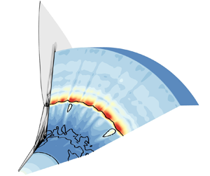
Figure 11 shows the contours of the azimuthal velocity perturbation w′ and pressure perturbation p′ corresponding to the least stable modes for the 0.33Re, 0.5Re and 0.75Re cases. The shock locations and dividing streamlines are superimposed. It is confirmed that these modes are of the same nature. In contrast to supersonic compression corner and double-wedge flows (Sidharth et al. Reference Sidharth, Dwivedi, Candler, & Nichols and W2018; Cao et al. Reference Cao, Hao, Klioutchnikov, Olivier and Wen2021; Hao et al. Reference Hao, Cao, Wen and Olivier2021), w′ is not confined in the separation region but also distributed in the inviscid regions behind the separation and curved shocks and in the supersonic jet. This may be attributed to the complexity of the shock interaction in the double-cone flows. The pressure perturbations further highlight the strong coupling between the separation region, separation and curved shocks and wave reflection in the supersonic jet. Similar observations were made by Tumuklu et al. (Reference Tumuklu, Theofilis and Levin2018). However, they only conducted axisymmetric GSA and thus found no unstable modes. As the Reynolds number is increased, the pressure perturbation in the supersonic jet penetrates the subsonic region bounded by the curved shock and slip line.

Figure 11. Contours of (a) the azimuthal velocity perturbation and (b) the pressure perturbation for different Reynolds numbers superimposed with shock locations and dividing streamlines. The contour levels are evenly spaced between ±0.5 of the maximum |w′| and between ±0.1 of the maximum |p′|.
For the highest Reynolds number, the flow is strongly destabilized. The growth rates and angular frequencies of the most unstable modes are plotted in figure 12 as a function of m. Note that mode 3 belongs to the same family as those shown in figure 10. The most unstable azimuthal wavenumber of mode 3 further decreases to 5. Meanwhile, a stationary mode (mode 1) and an oscillating mode (mode 2) occur with the growth rates peaking at m = 33 and 30, respectively. The frequency of mode 2 at m = 30 is approximately f = 4.8 kHz ( fL/u ∞ = 0.18), which belongs to the low-frequency regime. Modes 4 and 5 are also oscillating modes with even lower frequencies; however, these modes should be trivial due to the low growth rates.

Figure 12. Variations in (a) the growth rates and (b) the angular frequencies of the most unstable modes as a function of azimuthal wavenumber for the baseline case.
The azimuthal velocity perturbation and pressure perturbation contours are shown in figure 13 for modes 1‒3 at m = 33, 30 and 5. Modes 1‒3 structurally resemble the dominant stationary and oscillating unstable modes found in supersonic double-wedge and compression corner flows (Sidharth et al. Reference Sidharth, Dwivedi, Candler, & Nichols and W2018; Hao et al. Reference Hao, Cao, Wen and Olivier2021), especially in the separation region. These unstable modes also originate from the separated flow; however, they can be decorated by a particular type of shock interaction. Note that only Edney's type VI interaction was considered by Sidharth et al. (Reference Sidharth, Dwivedi, Candler, & Nichols and W2018) and Hao et al. (Reference Hao, Cao, Wen and Olivier2021). Here, w′ and p′ are also distributed in the supersonic jet with alternating signs in accordance with the wave reflection therein. The eigenfunctions of mode 3 are similar to those shown in figure 11 but characterized by a closer link between the supersonic jet and curved shock. Interestingly, modes 1 and 3 are absent in the secondary bubble in contrast to mode 2.

Figure 13. Contours of (a) the azimuthal velocity perturbation and (b) the pressure perturbation for modes 1‒3 at m = 33, 30 and 5 for the baseline case superimposed with shock locations and dividing streamlines. The contour levels are evenly spaced between ±0.5 of the maximum |w′| and between ±0.1 of the maximum |p′|.
4.4. Direct numerical simulations
In this section, DNS are performed to verify the GSA results and reveal the three-dimensional flow structures by solving the complete Navier–Stokes equations (3.1). Here, only the supercritical baseline case (i.e. run 35) is considered, which supports two stationary and three oscillating unstable modes.
The computational grid is generated by rotating the medium grid (750 × 350) around the axis over an angle of 72° to make the DNS affordable. Hence, the azimuthal wavenumbers that can be numerically resolved must be integer multiples of 5. This azimuthal domain extent is chosen because the growth rates of mode 1 at m = 30 and 35 are close to the maximum value (see figure 12a). In addition, the growth rates of modes 2 and 3 peak at m = 30 and 5, respectively. Two hundred grid cells are used in the azimuthal direction, which achieves a grid size comparable to that in the streamwise direction near the peak heating. Part of the grid upstream of separation is cut off to remove the axial singularity. The inlet boundary conditions are specified using the axisymmetric profile at the same streamwise location. Periodic boundary conditions are applied to the azimuthal boundaries. The initial flow field is constructed by duplicating the base flow in the azimuthal direction. Note that no external or internal disturbances are introduced. Therefore, global instability is expected to arise from the numerical round-off error.
The three-dimensional simulation is performed using PHAROS with the same numerical schemes as described in § 3.2, except that a second-order implicit scheme (Peterson Reference Peterson2011) is utilized for time marching. The physical time step is set to 20 ns. An independence study verified that a smaller time step did not change the flow evolution. The simulation is run for a total physical time t = 14 ms (tu ∞/L = 373.8) to ensure a quasi-steady state and to fully resolve the low-frequency unsteadiness. The sampling frequency is 0.5 MHz for spectral analysis.
To quantitatively characterize the evolution of global instability, the root mean square of the azimuthal velocity at a given streamwise station is defined by
 \begin{equation}{\sigma _w} = \sqrt {\frac{1}{{{N_r}{N_\phi }}}\sum\limits_{j = 1}^{{N_r}} {\sum\limits_{k = 1}^{{N_\phi }} {{{\left( {\frac{w}{{{u_\infty }}}} \right)}^2}} } } ,\end{equation}
where Nr and Nϕ are the numbers of grid cells in the radial and azimuthal directions, respectively. The temporal history of σw at x/L = 0.98 near the corner is shown in figure 14. After the initialization, σw experiences exponential growth until tu ∞/L ≈ 70 and nonlinear saturation. After tu ∞/L ≈ 240, a quasi-steady state is established. The growth rate of σw in the linear stage agrees well with that of mode 1 at m = 30 represented by the dashed-dotted line.

Figure 14. Temporal history of the root mean square of the azimuthal velocity at x/L = 0.98. The slope of the dashed-dotted line equals the growth rate of mode 1 at m = 30.
Figure 15(a) shows the contour of the azimuthal velocity in a certain x–r plane (ϕ = 42.5°) at tu ∞/L = 53.4 in the mid-linear stage. The spatial structure is almost identical to that of mode 1 captured by the GSA (see figure 13a), which confirms that mode 1 dominates the linear growth of the three-dimensional perturbations. The contours of the azimuthal velocity are also plotted in two wall-normal slices extracted at x/L = 0.98 and 1.20 in figure 15(b). Note that slices 1 and 2 are located in the separation bubble and downstream of reattachment, respectively. An azimuthal periodicity with m = 30 can be seen.

Figure 15. Contours of the azimuthal velocity in (a) the x–r plane at ϕ = 42.5° and (b) two wall-normal slices extracted at x/L = 0.98 and 1.20 at tu ∞/L = 53.4.
Figure 16 shows the temporal history of the azimuthally averaged surface Stanton number at x/L = 1.10 near flow reattachment. The heat flux remains constant at the beginning and oscillates in the late linear stage, which marks the emergence of mode 2. As will be seen later, the steep increase in St at tu ∞/L ≈ 170 is caused by the enlargement of the separation region. A fast Fourier transformation is carried out from tu ∞/L = 0 to 80.1 with the resulting power spectral density (PSD) plotted in figure 17(a). The dominant non-dimensional frequency is consistent with that of mode 2 at m = 30. The PSD of the surface Stanton number signal in the quasi-steady stage from tu ∞/L = 240.3 to 373.8 is presented in figure 17(b), which exhibits a broad-band feature also centred at fL/u ∞ ≈ 0.18.

Figure 16. Temporal history of the azimuthally averaged surface Stanton number at x/L = 1.10.

Figure 17. Power spectral density of the azimuthally averaged surface Stanton number signal at x/L = 1.10 in two time intervals: (a) from tu ∞/L = 0 to 80.1 and (b) from tu ∞/L = 240.3 to 373.8.
Figure 18 presents the contours of the surface Stanton number at different time instants. Isolines of Cf = 0 are also plotted to indicate the separation regions. The separation and reattachment points obtained from the base-flow solution are marked by arrows. At tu ∞/L = 0, the contour is axisymmetric. At tu ∞/L = 77.4, the reattachment line of the primary bubble and the separation and reattachment lines of the secondary bubble become corrugated, accompanied by slight azimuthal variations in the heat flux. After tu ∞/L = 154.9, the secondary bubble is strongly distorted and eventually breaks up into several small bubbles. The separation line of the primary bubble remains largely unaffected by the three-dimensionality of the flow field downstream, whereas the reattachment line exhibits a zigzag pattern. Similar features were reported by Cao et al. (Reference Cao, Hao, Klioutchnikov, Olivier and Wen2021) in their DNS of hypersonic compression corner flows.

Figure 18. Contours of the surface Stanton number at (a) tu ∞/L = 0, (b) tu ∞/L = 77.4, (c) tu ∞/L = 154.9, (d) tu ∞/L = 240.3, (e) tu ∞/L = 293.7 and ( f) tu ∞/L = 347.1. Black solid lines, isolines of Cf = 0; arrows, locations of the separation and reattachment points of the primary bubble obtained from the base-flow solution.
In contrast to the compression corner flows, no streamwise streaks that can persist for some distance are found downstream of reattachment. Instead, the narrow annular region of the maximum heat flux fragments into azimuthally periodic peaks and valleys. Meanwhile, the size of the separation region slightly increases compared to the axisymmetric value between tu ∞/L = 154.9 and 240.3, which explains the sudden increase in St shown in figure 16.
To closely examine the three-dimensional flow structures near flow reattachment, figure 19(a) shows an enlarged view of the surface Stanton number contour superimposed with skin friction lines at tu ∞/L = 293.7. Two wall-normal slices are extracted at x/L = 1.06 and 1.16. The contours of the streamwise velocity in the two slices superimposed with in-plane streamlines are shown in figure 19(b). Note that the white lines indicate the locations of the slices and zero streamwise velocity. In slice 1 located upstream of reattachment and downstream of the corner, the shear layer of the separation region is distorted by the counter-rotating streamwise vortical structures that are confined in the reversed flow region. The corrugated shear layer reattaches on the second cone to form a zigzag reattachment line with a series of nodes and saddle points shifted in the streamwise direction. The heat flux peaks are located downstream of the nodes, whereas the heat flux valleys are associated with the saddle points. In slice 2 located downstream of reattachment, another corrugated shear layer can be seen, emanating from the triple point (see figure 4). There are no streamwise vortices in the supersonic jet and reattaching boundary layer, which explains the absence of streamwise heat flux streaks downstream of reattachment.

Figure 19. (a) Enlarged view of the contour of the surface Stanton number superimposed with skin friction lines. (b) Contours of the streamwise velocity in two wall-normal slices extracted at x/L = 1.06 and 1.16 superimposed with in-plane streamlines at tu ∞/L = 293.7.
The azimuthally averaged distributions of the surface pressure coefficient and Stanton number at tu ∞/L = 293.7 are plotted in figure 20 with the grey-shaded envelope bounded by the maximum and minimum values in the azimuthal direction. In general, the averaged DNS results agree well with the experimental and base-flow data. However, strong azimuthal variations in the heat flux exist, especially near flow reattachment, where the relative difference can be as high as 50% compared with the mean value.

Figure 20. Comparison between the azimuthally averaged distributions of (a) the surface pressure coefficient and (b) the Stanton number at tu ∞/L = 293.7 and the experimental and base-flow data. The grey-shaded envelope represents the range of azimuthal variations.
5. Conclusions
The hypersonic laminar flow over a canonical 25°–55° double cone is investigated using CFD and GSA with varying unit Reynolds numbers. For all cases, no self-sustained inviscid unsteadiness is found, which is consistent with the unsteadiness boundary proposed by Hornung et al. (Reference Hornung, Gollan and Jacobs2021). The axisymmetric CFD reveals that the separation region is always terminated by the transmitted shock emanating from the interaction between the oblique and curved shocks induced by the first and second cones. The behaviours of skin friction, surface pressure and surface heat flux within the separation region are similar to those found in supersonic shock-induced separated flow over many canonical configurations. Secondary separation occurs beneath the primary bubble when the Reynolds number is greater than a critical value. The numerical predictions of the surface pressure and heat flux agree well with the experimental measurements. The numerical data are interpreted using the classical triple-deck scaling with the axisymmetric effect accounted for by the Mangler transformation. The universal values of the scaled separation and plateau pressures and the critical value of the scaled deflection angle for the emergence of the secondary separation also hold for double-cone flows. Note that the free-stream Mach number and wall temperature ratio are fixed in this study. The entire parameter space remains to be explored.
At relatively low Reynolds numbers, a stationary mode is captured by the GSA, whose growth rate increases as the Reynolds number is increased. Beyond a critical value, the mode becomes unstable with respect to azimuthally periodic perturbations. Meanwhile, the azimuthal wavenumber corresponding to the peak growth rate decreases. This mode is confined in the separation region and widely distributed behind the separation and curved shocks and within the supersonic jet. The onset of global instability occurs immediately prior to the emergence of secondary separation, which indicates that the instability criterion established for supersonic double-wedge and compression corner flows can be directly applied to double-cone flows. As the Reynolds number is further increased, the unstable mode continues to be destabilized. Meanwhile, an additional stationary and a low-frequency oscillating mode appear and become dominant at much larger azimuthal wavenumbers. Although generally resembling those found in supersonic double-wedge and compression corner flows, the structures of these modes are further complicated by the strong shock interaction in the double-cone flows.
The GSA results are verified by DNS initialized from the base-flow solution for the baseline case with no external or internal disturbances. The DNS reveal that the double-cone flow is highly three-dimensional and unsteady with strong variations in the surface heat flux near flow reattachment. It is indicated that axisymmetric laminar simulations would be questionable under flow conditions that are far beyond the global stability boundary. However, the GSA provides little information on convective instabilities that may happen locally in the flow field, e.g. the first and second modes (Mack Reference Mack1975; Smith Reference Smith1989; Smith & Brown Reference Smith and Brown1990; Fedorov Reference Fedorov2011; Butler & Laurence Reference Butler and Laurence2021) and vortical disturbances (Paredes, Choudhari & Li Reference Paredes, Choudhari and Li2016; Dwivedi et al. Reference Dwivedi, Sidharth, Nichols, Candler and Jovanovic2019). Potential laminar–turbulent transition induced by global and convective instabilities in hypersonic double-cone flows will be addressed in a future study.
Funding
This work is supported by the Hong Kong Research Grants Council (no. 15206519 and no. 25203721) and the National Natural Science Foundation of China (no. 12102377).
Declaration of interests
The authors report no conflict of interest.


 Open access