


1. Introduction
The urbanisation process profoundly affects the urban boundary layer (UBL) due to impervious man-made structures that alter the aerodynamic and hydrothermal properties of the land surface. These changes affect mass, energy and momentum transfer with the overlying atmosphere, which are the main drivers of urban weather and climate variability. These exchange processes play a crucial role in applications related to urban climate (Oke Reference Oke1982; Oke et al. Reference Oke, Mills, Christen and Voogt2017), urban ecohydrology (Meili et al. Reference Meili2020), air quality (Fernando et al. Reference Fernando, Lee, Anderson, Princevac, Pardyjak and Grossman-Clarke2001), urban resilience (Gorlé, Garcia-Sanchez & Iaccarino Reference Gorlé, Garcia-Sanchez and Iaccarino2015) and public health (Lowe, Ebi & Forsberg Reference Lowe, Ebi and Forsberg2011), to name a few. The interaction between the urban environment and atmospheric turbulence regulates these exchanges over a broad continuum of scales, ranging from tens of metres over the roof of a building to the kilometre scale over an urban neighbourhood (Rotach Reference Rotach1993, Reference Rotach1999). Motivated by the need to address open challenges in these fields and improve our interaction with the environment, the past decades have seen significant efforts to advance our understanding and ability to model turbulent transport in urban settings.
Scientific discovery in the field of microscale meteorology has historically relied on three pillars: field observations (Rotach et al. Reference Rotach2005), wind-tunnel experiments (Barlow, Harman & Belcher Reference Barlow, Harman and Belcher2004) and numerical simulations (Coceal et al. Reference Coceal, Thomas, Castro and Belcher2006). This paradigm has provided useful insight into how urban morphology affects flow statistics in the UBL, but the alignment between findings from these three fields is not always optimal. An instance of this is where a range of values for the von Kármán constant  $\kappa$ have been proposed by different field measurements and laboratory studies, with values varying from 0.33 to 0.43. This is comprehensively documented by Andreas et al. (Reference Andreas, Claffy, Jordan, Fairall, Guest, Persson and Grachev2006). In addition, Philips, Rossi & Iaccarino (Reference Philips, Rossi and Iaccarino2013) have pointed out several challenges in matching parameters of the underlying system, which hinder the accurate alignment of experimental data with numerical simulations. One such obstacle is the use of different methods to compute the repeating parameters, such as friction velocity, which cannot be uniformly applied across different fields. They also demonstrate that the vertical profile of the experimental data can often be accurately matched up to a certain height above the ground, beyond which significant deviations occur. This partial matching approach has also been utilised in other research studies (see, e.g., Coceal et al. Reference Coceal, Dobre, Thomas and Belcher2007; Xie, Coceal & Castro Reference Xie, Coceal and Castro2008), which serves to delimit the region of interest. Another factor contributing to the discrepancy between profiles is the sensitivity of flow statistics to changes in initial and boundary conditions and input parameters. This phenomenon often makes it challenging to establish connections between research findings within the same field (see, e.g., Wang et al. Reference Wang, Bou-Zeid, Au and Smith2011).
In the context of numerical simulations, direct numerical simulations (DNS) and large eddy simulations (LES) of open channel flow over surface-mounted cuboids have been the workhorse for studying turbulent transport in the UBL (Coceal et al. Reference Coceal, Thomas, Castro and Belcher2006; Xie & Castro Reference Xie and Castro2006; Leonardi & Castro Reference Leonardi and Castro2010; Claus et al. Reference Claus, Coceal, Thomas, Branford, Belcher and Castro2012; Yang & Anderson Reference Yang and Anderson2017; Schmid et al. Reference Schmid, Lawrence, Parlange and Giometto2019; Stroh et al. Reference Stroh, Schäfer, Frohnapfel and Forooghi2020). In these simulations, in addition to the aforementioned sources of discrepancies, one crucial factor affecting the accuracy and reliability of model results is the selection of the numerical domain size (Moin & Kim Reference Moin and Kim1982; Lozano-Durán & Jiménez Reference Lozano-Durán and Jiménez2014). Wall-bounded turbulence is characterised by coherent structures with a high correlation in the streamwise direction and a lower but still non-negligible correlation in the cross-stream direction. Thus, excessive periodisation in the horizontal directions can compromise the accuracy with which these structures are captured (Moin & Kim Reference Moin and Kim1982). Furthermore, in real-world environments, the scale separation (SS) between the inversion layer and the height of the canopies is often significant and the presence of a free-slip top boundary condition too close to the surface may result in spurious effects encompassing the entire UBL. Hence, it is crucial to exercise caution during the simulation design stage to ensure the precise capturing of statistics in the region of interest.
Past DNS and LES have been conducted using a range of computational domains, whose size is typically dictated by the available computational resources (Coceal et al. Reference Coceal, Thomas, Castro and Belcher2006; Xie & Castro Reference Xie and Castro2006; Stroh et al. Reference Stroh, Schäfer, Frohnapfel and Forooghi2020). To facilitate the comparison of the various domain sizes used, the concept of aspect ratio and SS is employed in this study. The naming convention used to describe the dimensions of the computational domain is graphically illustrated in figure 1(a,b), with the subscripts 1, 2 and 3 referring to the streamwise, cross-stream and vertical directions, respectively. The aspect ratio of a three-dimensional computational domain is defined as  $L_1/L_3:L_2/L_3:1$, where $L_1/L_3$ defines the streamwise aspect ratio (XAR) and $L_2/L_3$ defines the cross-stream aspect ratio (YAR). In addition, the height of the domain is described in terms of the SS, defined as $L_3/h$, where $h$ is the mean height of the underlying surface topography.

Figure 1. (a) Side view and (b) top view of the computational domain. (c) Marks the regions defined as urban canopy layer (UCL), upper roughness sublayer (URSL) and the outer layer (OL).
One of the early DNS studies of flow over cuboids was performed by Coceal et al. (Reference Coceal, Thomas, Castro and Belcher2006) to analyse turbulent flow statistics and unsteady effects in the roughness sublayer (RSL). This study represents a pivotal contribution to the understanding of canopy flow dynamics, achieved through the use of high-resolution DNS. However, as is common in such studies, the need for high resolution necessitated the selection of a smaller domain to ensure computational feasibility. For their open channel flow set-up, they used a numerical domain with an aspect ratio of  $1:1:1$ with an SS of 4. To showcase domain size independence, they compared selected statistics with a domain of aspect ratio $2:2:1$ and found the first-order statistics as well as second-order Reynolds stress $\overline {u^\prime _1 u^\prime _3}$ to match well. However, it is well known that the profile of $\overline {u^\prime _1 u^\prime _3}$ in the bulk of the flow is primarily determined by the imposed pressure gradient and has to vary linearly, as seen from the Navier–Stokes streamwise momentum balance equation; hence, the accurate collapse of $\overline {u^\prime _1 u^\prime _3}$ for domains with the same boundary layer height does not necessarily indicate the accurate capturing of other second-order moments. In addition, as the focus of this study was on the canopy configurations with high packing density, the domain used cannot be deemed as sufficient for the shown statistics to study RSL dynamics in general, as the extent of the RSL, as well as the turbulence characteristics of the RSL depend on the underlying surface configuration (Chung et al. Reference Chung, Hutchins, Schultz and Flack2021). Xie & Castro (Reference Xie and Castro2006) performed LES with domain $1:1:1$ and SS of 4 and found that their simulations were underpredicting the streamwise root-mean-square (r.m.s.) velocity $(u_{rms})$ when compared with corresponding DNS as well as experimental results. Later in this study (§ 3.1), it is shown that this underprediction is due to a direct consequence of limiting YAR of the domain and not due to differences between LES and DNS algorithms. Leonardi & Castro (Reference Leonardi and Castro2010) used various domain sizes with SS of 8 and aspect ratios ranging from $1:0.75:1$ to $1.25:1.25:1$ using DNS. The choice of XARs and YARs was purely driven by the need to accommodate a sufficient number of repeating patterns for different configurations. Schmid et al. (Reference Schmid, Lawrence, Parlange and Giometto2019) used a domain with SS of 4 and aspect ratio $1.5:1.5:1$ to study the effect of solid volume fraction on turbulent flow statistics using LES. Yang & Anderson (Reference Yang and Anderson2017) used LES to analyse the physics of roughness-induced secondary flows by using domains with SS of 15 and 20 while keeping the aspect ratio of the domain as ${\rm \pi} :{\rm \pi} :1$. They showcased that domain with aspect ratio $2{\rm \pi} :2{\rm \pi} :1$ produces similar results. However, this choice of high SS and high aspect ratio to reduce the artificial impacts of the numerical domain resulted in fewer nodes being used to resolve the cubes, which introduces an additional source of error. Stroh et al. (Reference Stroh, Schäfer, Frohnapfel and Forooghi2020) used DNS to study the polarity of secondary flows by using a domain with an SS of 23.25 and an aspect ratio of $8:4:1$. These studies demonstrate an apparent disparity in the employed domain sizes. From these observations, we infer the presence of a general trend towards maintaining a similar extent of the domain in both the streamwise and cross-stream directions. However, due to the asymmetrical nature of the turbulent flow structures and their extended presence in the streamwise direction compared to the cross-stream direction, it remains uncertain whether these domains will have an artificial effect on the flow statistics.
The presence of roughness-induced secondary flows, a topic which has received increased attention over the past decade (Willingham et al. Reference Willingham, Anderson, Christensen and Barros2014; Anderson, Li & Bou-Zeid Reference Anderson, Li and Bou-Zeid2015; Vanderwel & Ganapathisubramani Reference Vanderwel and Ganapathisubramani2015; Yang & Anderson Reference Yang and Anderson2017; Chung, Monty & Hutchins Reference Chung, Monty and Hutchins2018; Stroh et al. Reference Stroh, Schäfer, Frohnapfel and Forooghi2020; Wangsawijaya et al. Reference Wangsawijaya, Baidya, Chung, Marusic and Hutchins2020; Salesky, Calaf & Anderson Reference Salesky, Calaf and Anderson2022), also calls for special attention when designing the domain size. When the cross-stream spacing between the roughness elements is sufficiently large, it results in streamwise-aligned time-invariant counter-rotating vortices predominantly occupying the RSL. The size of these vortices is influenced by both the spacing of roughness elements in the cross-stream direction and the height of the domain. As demonstrated (see § 3.3), these circulations significantly affect the flow dynamics and necessitate a specialised approach to evaluate the effect of SS, as the height of the domain plays a critical role in governing these flows.
In the context of channel flow over aerodynamically smooth surfaces, analysis done by Comte-Bellot (Reference Comte-Bellot1963) and Schumann (Reference Schumann1973) guided early numerical studies to determine the optimal domain size to reduce the artificial impact of periodic boundary condition in the horizontal directions (Moin & Kim Reference Moin and Kim1982). Comte-Bellot (Reference Comte-Bellot1963) conducted two-point correlation measurements of velocity fluctuations and found that the correlation became negligible at a separation of  $3.2\delta$ in the streamwise direction and $1.6\delta$ in the cross-stream direction, where $\delta$ is the height of the half-channel. Schumann (Reference Schumann1973) and Moin & Kim (Reference Moin and Kim1982) later suggested that to reduce the artificial effect of periodic boundary conditions, the size of the simulation domain should be approximately twice as large as these dimensions. Lozano-Durán & Jiménez (Reference Lozano-Durán and Jiménez2014) conducted an extensive domain size analysis for plane channel flow using DNS at $Re_{\tau } = 4200$. They showed that the computational box with aspect ratio $2{\rm \pi} :{\rm \pi} :1$ was able to capture the one-point statistics with satisfactory accuracy. This aspect ratio of the domain aligns with the arguments provided by Schumann (Reference Schumann1973) and Moin & Kim (Reference Moin and Kim1982). Zheng, Montazeri & Blocken (Reference Zheng, Montazeri and Blocken2021) conducted a series of LES to examine the effect of domain size on pollutant dispersion in street canyons with periodic boundary conditions applied only in the cross-stream direction. The study recommends an SS of 7.5 with a width of at least $0.33L_3$, an upstream domain length of $0.67L_3$ and a downstream domain length of $1.33L_3$. These guidelines, however, are based on the 2.5-dimensional geometry of cross-stream-aligned bars and cannot be generalised to LES of open channel flow over cuboids or more general surface morphologies. As a result, there are currently no comprehensive guidelines for determining the appropriate size of the numerical domain for studying the UBL using an open channel flow set-up with LES.
The appropriateness of the domain size also depends on the specific region of interest under investigation. In the existing literature, it is commonly observed that researchers prefer smaller domain sizes when focusing on regions close to the surface, as capturing accurate statistics for the entire domain is not always necessary (Anderson Reference Anderson2016; Zhang et al. Reference Zhang, Zhu, Yang and Wan2022). In this study, we introduce the urban canopy layer (UCL), upper roughness sublayer (URSL) and outer layer (OL) as illustrated in figure 1(c) to facilitate the examination of flow statistics on a per-layer basis. Here, URSL is defined as a distinct component of the RSL, separate from the UCL, to avoid overlap when comparing flow statistics. Notably, we intentionally omit the inertial sublayer in our error analysis, as the study examines diverse packing densities and SS, where the presence of an inertial sublayer is not always guaranteed. We discuss this aspect in § 3.4. Hence, we incorporate the inertial sublayer, whenever present, in the OL for the purpose of our investigation.
This study investigates the effect of numerical domain size in these three distinct layers and addresses the aforementioned knowledge gap by providing extensive guidelines for researchers based on the packing density of the underlying configuration and the region of interest in a given study. The aim is to equip researchers with the essential data necessary for determining the optimal size of their numerical domain in LES of UBL flows, thereby allowing them to predict any changes to their statistical profiles that may occur due to limitations in domain size.
The structure of paper is organised as follows. Section 2 outlines the methodology employed in this study, which includes the details of the simulation algorithm (§ 2.1) and the dimensional analysis and simulation set-up (§ 2.2). The findings and observations from the simulations are presented in § 3. Finally, § 4 provides the conclusions drawn from the study.
2. Methodology
2.1. Simulation algorithm
A large suite of LES of flow over cuboid arrays is performed in this study using an in-house code (Albertson & Parlange Reference Albertson and Parlange1999a,Reference Albertson and Parlangeb; Bou-Zeid, Meneveau & Parlange Reference Bou-Zeid, Meneveau and Parlange2005; Chamecki, Meneveau & Parlange Reference Chamecki, Meneveau and Parlange2009; Anderson et al. Reference Anderson, Li and Bou-Zeid2015; Fang & Porté-Agel Reference Fang and Porté-Agel2015; Giometto et al. Reference Giometto, Christen, Meneveau, Fang, Krafczyk and Parlange2016; Li et al. Reference Li, Bou-Zeid, Anderson, Grimmond and Hultmark2016). The filtered Navier–Stokes equations are solved in their rotational form (Orszag & Pao Reference Orszag and Pao1975) to ensure the conservation of mass and kinetic energy in the inviscid limit, i.e.
 \begin{gather} \frac{\partial \tilde{u}_i}{\partial x_i}=0, \end{gather}
 \begin{gather}\frac{\partial \tilde{u}_i}{\partial t} + \tilde{u}_j \left(\frac{\partial \tilde{u}_i}{\partial x_j}-\frac{\partial \tilde{u}_j}{\partial x_i}\right) ={-} \frac{1}{\rho} \frac{\partial \tilde{p}^*}{ \partial x_i} - \frac{\partial \tau_{ij}^{SGS}}{\partial x_j} - \frac{1}{\rho }\frac{\partial \tilde{p}_\infty}{ \partial x_1} \delta_{i1}+\tilde{F}_i , \end{gather}
where  $\tilde {u}_1$, $\tilde {u}_2$, and $\tilde {u}_3$ are the filtered velocities along the streamwise $x_1$, cross-stream $x_2$, and wall-normal $x_3$ directions, respectively and $\rho$ is the reference density. The deviatoric component of the subgrid-scale (SGS) stress tensor ( $\tau _{ij}^{SGS}$) is evaluated via the Lagrangian scale-dependent dynamic (LASD) Smagorinsky model (Bou-Zeid et al. Reference Bou-Zeid, Meneveau and Parlange2005). Extensive validation of the LASD model has been carried out in both wall-modelled simulations of unsteady atmospheric boundary layer flow (Momen & Bou-Zeid Reference Momen and Bou-Zeid2017; Salesky, Chamecki & Bou-Zeid Reference Salesky, Chamecki and Bou-Zeid2017) and in simulations of flow over surface-resolved urban-like canopies (Anderson et al. Reference Anderson, Li and Bou-Zeid2015; Giometto et al. Reference Giometto, Christen, Meneveau, Fang, Krafczyk and Parlange2016; Li et al. Reference Li, Bou-Zeid, Anderson, Grimmond and Hultmark2016; Yang Reference Yang2016). Validation for the set-up used in this study is also given in Appendix A. Viscous stresses are neglected in the current study, and the skin friction is evaluated via an inviscid equilibrium logarithmic law of the wall for flow over aerodynamically rough surfaces (Giometto et al. Reference Giometto, Christen, Meneveau, Fang, Krafczyk and Parlange2016). Neglecting viscous stresses is valid under the assumption that SGS stress contributions are predominantly from the pressure field. Here, $\tilde {p}^*=\tilde {p}+\frac {1}{3}\rho \tau _{ii}^{SGS}+\frac {1}{2} \rho \tilde {u}_i \tilde {u}_i$ is the modified pressure, which accounts for the trace of SGS stress and resolved turbulent kinetic energy. The flow is driven by a spatially uniform pressure gradient. The magnitude of friction velocity $u_\tau$ is calculated based on imposed pressure gradient such that $(\boldsymbol {\nabla } p/\rho ) V_f = u^2_\tau A_s$, where $V_f$ is the volume of the fluid in the open channel and $A_s$ is the surface area. This allows the friction velocity to be an input parameter for this study. While different definitions of friction velocities are employed in the literature (Tian, Wan & Chen Reference Tian, Wan and Chen2023), we use the pressure-gradient-based definition of friction velocity in this study given its widespread usage in the open channel flow literature (Bou-Zeid, Meneveau & Parlange Reference Bou-Zeid, Meneveau and Parlange2004; Philips et al. Reference Philips, Rossi and Iaccarino2013; Fang & Porté-Agel Reference Fang and Porté-Agel2015; Yang & Anderson Reference Yang and Anderson2017; Stroh et al. Reference Stroh, Schäfer, Frohnapfel and Forooghi2020). The wall-parallel directions have periodic boundary condition, whereas the upper boundary has free-slip boundary condition, which can be expressed as $u_3=0, \partial u_1/ \partial x_3=0$ and $\partial u_2/ \partial x_3=0$. The lower surface represents an urban landscape with uniformly distributed cuboids. To resolve roughness elements, a discrete forcing immersed boundary method (IBM) is used (Mittal & Iaccarino Reference Mittal and Iaccarino2005; Chester, Meneveau & Parlange Reference Chester, Meneveau and Parlange2007; Giometto et al. Reference Giometto, Christen, Meneveau, Fang, Krafczyk and Parlange2016), where an artificial force $F_i$ is employed to bring the velocity to zero within the cuboids. An algebraic equilibrium wall-layer model, based on the law of the wall, is applied over a narrow band at the fluid–solid interface, i.e. on the surfaces of the cuboids, as well as on the solid base wall.
The spatial derivatives in the wall-parallel directions are computed by utilising a pseudo-spectral collocation method that relies on truncated Fourier expansions (Orszag Reference Orszag1970). Conversely, in the wall-normal direction, a second-order staggered finite difference scheme is implemented. The time integration process involves the adoption of a second-order Adams–Bashforth scheme. To deal with nonlinear advection terms, the  $3/2$ rule is utilised for de-aliasing (Canuto et al. Reference Canuto, Hussaini, Quarteroni and Zang2007; Margairaz et al. Reference Margairaz, Giometto, Parlange and Calaf2018). In addition, to ensure the enforcement of the incompressibility condition (2.1), a fractional-step method (Kim & Moin Reference Kim and Moin1985) is employed. The simulations are run for $200T$, where $T$ is the large eddy turnover time defined as $T = L_3/u_\tau$ to ensure temporal convergence of first- and second-order statistics. The time step employed in these simulations is selected to maintain a Courant–Friedrichs–Lewy (CFL) number below 0.1, ensuring numerical stability.
A large number of domain sizes are considered to study the impact of YAR, XAR and SS. The size of the computational domain is  $[0, L_1] \times [0, L_2] \times [0, L_3]$, with $L_3/h$ taking values $\{4, 8, 12, 16, 24\}$. We use $h$ to denote the height of cuboids, kept constant and equal to 1 across all simulations. Here $L_2/L_3$ takes values $\{1.5, 3.0, 4.5, 6.0\}$ while $L_1/L_3$ takes values $\{3.0, 6.0, 9.0, 18.0, 27.0\}$. An aerodynamic roughness length of $z_0 = 10^{-6}h$ is prescribed at the cube surfaces and the lower surface via the wall-layer model. With the chosen value of $z_0$, the SGS pressure drag is a negligible contributor to the overall momentum balance (Yang & Meneveau Reference Yang and Meneveau2016). The flow is in fully rough aerodynamic regime with a roughness Reynolds number $Re_\tau \equiv u_\tau h / \nu = 10^5$. The domain is discretised using a uniform Cartesian grid where each cube is resolved using $n_1 \times n_2 \times n_3 = 4 \times 4 \times 8$ for cases listed in tables 2 and 3, and $n_1 \times n_2 \times n_3 = 6 \times 6 \times 12$ for cases listed in tables 4 and 5, where $n_i$ denotes the number of collocation nodes per cube edge. In the case of lowest packing density accompanied by pronounced secondary flows, we have noted that the numerical instability of the compressed grid, necessary for boundary layer height-based scaling, has led to the generation of unrealistic flow patterns. Consequently, in our simulations involving packing density of 0.007 and SS of 4 and 8, we have utilised a grid resolution of $n_1 \times n_2 \times n_3 = 4 \times 4 \times 8$, as detailed in table 5. The error attributed to grid compression was notably lower compared with the errors observed in the statistics, thereby validating the appropriateness of employing grid compression for the analysis of cases scaled with boundary layer height-based scaling. The chosen grid resolution ensures that the study is computationally feasible while providing adequate resolution to capture the flow dynamics with large domains. The analysis presented in Appendices A and B shows that the chosen grid resolution yields flow statistics that are accurate up to second-order moments, based on the scope of this study.
2.2. Dimensional analysis and set-up of simulations
This subsection discusses the set-up of simulations and scaling arguments for flow statistics based on a Buckingham Pi theorem rationale. As mentioned in the introduction, the study aims to analyse the effect of domain geometry on flow statistics, with a lens on the YAR ( $L_2/L_3$), XAR ( $L_1/L_3$) and SS ( $L_3/h$) parameters. To achieve this objective, a suite of LES of flow over cuboid arrays is conducted, programmatically varying input parameters for the problem. Table 1 lists the quantities governing flow statistics; these quantities encompass two fundamental dimensions, length $L$ and time $T$, so the considered flow system can be completely characterised by a total of $11 - 2 = 9$ Pi groups (Buckingham Reference Buckingham1914).
Table 1. Variables determining flow characteristics for open channel flow simulations of flow over cuboids.

Based on the choice of repeating parameters, two different scaling relations can be obtained for the flow statistics. The merits and limitations of each are discussed in the following sections.
2.2.1. Canopy length-based scaling
In the canopy length-based scaling, the vertical height of cuboids ( $h$) and friction velocity ( $u_{\tau }$) are chosen as repeating parameters. While all length scales are normalised by $h$, special considerations are needed for $L_1$ and $L_2$ as the flow structures in the OL scale with the boundary layer height. By combining Pi groups, $L_1$ and $L_2$ can be scaled appropriately with $L_3$. Therefore, for example, the normalised mean streamwise velocity can be written in terms of non-dimensional groups as
 \begin{equation} U/u_{\tau} = f\left(\frac{L_3}{h}, \frac{L_2}{L_3}, \frac{L_1}{L_3}, \frac{h_2}{h}, \frac{h_1}{h}, \frac{s_2}{h}, \frac{s_1}{h}, \frac{x_3}{h}\right) . \end{equation}
 In order to study the effect of YAR ( $L_2/L_3$) on the non-dimensional mean streamwise velocity, the set of simulations in table 2 are chosen where for a particular packing density, only the non-dimensional group $L_2/L_3$ is varied across cases. This variation is achieved by varying the cross-stream length of the domain $L_2$ while keeping the boundary layer height $L_3$ constant. In order to minimise the effect of SS, the largest available value of $L_3$ across all the packing densities is chosen. All the simulations have $h_2/h=h_1/h=1$.
Table 2. Set of simulations to study the effect of YAR of the numerical domain on flow statistics. The Pi groups are mentioned in the table based on (2.3). For all the simulations,  $h_2/h = h_1/h = 1$.

A similar analysis is carried out to study the effect of XAR using the set of simulations in table 3. The variation in  $L_1/L_3$ is achieved by varying $L_1$ while keeping $L_3$ constant. Again, the largest value of SS ( $L_3/h$) across all the packing densities is chosen to minimise the effect of the blockage effect. While the largest $L_2/L_3$ among the available values is chosen for domains with $L_1/L_3 \geq 6$, $L_2/L_3 = 3.0$ is chosen for cases with $L_1/L_3 = 3$, since $3:3:1$ is a very common aspect ratio of the domain found in canopy flow literature.
Table 3. Set of simulations to study the effect of XAR of the numerical domain on flow statistics. The Pi groups are mentioned in the table based on (2.3). For all the simulations,  $h_2/h = h_1/h = 1$.

To study the effect of SS on flow statistics, set of simulations in table 4 are chosen where for a particular packing density, only  $L_3/h$ is varied across cases. This variation in $L_3/h$ was achieved by varying the boundary layer height $L_3$ while keeping the canopy height $h$ constant. It is later shown that $L_2/L_3 = 3$ and $L_1/L_3 = 6$ are large enough such that they do not artificially alter the flow statistics. Hence, these values are chosen while varying the SS.
Table 4. Set of simulations to study the effect of SS  $L_3/h$ of the numerical domain on flow statistics using canopy length-based scaling. The Pi groups are mentioned in the table based on (2.3). For all the simulations, $h_2/h = h_1/h = 1$.

2.2.2. Boundary layer height-based scaling
In boundary layer height-based scaling, the boundary layer height ( $L_3$) and friction velocity ( $u_{\tau }$) are chosen as repeating parameters. While all length scales are normalised by $L_3$, special considerations are needed for $h_1$ and $s_1$. As the displacement distance is determined by the extent to which flow can penetrate the canopy layer, the parameter is significantly influenced by the height of the roughness element ( $h$), gaps between two elements in the streamwise direction ( $s_1$) and the portion of the gap occupied by the roughness element ( $h_1$). Thus, to preserve the displacement distance, it is more appropriate to scale $s_1$ and $h_1$ with canopy height $h$, which can be achieved from a combination of the new set of Pi groups. In addition, the normalised parameter $h/L_3$ can be inverted to have a consistent SS definition throughout the paper.
Therefore, for example, the normalised streamwise velocity can be written in terms of non-dimensional groups as
 \begin{equation} U/u_{\tau} = f\left(\frac{L_3}{h}, \frac{L_2}{L_3}, \frac{L_1}{L_3}, \frac{h_2}{L_3}, \frac{h_1}{h}, \frac{s_2}{L_3}, \frac{s_1}{h}, \frac{x_3}{L_3}\right) . \end{equation}
 One may also choose to normalise  $h_1$ with $s_1$ and $h_2$ with $s_2$ to preserve the extent of roughness element in the repeating unit. The Pi groups presented in (2.4) ensure that the pairs ( $h_1, s_1$) and ( $h_2, s_2$) are normalised by the same length scale, $h$ and $L_3$, respectively. This automatically preserves $h_1/s_1$ and $h_2/s_2$ across cases, eliminating the need to modify these Pi groups further.
To study the effect of SS on flow statistics, a new set of simulations is proposed in table 5 based on boundary layer height-based scaling. Variation in  $L_3/h$ is achieved similarly by varying the boundary layer height $L_3$ while keeping the canopy height $h$ constant. For the cases with $L_3/h = 16$, surface geometry contains regularly arranged cubes. However, in order to preserve $h_2/L_3$ across different SS, the cross-stream extent of the cuboids $h_2$ must be adjusted, which results in distortion of the cube geometry. Therefore, as we decrease the domain height, the cuboids become slender in the cross-stream direction, while the streamwise extent of the cuboid remains the same, as it scales with the canopy height $h$. The motivation for implementing this scaling technique arises from the inadequacies of traditional canopy length-based scaling for canopy flows, which fails to isolate the effects of SS accurately. This alternative approach provides more precise isolation of SS effects across all packing densities, as explained in § 3.3 and shown in figure 11.
Table 5. Set of simulations to study the effect of SS  $L_3/h$ of the numerical domain on flow statistics using boundary layer height-based scaling. The Pi groups are mentioned in the table based on (2.4).

3. Results and observations
This section examines the effect of YAR, XAR and SS on selected turbulent flow statistics. Statistics are discussed on a per-layer basis for the three layers depicted in figure 1(c). To estimate the height of the RSL ( $x_{3r}$), we utilise a formula proposed by Chung et al. (Reference Chung, Hutchins, Schultz and Flack2021), i.e.
 \begin{equation} x_{3r} = \frac{s_2}{2} + d , \end{equation}
where  $d$ is the aerodynamic displacement height of the given surface. Values for $d$ are chosen from the values reported for square configurations in Kanda, Moriwaki & Kasamatsu (Reference Kanda, Moriwaki and Kasamatsu2004). This estimate is useful in predicting the extent of the RSL a priori; however, it tends to overestimate the height of RSL for densely packed configurations. For the purpose of our study, such shifts in the prediction of the extent of RSL have no significant impact on the error magnitudes, thus justifying the use of (3.1). In addition, an analysis of the existence of an inertial sublayer is also presented in this section for cases with varying SS and packing densities.
In this study, the operation of time-averaging is denoted by  $\overline {({\cdot })}$, while the process of spatial averaging in the horizontal directions is denoted by $\langle {\cdot }\rangle$. The averaging operation in the UCL is defined as a superficial average, where the flow statistics are normalised by the total volume, which includes the solid canopy elements (Schmid et al. Reference Schmid, Lawrence, Parlange and Giometto2019). A fluctuation from space and time-averaged quantity is denoted by the symbol $({\cdot })^\prime$. It is important to note that all the second-order statistics under discussion are computed using the resolved portion of the flow field. The present study does not include a detailed examination of SGS stresses. This decision is based on their limited contribution, comprising less than 2 % of the total Reynolds stress (Tian et al. Reference Tian, Wan and Chen2023). Moreover, given that SGS stresses arise from small-scale motions, it is anticipated that the influence of domain boundary conditions on these stresses will be of negligible significance.
3.1. Effect of YAR
This subsection discusses the impact of YAR on first- and second-order flow statistics as well as on the structure of turbulence through two-point correlation maps. To investigate the influence of YAR, simulations were conducted using three YAR values: 1.5, 3.0 and 4.5. These simulations were performed for four different packing densities, as outlined in table 2. In addition, for packing densities of 0.062 and 0.028, simulations were carried out with a YAR value of 6.0. The discrepancy between the profiles obtained with YAR 4.5 and YAR 6.0, concerning the first- and second-order statistics considered in this subsection, does not exceed 1 % across all layers. This satisfactory agreement between the results obtained using YAR 4.5 and YAR 6.0 suggests that the data derived from YAR 4.5 can confidently serve as the ground truth for the subsequent analysis presented in this subsection. Consequently, the following analysis exclusively focuses on the cases corresponding to YAR values of 1.5, 3.0 and 4.5.
Figure 2 shows profiles of mean streamwise velocity for different YAR values and packing densities. Differences in the profiles can be solely attributed to the artificial effects of the cross-stream width of the domain. Table 6 presents the error norms in different parts of the boundary layer. The results indicate that the velocity profile of the narrow domain (i.e. YAR 1.5) can estimate this quantity within 2 % error when compared with the velocity profile of the largest domain across all the layers and all the packing densities. Marginal improvements are seen in the error magnitudes when YAR is increased to 3.0.

Figure 2. Mean streamwise velocity profiles for different packing densities (a)  $0.25$, (b) $0.062$, (c) $0.028$ and (d) $0.007$. The vertical profiles for each packing density correspond to different YAR cases mentioned in table 2.
Table 6. Relative error ( $l_2$ norm) of mean streamwise velocity, resolved mean streamwise variance and resolved transverse integral length scale in UCL, URSL and OL for simulations with different YAR. Results from the largest domain (YAR 4.5) are considered as ground truths.

Figure 3 shows profiles of resolved mean streamwise variance for the same cases considered in figure 2 and errors in the different parts of the boundary layer are shown in table 6, which are also visualised in figure 4. It is observed that in UCL and URSL, the narrow domain is capable of predicting the resolved variance within 10 % of the largest domain, except for the case with packing density of 0.028, where the narrow domain results in a noticeable deviation in URSL, leading to an error of 17 %. In the OL, the error in this quantity exceeds 14 % for all cases except for the densely packed case, for which the error remains within 6 %. This observed error can be attributed to the tendency of the narrow domain to underestimate the value of variance. In contrast, the domain with YAR 3.0 can predict this quantity with an error magnitude that is approximately 7 % or lower when compared with the profiles of the largest domain across all the layers and all the packing densities, indicating a reduced influence of artificial periodisation in the cross-stream direction. This also indicates that the periodic boundary condition in the cross-stream direction has less of an effect on the first-order statistics compared with the second-order statistics. In order to investigate the underlying cause of the observed statistical shifts in the narrow domain, we now use two-point correlation to assess the effect of restricting cross-stream width of the domain on the topology of turbulence.

Figure 3. Resolved mean streamwise variance profiles for different packing densities (a)  $0.25$, (b) $0.062$, (c) $0.028$ and (d) $0.007$. The vertical profiles for each packing density correspond to different YAR cases mentioned in table 2.

Figure 4. Visualisation of error values in table 6 for different packing densities (a)  $0.25$, (b) $0.062$, (c) $0.028$ and (d) $0.007$. Error values for different layers are represented by distinct symbols: square, UCL; triangle, URSL; circle, OL.
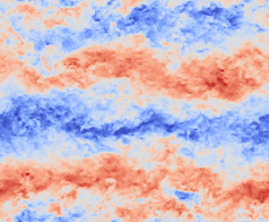
Figure 5 shows two-point correlation ( $R_{11}$) contours and instantaneous flow field fluctuations for different YAR at $x_3/L_3 = 0.6$. For brevity, only the cases with packing density of 0.028 are shown here. This packing density is chosen to qualitatively assess the reason behind the narrow domain noticeably underpredicting the resolved mean streamwise variance, as seen in figure 3(c). The colour bar is not shown here as the values are not used for inference; however, it is kept constant for all the flow field visualisations to get an appropriate sense of fast (red) and slow (blue) turbulent streaks. The two-point correlation between any two quantities is defined as
 \begin{equation} R_{\alpha \beta}(\Delta x_1,\Delta x_2,x_3)=\frac{\overline{u_\alpha^\prime(x_1, x_2, x_3) u_\beta^\prime(x_1+\Delta x_1, x_2+\Delta x_2, x_3)}}{\sigma_{u_\alpha}\sigma_{u_\beta}}, \end{equation}
where  $\sigma _{u_\alpha }$ is the standard deviation of the resolved fluctuating field $u^\prime _\alpha$. It is important to note that the presence of repeated indices in this context does not denote summation. From figure 5(a,c,e), we see that the streamwise extent of correlation for the narrow domain is much smaller compared with cases with YAR 3.0 and 4.5. This observation is strongly supported by the resolved streamwise instantaneous flow field fluctuations shown in figure 5(b,d,f). For the cases with YAR 3.0 and 4.5, we observe long streamwise turbulent structures of the order of the corresponding domain extent, justifying a more significant streamwise correlation. However, as shown in figure 5(b), no such structures are observed for the case with YAR 1.5. This shows that the narrow cross-stream width of the domain can significantly alter the growth of turbulent flow structures in the streamwise direction.

Figure 5. Two-point correlation  $R_{11}$ contours (a,c,e) and streamwise resolved instantaneous flow field fluctuations (b,d,f) for cases with packing density 0.028. The YAR is varied as: (a,b) 1.5; (c,d) 3.0; (e,f) 4.5. The wall-parallel slice shown in all the figures is taken at $x_3/L_3 = 0.6$.
As these coherent structures scale with the separation distance from the wall and as figure 5 only illustrates the case where  $x_3/L_3=0.6$, a more detailed analysis is needed to comment on the suitability of the domain with YAR 1.5 to accommodate a pair of these structures at different vertical positions and across all packing densities (Tomkins & Adrian Reference Tomkins and Adrian2003; Ganapathisubramani et al. Reference Ganapathisubramani, Hutchins, Hambleton, Longmire and Marusic2005; Coceal et al. Reference Coceal, Dobre, Thomas and Belcher2007). To address this matter, we analyse the typical width of such structures and investigate the ability of the domain with YAR 1.5 to accommodate fast and slow turbulent streaks at different vertical locations.
Figure 6 shows the total width of a fast and slow streak pair, which were observed in figure 5(d,f), as a function of height for cases with YAR 3.0 and 4.5. The width of a structure is computed as twice the cross-stream width over which  $R_{11}$ drops from 1 to 0. This width is then doubled to get the total width of the fast and slow streak pair. Figure 6 shows that as the size of streamwise coherent structure increases with height, the domain with YAR 1.5 is not sufficient to accommodate a pair of fast and slow streaks at $x_3/L_3 = 0.6$. This explains why no streamwise coherence was observed in figure 5(b). We also see that until $x_3/L_3 \approx 0.8$, the domain with YAR 3.0 is sufficient to accommodate a fast and slow streak pair even as the cross-stream extent of the domain is increased to YAR 4.5. A rapid increase in the structure size is observed beyond $x_3/L_3 \approx 0.8$ due to the free-slip boundary condition applied at the top of the computational domain, as it inhibits the inclined growth of the structures, conforming them to a planar configuration (Ganapathisubramani et al. Reference Ganapathisubramani, Hutchins, Hambleton, Longmire and Marusic2005). Since canopy flow studies in the open channel flow set-up do not typically focus on this region of the boundary layer, YAR 3.0 can be considered good enough to capture these coherent structures in the region below $x_3/L_3 \approx 0.8$. A noticeable deviation can be seen in the width of streamwise coherent structures between cases with YAR 3.0 and 4.5. However, as can be seen from figure 2, figure 3 and table 6, the effect of this deviation does not significantly alter the first- and second-order statistics. From figure 6, we also see that the vertical locations at which the width of the fast and slow streak pair exceeds the width of the domain with YAR 1.5 is different for different packing densities. For the case with highest packing density (i.e. 0.25), the crossing point lies at $x_3/L_3 \approx 0.37$. For packing densities 0.062 and 0.028, the crossing point lies at $x_3/L_3 \approx 0.15$, whereas this value is $x_3/L_3 \approx 0.07$ for packing density 0.007. Although these structures are seen to be increasing at a similar rate across all packing densities, the different vertical locations of these crossing points are a result of differences in the width of these structures near the top of the canopy layer. As observed by Coceal et al. (Reference Coceal, Dobre, Thomas and Belcher2007), the size of these structures near the canopy top is influenced by the geometry of obstacles, and their potential for growth depends on the configuration of said obstacles. This explains why different error magnitudes were observed in figure 3 across different packing densities for YAR 1.5, as the same domain width may or may not be able to accommodate these structures at a particular height based on the underlying surface configuration.

Figure 6. Width of turbulent streamwise coherent structures consisting of fast and slow streak pair. Cases with YAR of 4.5 are shown in solid lines and YAR of 3.0 in dashed lines. Colours correspond to different packing densities: 0.25, red; 0.062, green; 0.028, blue; 0.007, grey. Black vertical lines indicate the width of the domain: dash-dotted, YAR 1.5; dashed, YAR 3.0; solid, YAR 4.5. Purple horizontal line (dashed) indicates height of the UCL.
So far, the analysis has shown that insufficient cross-stream width of a numerical domain can inhibit the growth of streamwise coherent structures. To analyse the impact of YAR on the cross-stream coherent structures, resolved transverse integral length scale  $L_{22}$ is shown in figure 7 as a function of height. Errors in the profiles in different parts of the boundary layer are shown in table 6. The integral length scale in this study is defined as
 \begin{equation} L_{\alpha\alpha}(x_3) = \int_{0}^{\infty} R_{\alpha\alpha}(\Delta x_1 \delta_{\alpha 1}, \Delta x_2 \delta_{\alpha 2}, x_3)\,{\rm d} \Delta x_\alpha. \end{equation}
Thus,  $L_{22}$ characterises the length of instantaneous flow structures in the cross-stream direction. Note that the presence of repeated indices in this context does not imply summation. To discard the noise present around the correlation value 0, a cutoff value of 0.2 is used to compute the resolved transverse integral length scale (Ganapathisubramani et al. Reference Ganapathisubramani, Hutchins, Hambleton, Longmire and Marusic2005). The profile of the narrow domain in the OL exhibits significant deviation across all packing densities, as shown in figure 7, with errors exceeding 20 % in all cases. In UCL and URSL, a maximum of 7 % error is observed for the narrow domain. In contrast, the domain with YAR 3.0 is able to predict the length scale within 8 % of the values of the profiles with the largest domain across all the layers and packing densities, indicating a reduced influence of cross-stream periodisation on the spanwise growth of coherent structures. It is crucial to acknowledge that the two-point correlation function in the RSL cannot be considered independent of the position vector due to the heterogeneity of the flow field. In the RSL, strong signatures from the mean flow patterns affect the values of the integral length scale. Nevertheless, accepting this limitation permits the assessment of domain size impact in these layers based on the observed deviations since the mean flow patterns should have the same effect under identical surface configurations and flow conditions.

Figure 7. Resolved transverse integral length scale for different packing densities (a)  $0.25$, (b) $0.062$, (c) $0.028$ and (d) $0.007$. The vertical profiles for each packing density correspond to different YAR cases mentioned in table 2.
The extent of  $R_{22}$ is often used to see how far the flow field is correlated in the cross-stream direction. For the turbulent channel flow simulation, Moin & Kim (Reference Moin and Kim1982) showed that the transverse correlation becomes zero around $1.6L_3$ for a large domain. Based on this, they estimated that a cross-stream domain length of $3.2L_3$ is sufficient to accommodate coherent structures, which is in agreement with the presented results. However, the extent of transverse correlation does not always provide a complete picture. As shown in figure 5, the destruction of coherent structures for the narrow domain will also result in a decorrelated flow field, wrongly indicating the domain to be sufficient for decorrelation to occur.
3.2. Effect of XAR
This subsection discusses the effect of XAR of the numerical domain on first- and second-order flow statistics as well as on the structure of turbulence through two-point correlation maps.
Long structures seen in figure 5 are also a consequence of periodic boundary condition in the streamwise direction. In order to assess the effect of the interactions of these infinite structures, configurations mentioned in table 3 are simulated where the streamwise extent of the domain is varied systematically.
Figure 8 shows the resolved  $R_{11}$ correlation contours, mean streamwise velocity, resolved mean streamwise variance and resolved longitudinal integral length scale for cases with different XARs. For brevity, only the cases with packing density of 0.028 are shown here. From the figure, we see that as the domain is restricted in the streamwise direction, the correlation that infinite structures can sustain increases due to periodic boundary condition. Figure 8(a) shows that the infinite structure can sustain a positive correlation of 0.4 throughout the domain for the case with XAR 3.0. This value drops to 0.2 as the streamwise extent of the domain is increased, as shown in figure 8(c) for XAR 9.0. As the XAR is increased further to 27.0, the domain can no longer sustain a positive correlation of 0.2 at $x_3/L_3=0.6$ as shown in figure 8(e). The same is observed with negative correlation contours where the infinite structures can sustain a $-0.2$ correlation throughout the domain for cases with XAR 3.0 and 6.0, which is not observed for the case with XAR 9.0 and beyond. Figure 8(b,d,f) shows mean streamwise velocity and variance, as well as the integral length scale $L_{11}$, which characterises the length of instantaneous flow structures in the streamwise direction and is computed in accordance with (3.3), using a cutoff value of 0.5 (Ganapathisubramani et al. Reference Ganapathisubramani, Hutchins, Hambleton, Longmire and Marusic2005). The increased cutoff value, compared with the 0.2 used for $L_{22}$, ensures that all analysed cases, spanning various domains and packing densities, demonstrate a correlation value below the chosen contour threshold. From these statistics, we see that the strength of correlation resulting from periodisation influences the first- and second-order statistics. The cases with smaller streamwise extent tend to increase the correlation of the infinite structures throughout the domain, which coincides with increased resolved variance and slower mean streamwise velocity. The decrease in mean streamwise velocity is likely the result of increased turbulent mixing.

Figure 8. Two-point correlation  $R_{11}$ contours (a,c,e), mean streamwise velocity (b), resolved mean streamwise variance (d), resolved longitudinal integral length scale (f) for cases with packing density 0.028. The XAR is varied as: (a) 3.0, (c) 9.0 and (e) 27.0. The wall-parallel slice shown in (a,c,e) is taken at $x_3/L_3 = 0.6$. Domain configurations for cases with different XAR are presented in table 3.
The case with the shortest domain (i.e. XAR 3.0) was found to produce a mean streamwise velocity prediction that is within 4 % of the values obtained from the largest domain (i.e. XAR 27.0) across all layers and packing densities, as indicated by table 7. Figure 9 provides a visual representation of these error values. The maximum error observed in the resolved mean streamwise variance for the UCL and URSL remains limited to 6 % for all cases with the same domain. In contrast, the resolved mean streamwise variance error in the OL can increase up to 20 % for the shortest domain. On the other hand, the case with XAR 6.0 is able to predict both the statistics within 5 % of the values obtained from the largest domain across all the layers and packing densities, indicating a reduced influence of artificial periodisation on first- and second-order statistics. This also indicates that the periodic boundary condition in the streamwise direction has a less of an effect on the first-order statistics compared with the second-order statistics.
Table 7. Relative error ( $l_2$ norm) of mean streamwise velocity and resolved mean streamwise variance in UCL, URSL and OL for simulations with different XAR. Results from the largest domain (XAR 27.0) are considered as ground truths.


Figure 9. Visualisation of error values in table 7 for different packing densities (a)  $0.25$, (b) $0.062$ and (c) $0.028$. Error values for different layers are represented by distinct symbols: square, UCL; triangle, URSL; circle, OL.
It is interesting to note that the effect of a restricted streamwise and cross-stream domain extent on flow statistics is entirely the opposite. When the cross-stream width of the domain is restricted, it inhibits the growth of coherent structures, which can lead to lower variance and higher mean streamwise velocity. Conversely, when the streamwise length of the domain is restricted, it enhances the strength of coherent structures due to artificial periodisation, resulting in higher variance and lower mean streamwise velocity.
3.3. Effect of SS
This subsection discusses the effect of SS ( $L_3/h$) of the numerical domain on first- and second-order flow statistics. Here, two different scalings mentioned in §§ 2.2.1 and 2.2.2 are discussed in order to isolate the impact of SS appropriately.
Initially, simulation configurations are selected based on canopy length-based scaling discussed in § 2.2.1 to achieve different SS. The configurations are mentioned in table 4. This is the conventional way to test the effect of SS, where the domain height is varied systematically without changing the surface.
Figure 10 shows profiles of mean streamwise velocity for different SS and packing densities. For the case with the highest packing density shown in figure 10(a), all the velocity profiles from SS 8 to 16 collapse quite well. However, this trend is not observed when the packing density of the canopy surface is systematically decreased. Figure 10(b,c,d) shows significant deviation in the mean velocity profile when the SS varies from 8 to 16. This significant difference in the velocity profiles is observed for the sparsely packed cases because varying  $L_3/h$ while keeping $s_2/h$ constant changes a key parameter $s_2/L_3$, which controls the size and strength of secondary flows in sparse, regularly aligned canopies (Willingham et al. Reference Willingham, Anderson, Christensen and Barros2014; Vanderwel & Ganapathisubramani Reference Vanderwel and Ganapathisubramani2015; Yang & Anderson Reference Yang and Anderson2017). For example, when the domain height is decreased from $16h$ to $8h$ for the sparse configuration with packing density 0.007, for which $s_2/h$ is equal to 12, $s_2/L_3$ changes from 0.75 to 1.5. When $s_2/L_3$ is 0.75, it results in the generation of moderately strong secondary flows, whereas when the parameter is increased to 1.5, it results in strong secondary flows, which occupy the entire half-channel height. Figure 11 displays this effect. When the base configuration shown in figure 11(a) is scaled down using canopy length-based scaling, the resulting flow configuration shown in figure 11(b) is quite different. A dashed green line is drawn for reference at $x_3/h = 6.4$. We can clearly see that at this height, the flow configuration is entirely different, and the magnitude of this difference is directly related to the size and strength of secondary flows in the base configuration. Hence, the deviation observed in figure 10(b–d) cannot be solely attributed to the effect of SS. These results highlight that, for sparse configurations which induce secondary flows, the set of Pi groups stated in (2.3) cannot be used to isolate the effect of SS. For the densely packed case, the strength of the secondary flows is very weak due to the limiting cross-stream gap, and the surface essentially behaves as a conventional rough surface (Yang & Anderson Reference Yang and Anderson2017). This is why decreasing the parameter $s_2/L_3$ with increasing domain height does not have any effect on already weak secondary flows, which justifies the good collapse of streamwise velocity profiles observed in figure 10(a) across a large range of SS values.

Figure 10. Mean streamwise velocity profiles for different packing densities: (a) 0.25, (b) 0.062, (c) 0.028 and (d) 0.007. The vertical profiles for each packing density correspond to different SS cases mentioned in table 4.

Figure 11. Flow configuration for sparsely arranged canopies based on two different sets of Pi groups. The packing density of the surface is 0.007 in all cases. The SS is varied as (a) 16 and (b,c) 8. Configuration in (b) is scaled down from (a) based on canopy length-based scaling, whereas configuration in (c) is scaled down from (a) based on boundary layer height-based scaling. The green reference line matches  $x_3/h$ for (a,b) and $x_3/L_3$ for (a,c).
Considering the outcomes illustrated in figure 10(a), it becomes apparent that the influence of domain height on the mean velocity profile throughout the domain, via the generation of secondary flows, becomes negligible when the ratio  $s_2/L_3 \lesssim 0.25$. Thus, achieving converged mean velocity profiles appears feasible by adhering to the following SS criterion:
 \begin{equation} \frac{L_3}{h} \gtrsim 4 \frac{s_2}{h} . \end{equation}
Consequently, (3.4) postulates that in scenarios with a packing density of 0.062, where  $s_2/h=4$, the mean velocity profiles will converge satisfactorily beyond an SS value of 16. In contrast, for packing density 0.028, where $s_2/h=6$, deviations in the mean velocity profiles will persist even at an SS of 16. To test the validity of (3.4), two additional simulations are conducted with SS 24 for packing densities 0.062 and 0.028. The inference drawn from the equation aligns with the observations in figure 10(b,c), where the mean streamwise velocity profile with SS 16 is within 1 % of the profile with SS 24 for the packing density of 0.062. Meanwhile, for the packing density of 0.028, discrepancies in the velocity profile remain noticeable at both SS values of 16 and 24. Hence, (3.4) provides us with the means to make informed decisions regarding the appropriate SS level required to completely mitigate the effect of secondary flows on the mean velocity profiles.
Figure 12 depicts profiles of resolved mean streamwise variance for various SS and packing densities. The figure demonstrates that the rate of variance decay is significantly affected by the top boundary condition. Furthermore, the change in the parameter  $s_2/L_3$ also affects the variance values in the RSL. Yang & Anderson (Reference Yang and Anderson2017) showed that surfaces with $s_2/L_3$ considerably below 1 behave as conventional rough surfaces and exhibit weaker secondary circulations. Since the secondary flows are weak in such cases, the RSL statistics are predominantly affected by the wake flow from the canopies. Turbulence scales in the wake flow are primarily influenced by the dimensions of the canopy, which are preserved in canopy length-based scaling (Raupach, Antonia & Rajagopalan Reference Raupach, Antonia and Rajagopalan1991). As a result, the turbulence features of the RSL remain similar for these cases, enabling comparisons across different SS. Hence, this scaling can still be used to evaluate the effect of SS on RSL statistics for cases with packing densities of 0.25 and 0.062 and for SS where $s_2/L_3$ is less than or equal to 0.5. It is worth noting, however, that instances with $s_2/L_3 \approx 0.5$ also display minor secondary scale circulations, indicating that the RSL traits may not be identical, but these will not contribute significantly to the flow statistics. The error values of these cases in the UCL and URSL are presented in table 8 and visualised in figure 13. The maximum error observed for the mean streamwise velocity is less than 7 % across all SS. As for the resolved variance, the maximum error observed in the UCL is also less than 7 % across all SS. In the URSL, the cases with an SS of 12 capture this statistic with a maximum error of approximately 5 %, whereas the error can reach up to 15 % for the cases with an SS of 8 and 30 % for the case with an SS of 4. The discussion in the previous two paragraphs demonstrates that the canopy length-based scaling is unable to accurately isolate the effect of SS on turbulent flow statistics in the sparse cases which generate secondary flows as well as in the OL. Although scaling $x_3$ with $L_3$ instead of $h$ enables comparison of statistics in the OL for selected cases, it still does not facilitate comparison of the statistics for sparse cases or packing density 0.062 with SS 4. Thus, to overcome the limitations of canopy length-based scaling and to study the effect of SS across all the packing densities and the OL, a change in the repeating parameter determining the length scale is required.

Figure 12. Resolved mean streamwise variance profiles for different packing densities (a) 0.25, (b) 0.062, (c) 0.028 and (d) 0.007. The vertical profiles for each packing density correspond to different SS cases mentioned in table 4.
Table 8. Relative error ( $l_2$ norm) of mean streamwise velocity and resolved mean streamwise variance in UCL and URSL for simulations with different SS mentioned in table 4. Results from the domain with SS 16 are considered as ground truths.


Figure 13. Visualisation of error values in table 8 for different packing densities, (a)  $0.25$, (b) $0.062$. Error values for different layers are represented by distinct symbols: square – UCL, triangle – URSL.
A different scaling was proposed in § 2.2.2, where the domain height was chosen as a repeating parameter. This results in a different set of Pi groups presented in (2.4). The effect of this change in the repeating parameter can be appreciated in figure 11. When the base configuration shown in figure 11(a) is scaled down using boundary layer height-based scaling shown in figure 11(c), a similar flow configuration is achieved. A green dashed line is drawn for reference at  $x_3/L_3 = 0.4$, which accurately compares the extent of secondary circulation despite having different SS. Figure 11(c) also demonstrates that the underlying surface configuration changes and the cuboids become slender when the SS is decreased as per boundary layer height-based scaling. However, it should be noted that this change in configuration preserves the frontal area fraction of the surface, which results in a similar $z_0$ value throughout the cases for a fair comparison.
As the length scales of eddies in the RSL are predominantly associated with the canopy lengths, a direct comparison of statistics is not possible in this region, as the boundary layer height-based scaling distorts the surface. However, we can still compare statistics in the OL as it has turbulent eddies independent of canopy scales. In addition, the OL turbulence is most affected by the SS due to its close proximity to the no-stress boundary condition. Thus, minimising the effect of SS in the OL ensures that the effect of SS is minimal in UCL and URSL.
In order to accurately match equivalent points in the OL across cases, a new scaling is introduced, which maps the extent of the OL from 0 to 1. A non-dimensional function  $f(x_3, x_{3r}, L_3)$ is defined as
 \begin{equation} f(x_3, x_{3r}, L_3) = \frac{x_3 - x_{3r}}{L_3 - x_{3r}} , \end{equation}
where  $x_{3r}$ is the height of the RSL, which is calculated from (3.1).
Figure 14 shows the mean streamwise velocity defect for different SS and packing densities. Simulation set-ups for the shown cases can be found in table 5. A converging trend is observed across different packing densities, which was absent in figure 10. Figure 15 shows the resolved mean streamwise variance for the same cases. We observe that the errors between the streamwise velocity and resolved streamwise variance profiles presented in table 9 are relatively smaller for the densely packed case as well as the most sparse configuration considered in this study. Figure 16 provides a visual representation of these error values. A physical explanation for this behaviour can be provided by examining the characteristics of the RSL in the distorted surfaces. In canopy flows that do not generate secondary flows, the RSL is dynamically influenced by length scales associated with roughness elements (Raupach et al. Reference Raupach, Antonia and Rajagopalan1991). Therefore, the change in the dimensions of cuboids required to preserve the  $s_2/L_3$ Pi group changes the RSL characteristics of the surface. When the SS is low, the OL is not truly independent of influence from the roughness elements, and this change in the RSL turbulence also affects statistics in the OL. For the case with high packing density, the RSL does not extend significantly beyond the UCL, as can be inferred from the magnitude of dispersive fluxes (not shown), and OL independence is quickly achieved. In sparse canopies that generate secondary flows, the RSL is predominantly occupied by the counter-rotating vortices, which are preserved when the surface is scaled as per the boundary layer height-based scaling. Hence, the boundary layer height-based scaling tends to preserve the RSL characteristics for the sparse cases generating secondary flows. This explains the observed lower shift in streamwise velocity and resolved streamwise variance profiles for highly dense and highly sparse cases. From the table, we see that the domains with SS 12 predict both the quantities with less than 12 % error in the OL, and this error magnitude is likely to be lesser in UCL and URSL given their relatively more significant separation from the top boundary. In contrast the error for cases with SS 4 and 8 can be substantial and we refer the reader to table 9 for specific values. In addition, a monotonic increase is observed in the value of resolved variance as the SS is increased, except for the case with strong secondary flows. This shows that domains with smaller SS tend to inhibit the growth of turbulent structures, which contribute to the variance magnitude. This behaviour is clearly linked to the free-slip upper boundary condition, which is known to dampen velocity fluctuations, especially those in the vertical direction. In cases where strong secondary flows are present, the reversal in the trend indicates that the patterns of strong mean flow in the RSL affect the turbulence in the OL, leading to a higher variance value. However, when the SS is increased beyond 12, the statistics show excellent collapse, suggesting the recovery of OL independence.

Figure 14. Mean streamwise velocity defect profiles for different packing densities (a) 0.25, (b) 0.062, (c) 0.028 and (d) 0.007. The vertical profiles for each packing density correspond to different SS cases mentioned in table 5.

Figure 15. Resolved mean streamwise variance profiles for different packing densities (a) 0.25, (b) 0.062, (c) 0.028 and (d) 0.007. The vertical profiles for each packing density correspond to different SS cases mentioned in table 5.

Figure 16. Visualisation of error values in table 9 for different packing densities (a)  $0.25$, (b) $0.062$, (c) $0.028$ and (d) $0.007$. Circle represents error values in the OL.
Table 9. Relative error ( $l_2$ norm) of mean streamwise velocity and resolved mean streamwise variance for simulations with different SS and packing densities mentioned in table 5. Results from the case with the largest SS ( $L_3/h = 16$) are considered as ground truths. The statistics are compared in the OL.

3.4. Existence of inertial sublayer in canopy flows
In this subsection, the existence of an inertial sublayer is examined for cases with different SS available from the suite of simulations presented in table 4. In UBL flow, the inertial sublayer exists between the RSL and OL and is the region where most of the turbulent kinetic energy is generated (Jiménez Reference Jiménez2004). A logarithmic rise in the velocity within the region characterises this layer. In the flow over roughness elements, the logarithmic profile can be described in terms of aerodynamic roughness length  $z_0$, which quantifies the ability of the surface to absorb momentum, as
 \begin{equation} \frac{\langle\bar{u}_1\rangle}{u_\tau} = \frac{1}{\kappa} \ln\left(\frac{x_3 - d}{z_0}\right) , \end{equation}
where  $d$ is the aerodynamic displacement height of the given surface. As the existence of an inertial sublayer is not always guaranteed, we use a modified form of (3.6) in this study, as
 \begin{equation} \frac{\langle\bar{u}_1\rangle}{u_\tau} = \frac{1}{\kappa} \ln\left(\frac{x_3 - d}{L_3}\right) - \beta , \end{equation}
where  $\beta$ is a dimensionless constant defined as
 \begin{equation} \beta = \frac{1}{\kappa}\ln\left(\frac{z_0}{L_3}\right) . \end{equation}
 Figure 17 depicts the mean streamwise velocity across multiple cases with varying packing densities and SS in accordance with (3.7). In this study, the value of  $\kappa$ is chosen as 0.384 as recommended by Monkewitz, Chauhan & Nagib (Reference Monkewitz, Chauhan and Nagib2008). The solid black line in the figure serves as a reference to highlight the logarithmic profile of rough wall flow with a reference roughness length $z_{0_{ref}} = 0.25$ and $d=0$. The matching of slope of the profiles with the reference line indicates the existence of an inertial sublayer. The extent of deviation from the reference line depends on the magnitude of $z_0$. For the existence of logarithmic profiles, a layer sufficiently distant from the surface is necessary, such that the canopy scales do not affect the flow, and from the boundary layer height, such that $L_3$ is not a dominant length scale. Hence, SS becomes an essential parameter to determine whether the characteristics of the true inertial sublayer can be retrieved. In this study, an upper limit of $0.15L_3$ is considered for the inertial sublayer as beyond this height, the boundary layer height $L_3$ becomes a dominant scale (Jiménez Reference Jiménez2004; Marusic & Monty Reference Marusic and Monty2019). However, some researchers have recommended a larger value of $0.3L_3$ (Pope Reference Pope2000). The dashed lines in figure 17 indicate the upper limit of $0.15L_3$ for cases with $\lambda _p = 0.25$ and $0.062$, and the colours correspond to the velocity profiles. The solid horizontal lines represent the height of the canopy in these cases.

Figure 17. Mean streamwise velocity profiles for different SS (a) 16, (b) 12, (c) 8 and (d) 4. The vertical profiles for each SS correspond to different packing density cases mentioned in table 4. The horizontal lines correspond to the region between canopy height ( $x_3/h = 1$, solid) and the theoretical limit of the extent of inertial sublayer ( $x_3/L_3 = 0.15$, dashed) for packing densities 0.25 and 0.062.
Figure 17(a,b) shows that a logarithmic rise in the velocity is noticeable for cases with packing densities of  $0.25$ and $0.062$ and SS of 12 and 16. However, as the SS decreases to 8, the extent of the logarithmic layer is substantially reduced compared with the SS of 12 and 16. For this SS, the logarithmic rise is only observed for the case with a packing density of $0.25$ around the $0.15L_3$ mark. This occurs because the height extent of the RSL for a densely packed configuration (e.g. $\lambda _p = 0.25$) is smaller than that for configurations with relatively sparse arrangements (e.g. $\lambda _p = 0.062$), which can be observed from the extent to which the dispersive fluxes are significant (not shown). Hence, for the case with $\lambda _p = 0.25$, the extent of the RSL does not entirely occupy the significant portion of the region where the inertial sublayer can exist. However, the same is not true for the case with $\lambda _p = 0.062$. For cases with an SS of 4, the height of the canopy exceeds the upper limit of the extent of the inertial sublayer and, thus, the inertial sublayer is not observed for any case. For packing density 0.25 and 0.062 and SS 16, the corresponding $z_0$ values are measured at 0.068 and 0.086, respectively. Across different SS where the logarithmic profile is observed, the $z_0$ values remain within 0.5 % of those observed for SS 16.
Cases with packing densities of  $0.028$ and $0.007$ have been excluded from the discussion because these configurations generate secondary flows (see § 3.3). The size and strength of the secondary flows are significantly influenced by the height of the boundary layer, as $s_2/L_3$ is one of the crucial parameters governing secondary flows. Thus, for the cases with secondary flows, the height of the boundary layer $L_3$ directly affects the flow velocity in the RSL, which is occupied by the counter-rotating vortices. Consequently, if $L_3$ affects the velocity at the wall as well as near the top boundary, there is no layer in-between where the effect of $L_3$ on the velocity can be neglected. As a result, the basic requirement of independence from $L_3$ required for the existence of an inertial sublayer does not hold, and thus we do not observe an inertial sublayer for these cases in figure 17. This behaviour is consistent with findings from secondary flow research by Willingham et al. (Reference Willingham, Anderson, Christensen and Barros2014).
These findings highlight a crucial aspect of canopy flows, where the existence of an inertial sublayer is not solely determined by the SS as in the case of smooth wall flows but also depends on the packing density of the underlying surface. Figure 17 illustrates that, for a given SS, the inertial sublayer may or may not exist depending on the underlying canopy configuration. Specifically, for a densely packed configuration, the flow may exhibit an inertial sublayer, while a sparsely arranged canopy may not exhibit such a layer for a particular SS.
4. Conclusion
In this study, we have investigated the effect of numerical domain size on turbulent flow statistics for canopy flows spanning a wide range of packing densities. Specifically, we have considered the effect of three relevant length scales: YAR ( $L_2/L_3$), XAR ( $L_1/L_3$) and SS ( $L_3/h$). Furthermore, we have explored the question of the existence of an inertial sublayer for a wide range of cases with different packing densities and SS. Our findings reveal that poorly designed domains can have a significant effect on turbulent flow statistics and turbulent coherent structures. We outline the main findings of this study as follows.
(i) Effect of YAR ( $L_2/L_3$): narrower domains, characterised by YAR considerably below 3.0, can be inadequate to accommodate a pair of fast and slow turbulent streaks, thereby artificially destroying the growth of turbulent structures in the streamwise direction. In addition, a decrease in the growth of cross-stream structures is observed by analysing the resolved integral length scale $L_{22}$ in narrower domains. Moreover, the statistics indicate that narrower domains tend to underpredict the value of resolved streamwise variance across a wide range of packing densities. Overall, it is concluded that domains with YAR 3.0 or more are sufficient to reduce the artificial effect of cross-stream periodisation and to accurately capture the first- and second-order statistics. Detailed information about the specific errors in first- and second-order statistics in UCL, URSL and OL can be found in table 6.
(ii) Effect of XAR (
$L_1/L_3$): shorter domains, characterised by XAR considerably below 6.0, experience excessive periodisation, resulting in an artificial strengthening of the turbulent coherent structures in the streamwise direction. As a result, the coherent structures may exhibit longer correlation values throughout the domain. In addition, the statistics reveal that the shorter domains tend to overpredict the value of resolved streamwise variance across a wide range of packing densities. Overall, it is determined that domains with XAR 6.0 or more are sufficient to reduce the artificial effect of streamwise periodisation and to accurately capture the first- and second-order statistics. Detailed information about the specific errors in first- and second-order statistics in UCL, URSL and OL can be found in table 7.(iii) Effect of SS (
$L_3/h$): this study demonstrates that the conventional method to test the impact of SS has major limitations for canopy flows, especially for configurations where the parameter $s_2/L_3$ exceeds 0.5. To overcome the limitations of the existing method, a new set of Pi groups is proposed that can relatively accurately isolate the effects of SS. Using the novel $L_3$ scaling approach, we observe that domains with limited SS tend to underestimate the resolved variance values in the OL. In addition, our findings reveal that an SS of 12 and above is adequate to reduce the artificial effect of the top boundary condition on flow statistics in the UCL, the URSL and up to at least $0.6L_3$ in the OL. Detailed information about the specific errors in first- and second-order statistics can be found in tables 8 and 9.(iv) Existence of inertial sublayer: conventionally, SS is considered the sole parameter to determine the presence of an inertial sublayer in a flow field. However, our study shows that for canopy flows, the existence of an inertial sublayer depends not only on SS but also on the arrangement of the underlying surface. This is because the extent of the RSL depends on the underlying surface configuration and also because certain arrangements generate secondary flows which occupy the entire RSL. We found that for moderately dense (
$\lambda _p=0.062$) and dense ($\lambda _p=0.25$) cases, a logarithmic rise in the streamwise velocity profile could be recovered for SS of 12 and beyond. However, for an SS of 8, only the densely packed case ($\lambda _p=0.25$) exhibited the characteristic logarithmic rise. For sparse configurations which generate secondary flows, it is observed that the inertial sublayer does not exist for any SS. Scaling justification is provided in order to support the observed results for secondary flow cases.


Overall, our results indicate that a domain with an SS of 12 or larger, YAR of 3.0 or larger and XAR of 6.0 or larger is suitable for minimising the artificial effects of the numerical domain. However, researchers can use the error values reported in tables 6, 7, 8 and 9 to choose smaller domain than recommended based on their region of interest and research purpose. It is important to note that our study only considers the aligned configuration of canopy elements, but we expect our recommendations to be valid for staggered as well as other configurations based on the physical justifications provided in each subsections. We recommend that researchers match their configurations with an aligned configuration that has a similar extent of RSL.
Acknowledgements
The authors would like to thank Dr W. Li for his comments and suggestions on the manuscript. This work used the Anvil supercomputer at Purdue University through allocation ATM180022 from the Advanced Cyberinfrastructure Coordination Ecosystem: Services and Support (ACCESS) program, which is supported by National Science Foundation grants #2138259, #2138286, #2138307, #2137603 and #2138296. The authors also acknowledge the Texas Advanced Computing Center (TACC) at The University of Texas at Austin for providing high performance computing resources that have contributed to the research results reported within this paper.
Funding
This material is based upon work supported by, or in part by, the Army Research Laboratory and the Army Research Office under grant number W911NF-22-1-0178.
Declaration of interests
The authors report no conflict of interest.
Appendix A
In this section, we compare our LES results with independent DNS, LES and wind tunnel data to showcase validity of the results presented in this study. For this purpose, a staggered configuration with packing density 0.25 is simulated. The DNS results of Coceal et al. (Reference Coceal, Thomas, Castro and Belcher2006) with 32 nodes per cube (DNS_C32) and 64 nodes per cube (DNS_C64) are chosen, whereas the LES result of Anderson et al. (Reference Anderson, Li and Bou-Zeid2015) (LES_A) is chosen to perform the validation. Wind tunnel data from Cheng & Castro (Reference Cheng and Castro2002) (WT_CC) is chosen for the same configuration. The domain size chosen for this validation consists of SS 4, YAR 3 and XAR 6. The SS of 4 is chosen such that statistics in UCL, URSL and OL can be compared with DNS_C32, DNS_C64 and LES_A results using a single scaling. The choice of YAR and XAR is consistent with the recommendation of this study. We maintained a resolution of  $n_1 \times n_2 \times n_3 = 6 \times 6 \times 12$ per cube, mirroring the resolution employed in the study.
Figure 18 shows first- and second-order statistics for the chosen configuration. Here, friction velocity ( $u_\tau$) is based on the imposed pressure gradient in the LES, whereas the shear velocity ( $u_\ast$) for the LES results is obtained as
 \begin{equation} u_\ast{=} \sqrt{-\langle\overline{u^{\prime}_1 u^{\prime}_3}\rangle}_{{max}} . \end{equation}
Here, the symbol  $({\cdot })^{\prime }$ is used to denote temporal fluctuations. Note that the contribution from the subgrid stresses has been added in the second-order statistics and intrinsic averaging scheme as been used in UCL to match the statistics with Coceal et al. (Reference Coceal, Thomas, Castro and Belcher2006). This specific definition of shear velocity was adopted due to its consistency with both wind tunnel experiments and DNS data, a finding similarly reported by Tian et al. (Reference Tian, Wan and Chen2023). This relation gives $u_\ast =0.958u_\tau$ for the considered configuration.

Figure 18. (a) Mean streamwise velocity normalised by friction velocity ( $u_\tau$), (b) mean streamwise velocity normalised by shear velocity ( $u_\ast$), (c) r.m.s. value of streamwise Reynolds stress normalised by shear velocity ( $u_\ast$) and (d) r.m.s. value of Reynolds shear stress profile normalised by shear velocity ( $u_\ast$) for staggered arrangement with packing density 0.25. LES_A, LES result from Anderson et al. (Reference Anderson, Li and Bou-Zeid2015); DNS_C32/64, DNS result from Coceal et al. (Reference Coceal, Thomas, Castro and Belcher2006) using 32/64 nodes per cube; WT_CC, wind tunnel data from Cheng & Castro (Reference Cheng and Castro2002).
In conclusion, figure 18 demonstrates our LES algorithm's proficiency in capturing both first- and second-order statistics.
Appendix B
This section presents an analysis of the influence of grid resolution on turbulent flow statistics, specifically on streamwise velocity, resolved streamwise variance and resolved Reynolds shear stress. To conduct this study, a computational domain with SS of 4, YAR of 4.5 and XAR of 6.0 is selected. The domain is discretised with different resolutions such that  $n_1 \times n_2 \times n_3 = {4 \times 4 \times 8, 6 \times 6 \times 12, 8 \times 8 \times 16}$, where $n_i$ represents the number of collocation nodes per cube edge. Although this domain is not sufficient to accurately capture the turbulent flow statistics, the aim of this section is to demonstrate that the flow field is not significantly affected by the choice of grid resolution, indicating that the chosen domain is appropriate for this purpose. The results presented in figure 19 reveal that the resolutions of $4 \times 4 \times 8$ and $6 \times 6 \times 12$ can predict the trends in the profiles with satisfactory accuracy based on the scope of this work. The errors associated with these profiles are summarised in table 10. Error values are modest compared with corresponding variations in flow statistics resulting from XAR, YAR and SS. Since the existence of the inertial sublayer necessitates the accurate capture of flow statistics, a higher resolution of $6 \times 6 \times 12$ is selected for the analysis of the effect of SS in § 3.3. For §§ 3.1 and 3.2, a lower resolution of $4 \times 4 \times 8$ is chosen to ensure the computational feasibility of this study.

Figure 19. (a) Streamwise velocity, (b) resolved streamwise variance and (c) Reynolds shear stress profiles for a case with a packing density of  $0.028$, SS of $4$, and an aspect ratio of $1:4.5:6$, at different resolutions. The legend denotes the resolution as $(n_1, n_2, n_3)$, where $n_i$ represents the number of collocation nodes per cube edge.
Table 10. Relative error ( $l_2$ norm) of mean streamwise velocity, resolved mean streamwise variance and Reynolds shear stress for different resolutions. Results from the case with the highest resolution ( $8 \times 8 \times 16$) are considered to be ground truths.


 Open access