


1. Introduction
The evolution of turbulent kinetic energy in both physical and scale spaces is central to the understanding and prediction of turbulent flows. Significant progress was made over the past twenty years in the formulation of equations which govern this dual interscale and interspace turbulent kinetic energy evolution: Hill (Reference Hill1997, Reference Hill2001, Reference Hill2002) derived fully general two-point energy equations with/without Reynolds averaging which generalised the Kármán–Howarth equation to any turbulent flow (anisotropic and/or non-homogeneous) and which was first used for the analysis of non-homogeneous turbulence data by Marati, Casciola & Piva (Reference Marati, Casciola and Piva2004); Thiesset, Danaila & Antonia (Reference Thiesset, Danaila and Antonia2014) used a triple decomposition and derived two-point energy equations with terms which depend explicitly on large-scale coherent structures; and Larssen & Vassilicos (Reference Larssen and Vassilicos2023) applied a solenoidal/irrotational decomposition and adopted the procedure of Hill (Reference Hill2002) to derive solenoidal and irrotational two-point energy equations which they refer to as solenoidal and irrotational Kármán–Howarth–Monin–Hill (KHMH) equations.
In the case of statistically homogeneous and stationary forced turbulence, the average aspect of this evolution collapses into a simple balance between average interscale turbulence transfer rate and average turbulence dissipation rate in an intermediate range of scales bounded from below by the Taylor length and from above by an integral length scale. (The average two-point viscous diffusion rate is not negligible at scales below the Taylor length, see Appendix B of Valente & Vassilicos (Reference Valente and Vassilicos2015) and pp. 86–87 in Frisch (Reference Frisch1995).) Yasuda & Vassilicos (Reference Yasuda and Vassilicos2018) and Larssen & Vassilicos (Reference Larssen and Vassilicos2023) showed how unrepresentative this average balance is of what actually happens locally in space and time in this intermediate range of scales.
In the range of scales below the Taylor length, the average turbulent kinetic energy balance does not involve only interscale turbulence transfer and turbulence dissipation, but also viscous diffusion in scale space. Whilst the turbulent energy evolution and balance in the intermediate range is of paramount importance for reduced-order models and coarse graining, it is essential in the dissipative range for determining the smallest, viscosity-affected or dominated, local length and time scales. In the present study we investigate how representative the average turbulent kinetic energy balance is of what actually happens at length scales below the Taylor length in statistically stationary forced periodic turbulence. To this end, we use the recently developed solenoidal interscale and interspace turbulent kinetic energy equation (Larssen & Vassilicos Reference Larssen and Vassilicos2023) and a highly resolved direct numerical simulation (DNS) of forced Navier–Stokes turbulence with periodic boundary conditions in all three directions. For the average turbulent kinetic energy balance to be representative of the local (in space and time) turbulent kinetic energy balance, the fluctuations of each term in the local balance must be small compared with the non-zero average terms.
The following section describes our well-resolved DNS, the solenoidal and irrotational KHMH equations, and the spatiotemporal average forms of these equations for statistically homogeneous and stationary turbulence. Section 3 characterises the small-scale dynamics globally in terms of standard deviations, skewnesses, flatness factors and correlation coefficients. In § 4 we focus on energy transfer statistics conditioned on low and high two-point kinetic energy regions. We conclude in § 5.
2. The DNS, KHMH and average KHMH equations
We use the same DNS code used by Yasuda & Vassilicos (Reference Yasuda and Vassilicos2018) and Larssen & Vassilicos (Reference Larssen and Vassilicos2023) with the exact same negative damping forcing (McComb et al. Reference McComb, Linkmann, Berera, Yoffe and Jankauskas2015), and study a well-resolved DNS of statistically stationary turbulence that is periodic in all three directions with size  $512^3$ and kinematic viscosity
  $\nu =0.003$. The spatial resolution fluctuates between
  $k_{{max}}\eta =5.30$ and
  $5.79$ with standard deviation
  $0.11$ and average
  $k_{{max}}\langle \eta \rangle _{t} =5.50$ where
  $k_{{max}}$ is the highest resolved wavenumber,
  $\eta$ is the Kolmogorov length scale and
  $\langle \cdots \rangle _t$ denotes a time-average. The time-average Courant number is
  $\langle C \rangle _t=0.19$, the time-average Taylor length-based Reynolds number is
  $\langle Re_{\lambda } \rangle _t=81$ and the ratio of the box-size
  $2{\rm \pi}$ to the time-average integral length scale
  $\langle L\rangle _t$ equals
  $5.8$. The integral length scale is defined in terms of the three-dimensional energy spectrum
  $E(k,t)$ as
  $L(t)=(3{\rm \pi} /4)\int _{0}^{\infty }k^{-1}E(k,t)\,{\rm d}k/K(t)$, where
  $K(t)$ is the kinetic energy per unit mass. The ratio of the time-average Taylor length
  $\langle \lambda \rangle _t$ to
  $\langle L \rangle _t$ equals
  $2.6$. Statistics are sampled over 27 turnover times
  $T\equiv \langle L \rangle _t/\sqrt {2/3\langle K \rangle _t}$ with
  $T/10$ time intervals. The DNS resolution parameters are satisfactory for accurately assessing small-scale dynamics at low to moderate Reynolds number (Donzis, Yeung & Sreenivasan Reference Donzis, Yeung and Sreenivasan2008; Yeung, Sreenivasan & Pope Reference Yeung, Sreenivasan and Pope2018).
The KHMH equation governs the evolution of the velocity difference squared  $|\delta \boldsymbol {u}|^2$ across scales, space and time;
  $\delta \boldsymbol {u}=\delta \boldsymbol {u}(\boldsymbol {x},\boldsymbol {r},t) \equiv \boldsymbol {u}^{+}-\boldsymbol {u}^{-}$ denotes the velocity difference between fluctuating velocities
  $\boldsymbol {u}^{+}\equiv \boldsymbol {u}(\boldsymbol {x}^{+},t)$ and
  $\boldsymbol {u}^{-}\equiv \boldsymbol {u}(\boldsymbol {x}^{-},t)$ at locations
  $\boldsymbol {x}^{+}$ and
  $\boldsymbol {x}^{-}$, respectively, with centroid
  $\boldsymbol {x}=(\boldsymbol {x}^{+}+\boldsymbol {x}^{-})/2$ and separation vector
  $\boldsymbol {r}=\boldsymbol {x}^{+}-\boldsymbol {x}^{-}$,
  $\delta \boldsymbol {f}=\delta \boldsymbol {f}(\boldsymbol {x},\boldsymbol {r},t)$ is the body-force difference,
  $\delta p(\boldsymbol {x},\boldsymbol {r},t)$ is the pressure difference and
  $\rho$ is the density. The recently derived solenoidal and irrotational KHMH equations for statistically homogeneous/periodic turbulence (Larssen & Vassilicos Reference Larssen and Vassilicos2023) read (see Appendix A for summary of notation and some more information on each KHMH term)
 $$\begin{gather} \mathcal{A}_t +\mathcal{T}_{\bar{S}} + {\varPi}_{\bar{S}} = \mathcal{D}_{x,\nu} + \mathcal{D}_{r,\nu} - \mathcal{\epsilon} + \mathcal{I}, \end{gather}$$
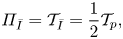 $$\begin{gather}{\varPi}_{\bar{I}} = \mathcal{T}_{\bar{I}} = \frac{1}{2}\mathcal{T}_p, \end{gather}$$
where  $\mathcal {A}_t\equiv \partial (|\delta \boldsymbol {u}|^2)/\partial t$ is the unsteadiness, or time-derivative, term;
  $\mathcal {D}_{r,\nu }=2 \nu \partial ^2 (|\delta \boldsymbol {u}|^2)/\partial r_k^2$ is the viscous diffusion in scale space;
  $\mathcal {D}_{x,\nu }\equiv \nu \partial ^2 (|\delta \boldsymbol {u}|^2/2)/\partial x_k^2$ is the viscous diffusion in physical space;
  $\mathcal {\epsilon } \equiv [2 \nu (\partial u_i^{+}/\partial x_k^{+} )^2+ 2 \nu (\partial u_i^{-}/\partial x_k^{-} )^2 ]$ is twice the sum of the pseudodissipation at
  $\boldsymbol {x}^{+}$ and
  $\boldsymbol {x}^{-}$;
  $\mathcal {I} \equiv 2\delta u_k \delta f_k$ is the energy input rate and
  $\mathcal {T}_p=-2\partial (\delta u_k \delta p/\rho ) /\partial x_k$ is the pressure-velocity term. For convenience, we also define the overall viscous diffusion and dissipation term
  $\mathcal {D}\equiv \mathcal {D}_{r,\nu }+\mathcal {D}_{x,\nu }-\mathcal {\epsilon }$. The solenoidal and irrotational interscale transfer terms read
  ${\varPi }_{\bar {S}}=2\delta \boldsymbol {u} \boldsymbol {\cdot } \boldsymbol {a}_{{\varPi }_{\bar {S}}}$ and
  ${\varPi }_{\bar {I}}=2\delta \boldsymbol {u} \boldsymbol {\cdot } \boldsymbol {a}_{{\varPi }_{\bar {I}}}$, where
  $\boldsymbol {a}_{{\varPi }_{\bar {S}}}$ and
  $\boldsymbol {a}_{{\varPi }_{\bar {I}}}$ are the solenoidal and irrotational components in centroid space
  $\boldsymbol {x}$ of the momentum interscale transfer rate
  $\boldsymbol {a}_{{\varPi }}=\delta \boldsymbol {u} \boldsymbol {\cdot } \boldsymbol {\nabla }_{\boldsymbol {r}} \delta \boldsymbol {u}$. Similarly, the solenoidal and irrotational transport terms read
  $\mathcal {T}_{\bar {S}}=2\delta \boldsymbol {u} \boldsymbol {\cdot } \boldsymbol {a}_{\mathcal {T}_{\bar {S}}}$ and
  $\mathcal {T}_{\bar {I}}=2\delta \boldsymbol {u} \boldsymbol {\cdot } \boldsymbol {a}_{\mathcal {T}_{\bar {I}}}$, where
  $\boldsymbol {a}_{\mathcal {T}_{\bar {S}}}$ and
  $\boldsymbol {a}_{\mathcal {T}_{\bar {I}}}$ are the solenoidal and irrotational components in centroid space of the momentum interscale transport rate
  $\boldsymbol {a}_{\mathcal {T}}=\tfrac {1}{2}(\boldsymbol {u}^{+}+\boldsymbol {u}^{-})\boldsymbol {\cdot } \boldsymbol {\nabla }_{\boldsymbol {x}} \delta \boldsymbol {u}$. Larssen & Vassilicos (Reference Larssen and Vassilicos2023) have shown that (2.1) follows from the integrated two-point vorticity equation and (2.2) follows from the integrated two-point Poisson equation for pressure. (More details on the Helmholtz decomposition applied to the equation for
  $\delta \boldsymbol {u}$ and the derivation of equations (2.1)–(2.2) can be found in Larssen & Vassilicos (Reference Larssen and Vassilicos2023). The nonlinear irrotational KHMH terms
  ${\varPi }_{\bar {I}}$ and
  $\mathcal {T}_{\bar {I}}$ are calculated here in terms of the pressure-velocity term (2.2). The solenoidal nonlinear KHMH terms
  ${\varPi }_{\bar {S}}$ and
  $\mathcal {T}_{\bar {S}}$ are obtained by first calculating
  ${\varPi }=2\delta \boldsymbol {u} \boldsymbol {\cdot } \boldsymbol {a}_{{\varPi }}$ and
  $\mathcal {T}=2\delta \boldsymbol {u} \boldsymbol {\cdot } \boldsymbol {a}_{\mathcal {T}}$ and then using
  ${\varPi }_{\bar {S}}={\varPi }-{\varPi }_{\bar {I}}$ and
  $\mathcal {T}_{\bar {S}}=\mathcal {T}-\mathcal {T}_{\bar {I}}$.)
The spatiotemporal average of the solenoidal KHMH equation for statistically stationary and homogeneous turbulence at scales small enough for a large-scale energy input rate  $\mathcal {I}$ to be negligible reads
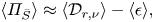 \begin{equation} \langle {\varPi}_{\bar{S}} \rangle \approx \langle \mathcal{D}_{r,\nu} \rangle - \langle \mathcal{\epsilon}\rangle, \end{equation}
where the angle brackets signify spatiotemporal averaging. As proven by Valente & Vassilicos (Reference Valente and Vassilicos2015) and confirmed by the DNS of Yasuda & Vassilicos (Reference Yasuda and Vassilicos2018) and Larssen & Vassilicos (Reference Larssen and Vassilicos2023),  $\langle \mathcal {D}_{r,\nu } \rangle$ is negligible at scales
  $r$ larger than the Taylor length. This average balance therefore simplifies to
  $\langle {\varPi }_{\bar {S}} \rangle \approx - \langle \mathcal {\epsilon }\rangle$ at scales larger than the Taylor length yet much smaller than the length scales where the large-scale forcing acts. It is this average balance that Larssen & Vassilicos (Reference Larssen and Vassilicos2023) showed to be non-representative of what actually happens in statistically stationary periodic turbulence. Here we concentrate on scales below the Taylor length and study how representative (2.3) is of what actually happens at these scales (locally in space and time). Viscous diffusion is therefore central to the present study.
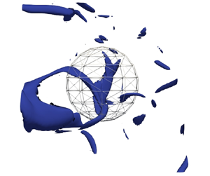
We calculate surface-averaged terms  $\mathcal {Q}^{a}(\boldsymbol {x},r_d,t)=({\rm \pi} r_d^2)^{-1}\iiint _{|\boldsymbol {r}|=r_d}Q(\boldsymbol {x},\boldsymbol {r},t)\,{\rm d}\boldsymbol {r}$ for every term
  $Q$ in the solenoidal KHMH equation (2.1) (in Appendix B we detail the surface-averaging scheme and show that the average and fluctuating residuals of the surface-averaged equation (2.1) are negligible). In figure 1 we plot the non-zero spatiotemporal averages of surface-averaged terms. At scales
  $\vert \boldsymbol {r} \vert = r_d < 0.6 \langle \lambda \rangle _t$, our DNS confirms (2.3) in the form
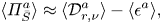 \begin{equation} \langle {\varPi}_{\bar{S}}^{a} \rangle \approx \langle \mathcal{D}_{r,\nu}^{a} \rangle - \langle \mathcal{\epsilon}^{a}\rangle, \end{equation}
and also shows that both sides of the equation are negative and that they tend to zero monotonically with decreasing  $r_d$. In fact, all terms in (2.1)–(2.2) tend to zero as
  $r_d$ tends to zero except
  $\mathcal {D}_{r,\nu }$ and
  $\mathcal {\epsilon }$. As clearly seen in figure 1,
  $\langle \mathcal {\epsilon }^{a}\rangle$ is independent of
  $r_d$ in statistically homogeneous/periodic turbulence. Note that a straightforward Taylor expansion of
  $\delta \boldsymbol {u}$ around
  $\boldsymbol {r}=0$ leads to
  $\lim _{r_{d}\to 0} \langle \mathcal {D}_{r,\nu }^{a} \rangle = \langle \mathcal {\epsilon }^{a}\rangle$. Figure 1 confirms that
  $\langle \mathcal {D}_{r,\nu }^a \rangle$ tends to
  $\langle \mathcal {\epsilon } \rangle ^a$ as
  $r_d$ tends to zero and also shows that
  $\langle \mathcal {D}_{r,\nu }^{a} \rangle$ is a positive monotonically decreasing function of
  $r_d$.
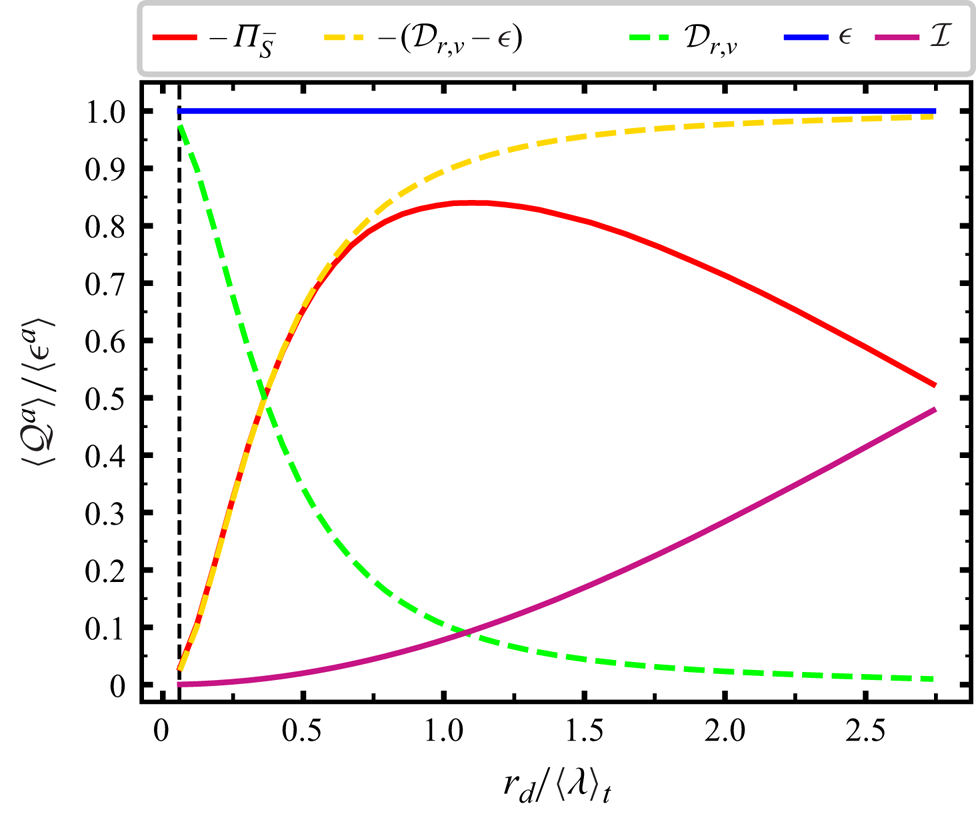
Figure 1. Non-zero spatiotemporal averages of surface-averaged terms of the solenoidal KHMH equation (2.1) as functions of  $r_{d}/\langle \lambda \rangle _t$. The vertical line marks the scale
  $r_d = \langle \eta \rangle _t$.
3. Fluctuating KHMH equation
The natural next step is to consider spatiotemporal fluctuations of the various terms in the KHMH equation around their average. By subtracting the spatiotemporal average solenoidal KHMH equation from the solenoidal KHMH equation we obtain
 \begin{equation} \mathcal{A}_t^a +\mathcal{T}_{\bar{S}}^a+{\varPi}_{\bar{S}}^{a'} \approx \mathcal{D}_{x,\nu}^{a} + \mathcal{D}_{r,\nu}^{a'} - \mathcal{\epsilon}^{a'}, \end{equation}
at scales  $r_d$ small enough for a large-scale energy input rate
  $\mathcal {I}$ to be negligibly small. In this equation we use the generic notation
  $\mathcal {Q}^{a'}=\mathcal {Q}^{a}-\langle \mathcal {Q}^{a}\rangle$ and we have taken into account the zero spatiotemporal averages of
  $\mathcal {A}_t^a$,
  $\mathcal {T}_{\bar {S}}^a$ and
  $\mathcal {D}_{x,\nu }^{a}$.
The focus of interest in this paper is the extent in which the average balance (2.4) is representative, i.e. the extent of validity of a local balance such as  ${\varPi }_{\bar {S}}^{a} \approx \mathcal {D}_{r,\nu }^{a} - \mathcal {\epsilon }^{a}$ at the smallest, dissipative, length-scales, that is length scales below
  $\approx 0.5 \langle \lambda \rangle _{t}$ where (2.4) holds well. The Reynolds number of our DNS (
 $\langle Re_{\lambda } \rangle _t=81$) may not be very high, but we are concerned with dynamics at scales between
  $r_{d}=\langle \eta \rangle _{t}$ and
  $r_{d}=\tfrac {1}{2}\langle \lambda \rangle _{t}$ which do not change much or change very slowly with increasing Reynolds number.
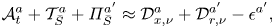
A natural starting point for addressing our question is in terms of standard deviations of the various terms in the fluctuating solenoidal KHMH equation (3.1). In figure 2(b,c) we plot these terms versus  $r_{d}/\langle \lambda \rangle _t$. To set the scene within a wider context, figure 2(a) shows how related standard deviations (surface averaged averages for direct comparison with Larssen & Vassilicos (Reference Larssen and Vassilicos2023) as opposed to statistics of surface averaged KHMH terms, see caption of figure 2) vary with
  $r_{d}/\langle \lambda \rangle _t$ over a range of scales
  $r_d$ that is wider than our actual range of interest as it is from
  $\langle \eta \rangle _t$ to
  $\langle L\rangle _{t} = 2.6 \langle \lambda \rangle _t$. In figure 2(b) we concentrate attention on the range
  $\langle \eta \rangle _t \le r_{d}\le 0.5 \langle \lambda \rangle _t$ (note the subtle difference between the quantities plotted in the vertical axes of figure 2a,b). It is clear that the standard deviations of all surface-averaged solenoidal KHMH terms except
  $\mathcal {D}_{r,\nu }^a$ and
  $\mathcal {\epsilon }^a$ tend to zero monotonically as
  $r_d$ decreases towards zero. The standard deviations of
  $\mathcal {D}_{r,\nu }^a$ and of
  $\mathcal {\epsilon }^a$ tend to the same non-zero value of approximately
  $1.2 \langle \mathcal {\epsilon }^a\rangle$ as
  $r_d$ decreases towards zero. Furthermore, the standard deviation of
  $\mathcal {D}_{r,\nu }^a - \mathcal {\epsilon }^a$ tends to zero in a way that is similar to the way that the standard deviation of
  ${\varPi }_{\bar {S}}^a$ tends to zero as
  $r_d$ tends to zero.
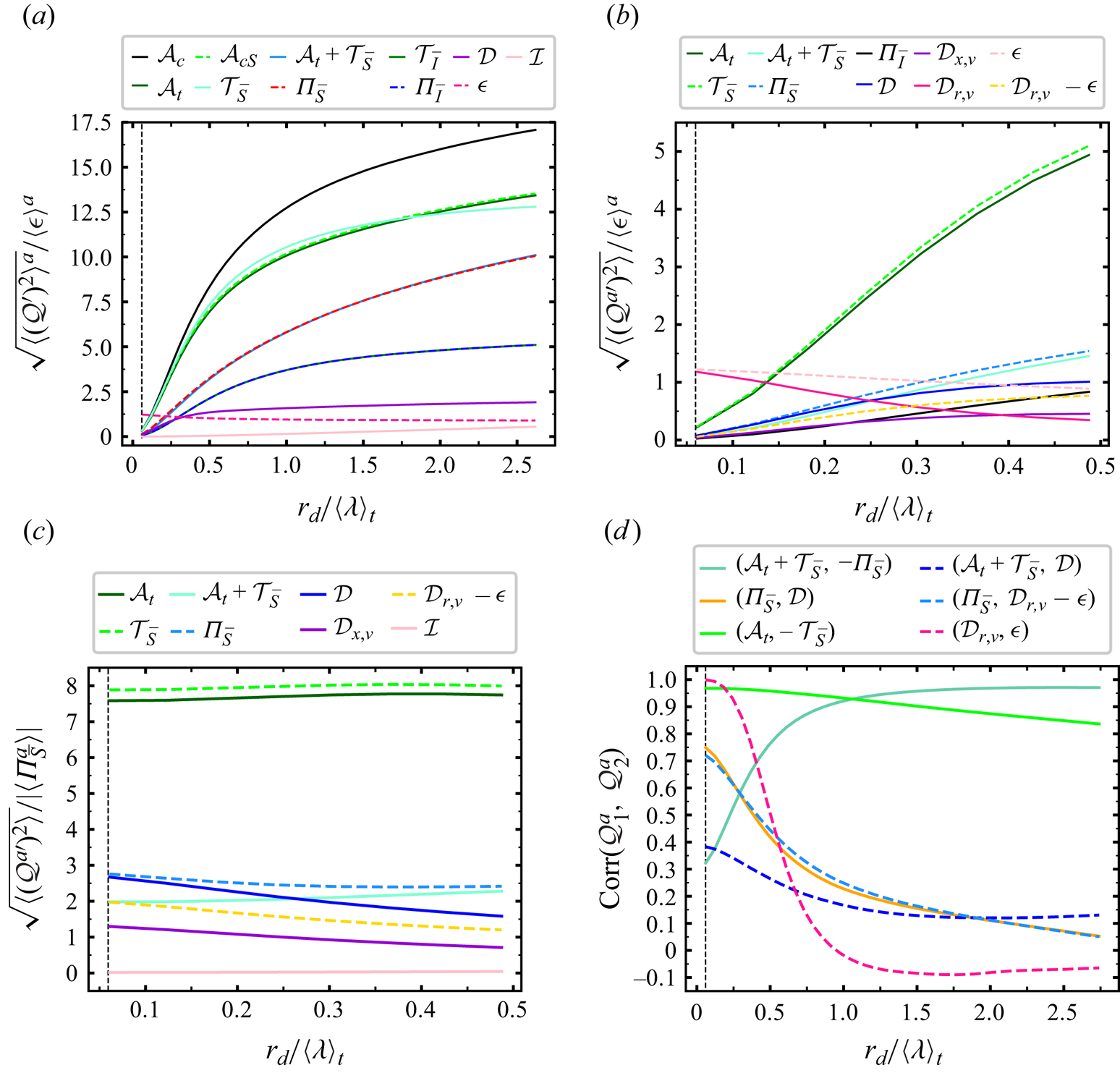
Figure 2. (a) Plot of  $\sqrt {\langle (\mathcal {Q}')^{2}\rangle ^{a}}$ normalised by
  $\langle \epsilon \rangle ^{a}$ which does not depend on
  $r_d$. This quantity is plotted versus
  $r_{d}/\langle \lambda \rangle _{t}$ for various terms
  $\mathcal {Q}$ in the solenoidal and irrotational KHMH equations, including
  $\mathcal {Q}= \mathcal {A}_{c} \equiv \mathcal {T}_{\bar {S}}+{\varPi }_{\bar {S}} + \mathcal {T}_{\bar {I}}+{\varPi }_{\bar {I}}$ and
  $\mathcal {Q}= \mathcal {A}_{c_S} \equiv \mathcal {T}_{\bar {S}}+{\varPi }_{\bar {S}}$ which are not discussed in the present paper but are included to allow checking by comparison with the corresponding plot in Larssen & Vassilicos (Reference Larssen and Vassilicos2023) obtained for a different DNS case. Note that the terms
  $\mathcal {A}_t+\mathcal {T}_{\bar {S}}$ and
  ${\varPi }_{\bar {S}}$ overlap and that the terms
  ${\varPi }_{\bar {I}}$ and
  $\mathcal {T}_{\bar {I}}$ also overlap. (b,c) Plots versus
  $r_{d}/\langle \lambda \rangle _{t}$ of normalised standard deviations of terms
  $\mathcal {Q}^{a}$ in the surface-averaged solenoidal KHMH equation (3.1); normalised by
  $\langle \epsilon \rangle ^{a}$ in (b) but normalised by
  $\vert \langle {\varPi }_{\bar {S}}^{a}\rangle \vert$ (which decreases with decreasing
  $r_d$) in (c). (d) Pearson correlation coefficients (obtained by averaging over space and time) of various spherically averaged terms in the solenoidal KHMH equation versus
  $r_{d}/\langle \lambda \rangle _{t}$.
For a proper initial estimate of the importance of fluctuations we need to compare these standard deviations with an appropriate non-zero spatiotemporal average. In figure 2(c) we plot them normalised by the absolute value of the spatiotemporal average of  ${\varPi }_{\bar {S}}^a$ which also tends to zero as
  $r_d$ tends to zero. The standard deviations of all the terms in the solenoidal KHMH equation which tend to zero as
  $r_d$ tends to zero do so at a rate that is comparable or even marginally slower than
  $\vert \langle {\varPi }_{\bar {S}}^a\rangle \vert$. In fact the standard deviation of
  ${\varPi }_{\bar {S}}^a$ is between 2.5 and 2.8 times larger than
  $\vert \langle {\varPi }_{\bar {S}}^a\rangle \vert$ for all
  $r_d$ in the range
  $\langle \eta \rangle _t$ to
  $0.5 \langle \lambda \rangle _{t}$ and the standard deviation of
  $\mathcal {D}_{r,\nu }^a - \mathcal {\epsilon }^a$ is between 1.2 and 2.0 times larger than
  $\vert \langle {\varPi }_{\bar {S}}^a\rangle \vert$ in that range. These fluctuations are clearly very significant compared with the average balance (2.4). Furthermore, whilst
  ${\varPi }_{\bar {S}}^a$ and
  $\mathcal {D}_{r,\nu }^a - \mathcal {\epsilon }^a$ are equal on average, the standard deviation of
  ${\varPi }_{\bar {S}}^a$ is at least 40 % larger than the standard deviation of
  $\mathcal {D}_{r,\nu }^a - \mathcal {\epsilon }^a$ in this range of scales.
Figure 2(c) also reveals that the largest fluctuations are by far those of  $\mathcal {A}_t^a$ and
  $\mathcal {T}_{\bar {S}}^a$ at these viscous length scales but that they cancel by the sweeping effect (discussed in some detail in Larssen & Vassilicos (Reference Larssen and Vassilicos2023)) so that the fluctuations of the Lagrangian transport
  $\mathcal {A}_t^a + \mathcal {T}_{\bar {S}}^a$ are between those of
  ${\varPi }_{\bar {S}}^a$ and
  $\mathcal {D}_{r,\nu }^a - \mathcal {\epsilon }^a$ in intensity (we use the term ‘Lagrangian transport’ in the sense that
  $\mathcal {A}_t^a + \mathcal {T}_{\bar {S}}^a$ can be interpreted as the rate of change of
  $\vert \delta \boldsymbol {u}\vert ^2$ in the frame moving with the mainly large-scale velocity
  $(\boldsymbol {u}^{+}+\boldsymbol {u}^{-})/2$). With the exception of the energy input rate which is insignificant at the very small scales, the smallest standard deviations are those of
  $\mathcal {D}_{x,\nu }^a$, the viscous diffusion rate in physical space. Pre-empting observations made later in this paper concerning the importance of
  $\mathcal {D}_{x,\nu }^a$, we note that the standard deviations of
  ${\varPi }_{\bar {S}}^{a}$ and
  $\mathcal {D}^{a} \equiv \mathcal {D}_{x,\nu }^{a} + \mathcal {D}_{r,\nu }^{a} - \mathcal {\epsilon }^{a}$ tend to equal each other as
  $r_d$ approaches
  $\langle \eta \rangle _t$ whereas the standard deviation of
  $\mathcal {D}_{r,\nu }^{a} - \mathcal {\epsilon }^{a}$ remains well below that of
  ${\varPi }_{\bar {S}}^{a}$.
The results of figure 2 are a first indication that the average balance (2.4) may not be characteristic of reality at the small scales where it holds. Not only are the standard deviations of  ${\varPi }_{\bar {S}}^{a}$ and
  $\mathcal {D}_{r,\nu }^{a} - \mathcal {\epsilon }^{a}$ much larger than their average values at scales
  $r_d$ under
  $0.5 \langle \lambda \rangle _t$, they are also the result of extremely intermittent fluctuations as evidenced by their flatness factors which are well over 40 at these scales (see figure 3b). In fact, all the terms in the solenoidal KHMH equation are much more intermittent than
  $\mathcal {\epsilon }^{a}$ and
  $\mathcal {D}_{r,\nu }^{a}$ at these scales, even
  $\mathcal {D}_{r,\nu }^{a} - \mathcal {\epsilon }^{a}$. Furthermore,
  ${\varPi }_{\bar {S}}^{a}$ and
  $\mathcal {D}_{r,\nu }^{a} - \mathcal {\epsilon }^{a}$ have significantly different skewnesses as shown in figure 3(a). With very intermittent fluctuations which are different in terms of standard deviations and skewnesses, it is likely that
  ${\varPi }_{\bar {S}}^{a}$ and
  $\mathcal {D}_{r,\nu }^{a} - \mathcal {\epsilon }^{a}$ are not typically equal. In fact, it is interesting to note the role of the viscous diffusion in physical space once again, given that the skewness of
  $\mathcal {D}^{a}$ is equal to the skewness of
  ${\varPi }_{\bar {S}}^{a}$ at scales
  $r_d$ between
  $\langle \eta \rangle _t$ and
  $0.25 \langle \lambda \rangle _t$.
Figure 3. Skewnesses (a) and flatness factors (b) of terms in the solenoidal KHMH equation across normalised scales  $r_{d}/\langle \lambda \rangle _t$. A point not made in the main text is that the only terms with increasing skewness as
  $r_d$ decreases towards
  $\langle \eta \rangle _t$ are
  $\mathcal {D}_{r,\nu }^{a}$ and
  $\mathcal {\epsilon }^{a}$.
The fluctuations of  ${\varPi }_{\bar {S}}^{a}$ and
  $\mathcal {D}_{r,\nu }^{a} - \mathcal {\epsilon }^{a}$ may be extremely intermittent and differ in magnitude, but be nevertheless correlated. The Pearson correlation coefficient of
  ${\varPi }_{\bar {S}}^{a}$ and
  $\mathcal {D}_{r,\nu }^{a} - \mathcal {\epsilon }^{a}$ is approximately 0.45 at
  $r_d = 0.5 \langle \lambda \rangle _t$ and increases to approximately 0.72 at
  $r_d = \langle \eta \rangle _t$ (see figure 2d). This is a significant correlation but the correlation curve between
  ${\varPi }_{\bar {S}}^{a}$ and
  $\mathcal {D}^{a}$ in figure 2(d) is approximately the same. It is important to note that two signals can be highly correlated yet be different nearly everywhere/everytime. Even so, the near-perfect correlation seen in figure 2(d) between
  $\mathcal {D}^a_{r,\nu }$ and
  $\mathcal {\epsilon }^a$ at scales close to
  $\langle \eta \rangle _t$ reflects very similar
  $\mathcal {D}^a_{r,\nu }$ and
  $\mathcal {\epsilon }^a$ spatiotemporal fields at
  $r_d$ close to
  $\langle \eta \rangle _t$ (the standard deviation of
  $1-\mathcal {D}^a_{r,\nu }/\mathcal {\epsilon }^{a}$ at
  $r_d = \langle \eta \rangle _t$ is 0.025). This is not inconsistent with the standard deviation and average of
  $\mathcal {D}^a_{r,\nu } - \mathcal {\epsilon }^a$ tending to 0 more or less together as
  $r_d$ decreases towards zero and with the skewness and flatness factors of the two fields being approximately the same at dissipative scales.
Given the high but far from perfect correlation between  ${\varPi }_{\bar {S}}^{a}$ and
  $\mathcal {D}_{r,\nu }^{a} - \mathcal {\epsilon }^{a}$ at scales close to
  $\langle \eta \rangle _t$ it may still not be a priori inconceivable that the average balance (2.4) might be, to some degree, a fairly representative balance even though the two spatiotemporal fluctuations of
  ${\varPi }_{\bar {S}}^{a}$ and
  $\mathcal {D}_{r,\nu }^{a} - \mathcal {\epsilon }^{a}$ differ significantly in fluctuation intensity and skewness. In the following section we investigate the degree of correspondence between
  ${\varPi }_{\bar {S}}^{a}$ and
  $\mathcal {D}_{r,\nu }^{a} - \mathcal {\epsilon }^{a}$ more closely by conditioning on low and high two-point kinetic energy
  $(\vert \delta \boldsymbol {u}\vert ^2 )^a$ for various small scales
  $r_d$ in the dissipative range below
  $\langle \lambda \rangle _{t}/2$ as these small-scale two-point energies reflect the smooth or near-singular local nature of the velocity field. Indeed, multifractal theories of turbulence (see Frisch (Reference Frisch1995)) associate local dissipative scales to varying levels of local near-singularities.
Given the results on  ${\varPi }_{\bar {S}}^{a}$ and
  $\mathcal {D}^{a}$ in figures 2 and 3 (same standard deviation and skewness at scales close to
  $\langle \eta \rangle _t$, similar flatness factors and correlations comparable to those of
  ${\varPi }_{\bar {S}}^{a}$ and
  $\mathcal {D}_{r,\nu }^{a} - \mathcal {\epsilon }^{a}$) we start by investigating the relation between
  ${\varPi }_{\bar {S}}^{a}$ and
  $\mathcal {D}^{a}$.
4. Small-scale dynamics in low and high energy regions
We define  $\langle \mathcal {Q} |(\vert \delta \boldsymbol {u}\vert ^{2})^a \rangle$ to be the average value of
  $\mathcal {Q}$ conditionally on
  $(\vert \delta \boldsymbol {u}\vert ^2 )^a$ being within a certain range of
  $(\vert \delta \boldsymbol {u}\vert ^2 )^a$ values and we consider 20 such ranges of increasing values of
  $(\vert \delta \boldsymbol {u}\vert ^2 )^a$: the
  $5\,\%$ smallest
  $(\vert \delta \boldsymbol {u}\vert ^2 )^a$ values, the
  $5\,\%$ to
  $10\,\%$ smallest
  $(\vert \delta \boldsymbol {u}\vert ^2 )^a$ values, and so on until the
  $95\,\%$ to
  $100\,\%$ smallest
  $(\vert \delta \boldsymbol {u}\vert ^2 )^a$ values which are actually the
  $5\,\%$ highest values of
  $(\vert \delta \boldsymbol {u}\vert ^2 )^a$ (given that the
  $100\,\%$ smallest
  $(\vert \delta \boldsymbol {u}\vert ^2 )^a$ values are by definition the totality of all values of
  $(\vert \delta \boldsymbol {u}\vert ^2 )^a$ for a certain
  $r_d$). In figure 4 we plot (figure 4a)
  $\langle \mathcal {D}^a | (\vert \delta \boldsymbol {u}\vert ^2 )^a \rangle$, (figure 4b)
  $\langle \mathcal {D}_{r,\nu }^{a} - \mathcal {\epsilon }^{a}| (\vert \delta \boldsymbol {u}\vert ^2 )^a \rangle$ and (figure 4c)
  $\langle \mathcal {D}_{x,\nu }^a | (\vert \delta \boldsymbol {u}\vert ^2 )^a \rangle$ versus
 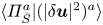 $\langle {\varPi }_{\bar {S}}^{a}|(\vert \delta \boldsymbol {u}\vert ^2 )^a\rangle$ for increasing
  $(\vert \delta \boldsymbol {u}\vert ^2 )^a$ and for scales
  $r_d$ between
  $\langle \eta \rangle _t$ and
  $\langle \lambda \rangle _t$. We checked that the results in this figure and in figure 7 with similar conditioning are insensitive to the number of
  $(\vert \delta \boldsymbol {u}\vert ^2 )^a$ ranges considered as we also tried
  $10$ and
  $100$ ranges with very similar results.
Figure 4. Plots of (a)  $\langle \mathcal {D}^{a} |(\vert \delta \boldsymbol {u}\vert ^{2})^a \rangle$, (b)
  $\langle \mathcal {D}_{r,\nu }^a-\mathcal {\epsilon }^a |(\vert \delta \boldsymbol {u}\vert ^{2})^a \rangle$ and (c)
  $\langle \mathcal {D}_{x,\nu }^a |(\vert \delta \boldsymbol {u}\vert ^{2})^a \rangle$ versus
  $\langle {\varPi }_{\bar {S}}^{a}|(\vert \delta \boldsymbol {u}\vert ^2 )^a\rangle$ (see the definition of these conditional averages in the first paragraph of § 4). All plotted quantities are normalised by
  $\vert \langle {\varPi }_{\bar {S}}^a\rangle \vert$ and are plotted for different values of
  $r_d$. The legend at the top of (a) gives the values of
  $r_{d}/\langle \lambda \rangle _t$ which correspond to different coloured symbols (note
  $\langle \eta \rangle _t \approx 0.06 \langle \lambda \rangle _t$). The average quantities plotted are conditional on 20 different ranges of
  $(\vert \delta \boldsymbol {u}\vert ^2 )^a$ values as described in the first paragraph of § 4 and ranges with increasing values of
  $(\vert \delta \boldsymbol {u}\vert ^2 )^a$ for each
  $r_d$ are from right to left in (a–c) (see the arrow indicating increasing local two-point energy
  $(\vert \delta \boldsymbol {u}\vert ^2 )^a$ in panel (a)).
Firstly, figure 4 shows that  $\langle \mathcal {D}^a | (\vert \delta \boldsymbol {u}\vert ^2 )^a \rangle$,
  $\langle \mathcal {D}_{r,\nu }^{a} - \mathcal {\epsilon }^{a}| (\vert \delta \boldsymbol {u}\vert ^2 )^a \rangle$,
  $\langle \mathcal {D}_{x,\nu }^a | (\vert \delta \boldsymbol {u}\vert ^2 )^a \rangle$ and
  $\langle {\varPi }_{\bar {S}}^{a}|(\vert \delta \boldsymbol {u}\vert ^2 )^a\rangle$ are all close to zero for the range of smallest values of
  $(\vert \delta \boldsymbol {u}\vert ^2 )^a$, i.e. the
  $5\,\%$ smallest
  $(\vert \delta \boldsymbol {u}\vert ^2 )^a$ values. As the
  $(\vert \delta \boldsymbol {u}\vert ^2 )^a$ values increase, the equality
  $\langle {\varPi }_{\bar {S}}^{a}|(\vert \delta \boldsymbol {u}\vert ^2 )^a\rangle \approx \langle \mathcal {D}^a | (\vert \delta \boldsymbol {u}\vert ^2 )^a \rangle$ appears clearly (see figure 4a) for all
  $r_d$ in the range
  $\langle \eta \rangle _{t} \le r_{d} \le 0.6 \langle \lambda \rangle _{t}$ whereas
  $\langle {\varPi }_{\bar {S}}^{a}|(\vert \delta \boldsymbol {u}\vert ^2 )^a\rangle \approx \langle \mathcal {D}_{r,\nu }^{a} - \mathcal {\epsilon }^{a}| (\vert \delta \boldsymbol {u}\vert ^2 )^a \rangle$ does not (see figure 4b). This behaviour has its root cause in the viscous diffusion in physical space which is non-zero in regions with high values of
  $(\vert \delta \boldsymbol {u}\vert ^2 )^a$. Interestingly,
  $\langle \mathcal {D}_{x,\nu }^a | (\vert \delta \boldsymbol {u}\vert ^2 )^a \rangle$ is increasingly negative as
  $(\vert \delta \boldsymbol {u}\vert ^2 )^a$ values increase (see figure 4c), which is also the case for all other three quantities plotted in figure 4. In fact both
  $\langle \mathcal {D}_{x,\nu }^a | (\vert \delta \boldsymbol {u}\vert ^2 )^a \rangle$ and
  $\langle \mathcal {D}_{r,\nu }^{a} - \mathcal {\epsilon }^{a}| (\vert \delta \boldsymbol {u}\vert ^2 )^a \rangle$ vary linearly with
  $\langle {\varPi }_{\bar {S}}^{a}|(\vert \delta \boldsymbol {u}\vert ^2 )^a\rangle$ if the
  $(\vert \delta \boldsymbol {u}\vert ^2 )^a$ values are not too small, and these two linear dependencies sum up to give
  $\langle {\varPi }_{\bar {S}}^{a}|(\vert \delta \boldsymbol {u}\vert ^2 )^a\rangle \approx \langle \mathcal {D}^a | (\vert \delta \boldsymbol {u}\vert ^2 )^a \rangle$.
We conclude that (i) with increasing  $(\vert \delta \boldsymbol {u}\vert ^2 )^a$ values, the average balance (2.4) is increasingly not representative of the conditionally averaged energy transfer balance at viscosity affected/dominated length scales and that (ii) the viscous diffusion in physical space cannot be neglected in regions of significant local inhomogeneity where
  $(\vert \delta \boldsymbol {u}\vert ^2 )^a$ is high. In such regions the viscous diffusion in physical space contributes to the loss of kinetic energy, though, on average, less than
  $\mathcal {D}_{r,\nu }^{a} - \mathcal {\epsilon }^{a}$ which is also negative on average but with higher magnitudes (see figure 4b,c).
The third conclusion is quantitative, namely that
 \begin{equation} \langle {\varPi}_{\bar{S}}^{a}|(\vert \delta \boldsymbol{u}\vert^2 )^a\rangle \approx \langle \mathcal{D}^a | (\vert \delta \boldsymbol{u}\vert^2 )^a \rangle \end{equation}
holds for all ranges of high enough  $(\vert \delta \boldsymbol {u}\vert ^2 )^a$ values in the range of scales
  $\langle \eta \rangle _{t} \le r_{d} \le 0.6 \langle \lambda \rangle _{t}$ whereas
  $\langle {\varPi }_{\bar {S}}^{a}|(\vert \delta \boldsymbol {u}\vert ^2 )^a\rangle = \langle \mathcal {D}_{r,\nu }^{a} - \mathcal {\epsilon }^{a}| (\vert \delta \boldsymbol {u}\vert ^2 )^a \rangle$ does not. This raises the question whether
  ${\varPi }_{\bar {S}}^{a} \approx \ \mathcal {D}^a$ happens more often than
  ${\varPi }_{\bar {S}}^{a} \approx \mathcal {D}_{r,\nu }^{a} - \mathcal {\epsilon }^{a}$ at these very small scales.
4.1. Probability density functions
To answer this question we plot in figure 5 probability density functions (p.d.f.s) of  ${\varPi }_{\bar {S}}^{a} -\mathcal {D}^a$ and
  ${\varPi }_{\bar {S}}^{a} - (\mathcal {D}_{r,\nu }^{a} - \mathcal {\epsilon }^{a})$ conditional on
  $(\vert \delta \boldsymbol {u}\vert ^2 )^a$. (This differs from Debue et al. (Reference Debue, Valori, Cuvier, Daviaud, Foucaut, Laval, Wiertel, Padilla and Dubrulle2021) who study separate p.d.f.s of interscale transfer rate – without solenoidal/irrotational decomposition – on the one hand and dissipation/viscous diffusion in scale space on the other.) The red curves are p.d.f.s conditional on the 5 % smallest values of
  $(\vert \delta \boldsymbol {u}\vert ^2 )^a$ whereas the blue and green curves are, respectively, p.d.f.s conditional on the 5 % and 0.5 % highest values of
  $(\vert \delta \boldsymbol {u}\vert ^2 )^a$ for a given length scale
  $r_d$. Figure 5(a,b) are for
  $r_{d}=\langle \eta \rangle _t$, figure 5(c,d) are for
  $r_{d}=0.24 \langle \lambda \rangle _t$ and figure 5(e, f) are for
  $r_{d}=0.48 \langle \lambda \rangle _t$. The first observation to make is that, if normalised by their maximum p.d.f. value,
  $P_{{max}}$ and the standard deviation of
  ${\varPi }_{\bar {S}}^{a}$ for high
  $(\vert \delta \boldsymbol {u}\vert ^2 )^a$ events, the high
  $(\vert \delta \boldsymbol {u}\vert ^2 )^a$ p.d.f.s of
  ${\varPi }_{\bar {S}}^{a} -\mathcal {D}^a$ (blue and green curves in figure 5a,c,e) are approximately symmetric with respect to positive and negative values and become decreasingly heavy tailed with decreasing
  $r_d$. Irrespective of the value of
  $r_d$ in the range
  $\langle \eta \rangle _{t}\le r_{d} \le 0.5 \langle \lambda \rangle _{t}$, the most likely value of
  ${\varPi }_{\bar {S}}^{a} -\mathcal {D}^a$ is zero at the 5 % and 0.5 % highest
  $(\vert \delta \boldsymbol {u}\vert ^2 )^a$ events. The most likely value of
  ${\varPi }_{\bar {S}}^{a} -\mathcal {D}^a$ is also zero at the 5 % lowest
  $(\vert \delta \boldsymbol {u}\vert ^2 )^a$ events. However, the p.d.f. of
  ${\varPi }_{\bar {S}}^{a} -\mathcal {D}^a$ conditional on these 5 % lowest
  $(\vert \delta \boldsymbol {u}\vert ^2 )^a$ events and normalised by
  $P_{{max}}$ and the standard deviation of
  ${\varPi }_{\bar {S}}^{a}$ for these events (red curves in figure 5a,c,e) becomes increasingly heavy tailed with decreasing
  $r_d$ in the range
  $\langle \eta \rangle _{t}\le r_{d} \le 0.5 \langle \lambda \rangle _{t}$ (but remains approximately symmetric with respect to positive and negative values).
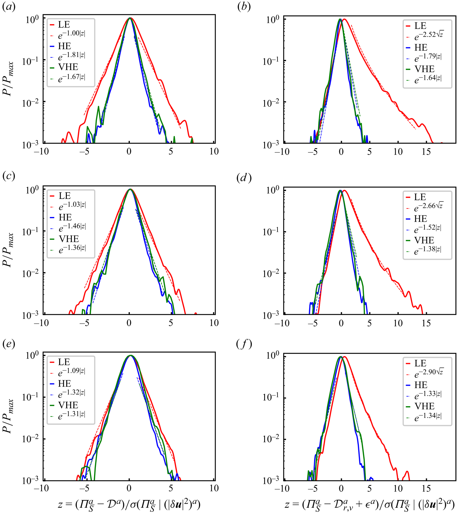
Figure 5. Probability density functions of  ${\varPi }_{\bar {S}}^a-\mathcal {D}^a$ (a,c,e) and
 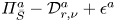 ${\varPi }_{\bar {S}}^a-\mathcal {D}_{r,\nu }^a+\mathcal {\epsilon }^a$ (b,d, f) conditional on low energy (LE) events (the events with the
  $5\,\%$ smallest
  $(|\delta \boldsymbol {u}|^2)^a$ values at scale
  $r_d$), high energy (HE) events (the events with the
  $5\,\%$ highest
  $(|\delta \boldsymbol {u}|^2)^a$ values at scale
  $r_d$) and very high energy (VHE) events (the events with the
  $0.5\,\%$ highest
  $(|\delta \boldsymbol {u}|^2)^a$ values at scale
  $r_d$): (a,b)
  $r_d = \langle \eta \rangle _t$; (c,d)
  $r_d = 0.24 \langle \lambda \rangle _t$; (e, f)
  $r_d=0.48 \langle \lambda \rangle _t$.
  $P_{{max}}$ and
  $\sigma ({\varPi }_{\bar {S}}^a \vert (|\delta \boldsymbol {u}|^2)^a)$ denote, respectively, the p.d.f. maximum value and standard deviation of
  ${\varPi }_{\bar {S}}^a$ conditional on the particular range of
  $(|\delta \boldsymbol {u}|^2)^a$ values considered. The dashed lines show exponential or stretched exponential fits of the p.d.f.s calculated with least squares.
Unlike  ${\varPi }_{\bar {S}}^{a} -\mathcal {D}^a$, the most likely value of
  ${\varPi }_{\bar {S}}^{a} - (\mathcal {D}_{r,\nu }^{a} - \mathcal {\epsilon }^{a})$ is not zero, see figure 5(b,d, f). It is non-zero and positive if conditioned on the 5 % lowest
  $(\vert \delta \boldsymbol {u}\vert ^2 )^a$ events, and non-zero and negative if conditioned on either the 5 % or the 0.5 % highest
  $(\vert \delta \boldsymbol {u}\vert ^2 )^a$ events. However, similarly to
  ${\varPi }_{\bar {S}}^{a} -\mathcal {D}^a$, the high
  $(\vert \delta \boldsymbol {u}\vert ^2 )^a$ p.d.f.s of
  ${\varPi }_{\bar {S}}^{a} - (\mathcal {D}_{r,\nu }^{a} - \mathcal {\epsilon }^{a})$ (blue and green curves in figure 5b,d, f) normalised by their maximum p.d.f. value
  $P_{{max}}$ and the standard deviation of
  ${\varPi }_{\bar {S}}^{a}$ for high
  $(\vert \delta \boldsymbol {u}\vert ^2 )^a$ events, are decreasingly heavy tailed for decreasing
  $r_d$ but are shifted towards negative values by comparison with the p.d.f.s of
  ${\varPi }_{\bar {S}}^{a} -\mathcal {D}^a$. The p.d.f. of
  ${\varPi }_{\bar {S}}^{a} - (\mathcal {D}_{r,\nu }^{a} - \mathcal {\epsilon }^{a})$ conditional on the 5 % lowest
  $(\vert \delta \boldsymbol {u}\vert ^2 )^a$ events and normalised by
  $P_{{max}}$ and the standard deviation of
  ${\varPi }_{\bar {S}}^{a}$ for these events (red curves in figure 5b,d, f) is different for different values of
  $r_d$ in the range
  $\langle \eta \rangle _{t}\le r_{d} \le 0.5 \langle \lambda \rangle _{t}$. It is very significantly asymmetric with a vast bias towards positive values and becomes increasingly heavy tailed on its positive side as
  $r_d$ decreases within this range, but not on both positive and negative sides as in the case of
  ${\varPi }_{\bar {S}}^{a} -\mathcal {D}^a$. As the difference between
  $\mathcal {D}^a$ and
  $\mathcal {D}_{r,\nu }^{a} -\mathcal {\epsilon }^{*a}$ equals
  $\mathcal {D}_{x,\nu }^a$, it follows from figure 5 that the strong bias towards positive
  ${\varPi }_{\bar {S}}^{a} - (\mathcal {D}_{r,\nu }^{a} -\mathcal {\epsilon }^{*a})$ events in low
  $(\vert \delta \boldsymbol {u}\vert ^2 )^a$ regions is balanced by large positive
  $\mathcal {D}_{x,\nu }^a$ events in such regions. Hence, there are tendencies for physical space viscous diffusion
  $\mathcal {D}_{x,\nu }^a$ to quickly transport
  $(\vert \delta \boldsymbol {u}\vert ^2 )^a$ from slightly higher
  $(\vert \delta \boldsymbol {u}\vert ^2 )^a$ regions to slightly lower
  $(\vert \delta \boldsymbol {u}\vert ^2 )^a$ regions.
The three p.d.f.s of  ${\varPi }_{\bar {S}}^{a} -\mathcal {D}^a$ in figure 5(a,c,e) are plotted in log–lin axes to make it clear that their tails are exponential tails over a wide range of
  ${\varPi }_{\bar {S}}^{a} -\mathcal {D}^a$ values. The coefficient of these exponentials increases with decreasing
  $r_d$ (decreasingly heavy tailed) for the high
  $(\vert \delta \boldsymbol {u}\vert ^2 )^a$ p.d.f.s (blue and green curves) but decreases with decreasing
  $r_d$ (increasingly heavy tailed) for the low
  $(\vert \delta \boldsymbol {u}\vert ^2 )^a$ p.d.f. (red curves). Exponential tails are a sign of intermittency and mean that there is much more than a normal number of events in space and time with large and very large deviations from
  ${\varPi }_{\bar {S}}^{a} \approx \mathcal {D}^a$. Of course, the most likely occurrence remains
  ${\varPi }_{\bar {S}}^{a} -\mathcal {D}^a =0$, but it is in fact not so likely. In table 1 we report the probability of finding
  $\tfrac {2}{3} \mathcal {D}^a < {\varPi }_{\bar {S}}^a <\tfrac {4}{3} \mathcal {D}^a$ which is a very generous upper bound on the probability of finding
  ${\varPi }_{\bar {S}}^{a} \approx \mathcal {D}^a$: it increases as
  $r_d$ decreases from
  $0.5\langle \lambda \rangle _t$ to
  $\langle \eta \rangle _t$ and it also increases as we condition on progressively higher
  $(\vert \delta \boldsymbol {u}\vert ^2 )^a$. This probability ranges from 8.9 % if we condition on the 0.5 % lowest
  $(\vert \delta \boldsymbol {u}\vert ^2 )^a$ and focus on
  $r_{d} = 0.48 \langle \lambda \rangle _{t}$, to 41 % if we condition on the 0.5 % highest
  $(\vert \delta \boldsymbol {u}\vert ^2 )^a$ and focus on
  $r_{d} = \langle \eta \rangle _{t}$. It is therefore generally unlikely to find
  ${\varPi }_{\bar {S}}^{a} \approx \mathcal {D}^a$ in the turbulence except at the very highest
  $(\vert \delta \boldsymbol {u}\vert ^2 )^a$ with
  $r_{d} = \langle \eta \rangle _{t}$. This conclusion is consistent with our observations in figures 2 and 3 that
  ${\varPi }_{\bar {S}}^{a}$ and
  $\mathcal {D}^{a}$ tend to have same standard deviations and skewnesses as well as similar flatness factors as
  $r_d$ gets close to
  $\langle \eta \rangle _t$.
Table 1. Share of events (in %) with  $\tfrac {2}{3} \mathcal {D}^a < {\varPi }_{\bar {S}}^a <\tfrac {4}{3} \mathcal {D}^a$ (left-hand entries in the parentheses) and share of events with
  $\tfrac {2}{3}(\mathcal {D}_{r,\nu }^a-\mathcal {\epsilon }^a) < {\varPi }_{\bar {S}}^a < \tfrac {4}{3}(\mathcal {D}_{r,\nu }^a-\mathcal {\epsilon }^a)$ (right-hand entries in the parentheses) for various
  $(\vert \delta \boldsymbol {u}\vert )^a$ conditionings. Each row corresponds to one scale
  $r_d$ given in the leftmost column and the top row denotes the
  $(\vert \delta \boldsymbol {u}\vert )^a$ conditioning. For example
  $-0.05$ denotes the
  $5\,\%$ of the events with the lowest
  $(\vert \delta \boldsymbol {u}\vert )^a$ and
  $+0.1$ denotes the
  $10\,\%$ of the events with the highest
  $(\vert \delta \boldsymbol {u}\vert )^a$.
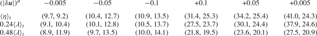
Similarly to  ${\varPi }_{\bar {S}}^{a} - \mathcal {D}^a$, the two p.d.f.s of
  ${\varPi }_{\bar {S}}^a - (\mathcal {D}_{r,\nu }^a-\mathcal {\epsilon }^a)$ in figure 5(b,d, f) which are conditional on the 5 % and 0.5 % highest
  $(\vert \delta \boldsymbol {u}\vert ^2 )^a$ (blue and green curves) have exponential tails which depend on
  $r_d$ in a similar way. Unlike
  ${\varPi }_{\bar {S}}^{a} - \mathcal {D}^a$, however, the p.d.f. of
  ${\varPi }_{\bar {S}}^a - (\mathcal {D}_{r,\nu }^a-\mathcal {\epsilon }^a)$ conditional on the 5 % lowest
  $(\vert \delta \boldsymbol {u}\vert ^2 )^a$ (red curves in figure 5b,d, f) has an exponential tail on its negative side but a stretched exponential tail on its positive side. Whilst the exponential tail on the negative side does not get wider and varies rather weakly with decreasing
  $r_d$ (similarly to the p.d.f.s that are conditional to the 5 % and 0.5 % highest
  $(\vert \delta \boldsymbol {u}\vert ^2 )^a$), the stretched exponential side widens quite appreciably as
  $r_d$ decreases from
  $0.5\langle \lambda \rangle _t$ to
  $\langle \eta \rangle _t$. In low
  $(\vert \delta \boldsymbol {u}\vert ^2 )^a$ regions, the intermittency in the fluctuations of
  ${\varPi }_{\bar {S}}^a - (\mathcal {D}_{r,\nu }^a-\mathcal {\epsilon }^a)$ is therefore much more present and intense with positive rather than negative values of
  ${\varPi }_{\bar {S}}^a - (\mathcal {D}_{r,\nu }^a-\mathcal {\epsilon }^a)$: there are disproportionately many events in such regions with particularly large positive deviations from
  ${\varPi }_{\bar {S}}^a - (\mathcal {D}_{r,\nu }^a-\mathcal {\epsilon }^a) \approx 0$.
As already mentioned, however, even the most likely value of  ${\varPi }_{\bar {S}}^a - (\mathcal {D}_{r,\nu }^a-\mathcal {\epsilon }^a)$ is in fact not zero; when conditioning on the 5 % lowest
  $(\vert \delta \boldsymbol {u}\vert ^2 )^a$ it is positive and when conditioning on the 5 % or 0.5 % highest
  $(\vert \delta \boldsymbol {u}\vert ^2 )^a$ it is negative. As we report in table 1, it is not even particularly likely to find
  ${\varPi }_{\bar {S}}^a \approx (\mathcal {D}_{r,\nu }^a-\mathcal {\epsilon }^a)$. In fact, it is significantly less likely than finding
  ${\varPi }_{\bar {S}}^{a} \approx \mathcal {D}^a$. The probability of finding
  $\tfrac {2}{3}(\mathcal {D}_{r,\nu }^a-\mathcal {\epsilon }^a) < {\varPi }_{\bar {S}}^a < \tfrac {4}{3}(\mathcal {D}_{r,\nu }^a-\mathcal {\epsilon }^a)$ ranges from 9.2 % to 25.4 % whereas the probability of finding
  $\tfrac {2}{3} \mathcal {D}^a < {\varPi }_{\bar {S}}^a <\tfrac {4}{3}\mathcal {D}^a$ ranges from 8.9 % to 41.0 % (table 1). Unlike the latter which increases as we condition on progressively higher
  $(\vert \delta \boldsymbol {u}\vert ^2 )^a$, the probability of finding
  $\tfrac {2}{3}(\mathcal {D}_{r,\nu }^a-\mathcal {\epsilon }^a) < {\varPi }_{\bar {S}}^a < \tfrac {4}{3}(\mathcal {D}_{r,\nu }^a-\mathcal {\epsilon }^a)$ levels off (see table 1). When we condition on increasing values of
  $(\vert \delta \boldsymbol {u}\vert ^2 )^a$ it becomes increasingly difficult to neglect the viscous diffusion in physical space as already noted in the paragraph before (4.1).
We have therefore reached the conclusion that (2.4) is in no way representative of what actually happens at dissipative scales between  $\langle \eta \rangle _t$ and
  $0.5 \langle \lambda \rangle _t$ where (2.4) holds. The local balance
  ${\varPi }_{\bar {S}}^a \approx (\mathcal {D}_{r,\nu }^a-\mathcal {\epsilon }^a)$ is spatiotemporally rather rare. It is only slightly less rare than the local balance
  ${\varPi }_{\bar {S}}^{a} \approx \mathcal {D}^a$ at the lower to moderate levels of
  $(\vert \delta \boldsymbol {u}\vert ^2 )^a$ but significantly rarer than the local balance
  ${\varPi }_{\bar {S}}^{a} \approx \mathcal {D}^a$ at the higher levels of
  $(\vert \delta \boldsymbol {u}\vert ^2 )^a$. It becomes increasingly unlikely for the viscous diffusion in physical space
  $\mathcal {D}_{x,\nu }^a$ to be negligible as
  $(\vert \delta \boldsymbol {u}\vert ^2 )^a$ increases. However, in reaching this conclusion we also found that the probability of finding
  ${\varPi }_{\bar {S}}^{a} \approx \mathcal {D}^a$ is not overwhelming either, and that the p.d.f. of
  ${\varPi }_{\bar {S}}^a - (\mathcal {D}_{r,\nu }^a-\mathcal {\epsilon }^a)$ conditional on the 5 % lowest
  $(\vert \delta \boldsymbol {u}\vert ^2 )^a$ is overwhelmingly weighted towards positive values of
  ${\varPi }_{\bar {S}}^a - (\mathcal {D}_{r,\nu }^a-\mathcal {\epsilon }^a)$. We now address these two remaining issues starting from the second one.
4.2. Correlations
In figure 6(a,b) we report two scatter plots of  $\mathcal {D}_{r,\nu }^a-\mathcal {\epsilon }^a$ and
  ${\varPi }_{\bar {S}}^a$ at
  $r_d = \langle \eta \rangle _t$, one (figure 6a) conditioned on the
  $5\,\%$ lowest values of
  $(\vert \delta \boldsymbol {u}\vert ^2 )^a$ for
  $r_d = \langle \eta \rangle _t$ and the other (figure 6b) conditioned on the
  $5\,\%$ highest values of
  $(\vert \delta \boldsymbol {u}\vert ^2 )^a$ for
  $r_d = \langle \eta \rangle _t$. The black dotted line in both scatter plots is the line where
  ${\varPi }_{\bar {S}}^a = \mathcal {D}_{r,\nu }^a-\mathcal {\epsilon }^a$. Whilst it is very rare to find positive values of
  $\mathcal {D}_{r,\nu }^a-\mathcal {\epsilon }^a$ in both scatter plots (the probability of finding
  $\mathcal {D}_{r,\nu }^a >0$ is in fact only 1.2 % for
  $r_{d} = \langle \eta \rangle _t$), the two scatter plots are otherwise very different. For the
  $5\,\%$ smallest values of
  $(\vert \delta \boldsymbol {u}\vert ^2 )^a$, the scatter plot is approximately symmetric with respect to
  ${\varPi }_{\bar {S}}^a = 0$, i.e. it looks approximately the same on the positive and negative sides of
  ${\varPi }_{\bar {S}}^a$. Given that
  $\mathcal {D}_{r,\nu }^a-\mathcal {\epsilon }^a$ is overwhelmingly negative,
  ${\varPi }_{\bar {S}}^a - (\mathcal {D}_{r,\nu }^a-\mathcal {\epsilon }^{a})$ is overwhelmingly positive when
  ${\varPi }_{\bar {S}}^a$ is positive which accounts for approximately half of all cases given the approximate symmetry of the scatter plot in figure 6(a). The other approximate half of all cases corresponds to negative values of
  ${\varPi }_{\bar {S}}^a$ in which case the scatter plot in figure 6(a) suggests that
  $\mathcal {D}_{r,\nu }^a-\mathcal {\epsilon }^a < {\varPi }_{\bar {S}}^a < 0$ happens more often than
  ${\varPi }_{\bar {S}}^a < \mathcal {D}_{r,\nu }^a-\mathcal {\epsilon }^a < 0$, thereby also favouring positive values of
  ${\varPi }_{\bar {S}}^a - (\mathcal {D}_{r,\nu }^a-\mathcal {\epsilon }^{a})$ though not as much as when
  ${\varPi }_{\bar {S}}^a$ is positive. All in all, from the scatter plot in figure 6(a) one can see why the p.d.f.s of
  ${\varPi }_{\bar {S}}^a - (\mathcal {D}_{r,\nu }^a-\mathcal {\epsilon }^{a})$ conditioned on the
  $5\,\%$ lowest values of
  $(\vert \delta \boldsymbol {u}\vert ^2 )^a$ (red curves in figure 5b,d, f) are so much skewed towards positive values.
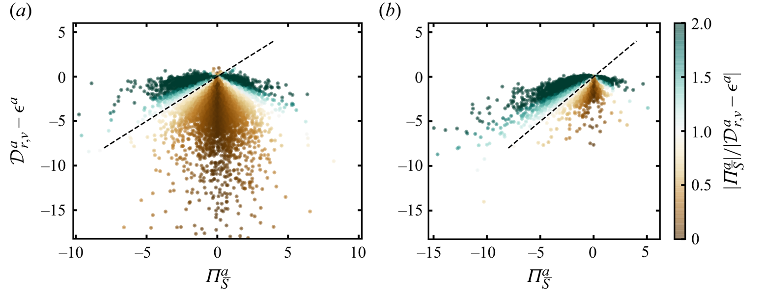
Figure 6. (a) Scatter plot of  $\mathcal {D}_{r,\nu }^a-\mathcal {\epsilon }^a$ and
  ${\varPi }_{\bar {S}}^a$ at
  $r_d = \langle \eta \rangle _t$ conditioned on the
  $5\,\%$ least energetic events (referred to as LE in figure 5). (b) Scatter plot of
  $\mathcal {D}_{r,\nu }^a-\mathcal {\epsilon }^a$ and
  ${\varPi }_{\bar {S}}^a$ at
  $r_d = \langle \eta \rangle _t$ conditioned on the
  $5\,\%$ most energetic events (referred to as HE in figure 5). The black dotted lines show
  ${\varPi }_{\bar {S}}^a=\mathcal {D}_{r,\nu }^a-\mathcal {\epsilon }^a$ and the data points are coloured with the ratio
  $\vert {\varPi }_{\bar {S}}^a\vert /\vert \mathcal {D}_{r,\nu }^a-\mathcal {\epsilon }^a\vert$;
  $\mathcal {D}_{r,\nu }^a-\mathcal {\epsilon }^a$ and
  ${\varPi }_{\bar {S}}^a$ are normalised with the standard deviation of
  ${\varPi }_{\bar {S}}^a$ conditioned on (a) LE events and (b) HE events.
The situation is fundamentally different when we condition on the  $5\,\%$ highest values of
  $(\vert \delta \boldsymbol {u}\vert ^2 )^a$ as the scatter plot of
  $\mathcal {D}_{r,\nu }^a-\mathcal {\epsilon }^a$ and
  ${\varPi }_{\bar {S}}^a$ is no longer symmetric with respect to
  ${\varPi }_{\bar {S}}^a = 0$, see figure 6(b): in fact it is very much skewed towards negative values of
  ${\varPi }_{\bar {S}}^a$. It is therefore impossible to argue that
  ${\varPi }_{\bar {S}}^a - (\mathcal {D}_{r,\nu }^a-\mathcal {\epsilon }^{a})$ is more often positive than negative in this case, and the p.d.f.s of
  ${\varPi }_{\bar {S}}^a - (\mathcal {D}_{r,\nu }^a-\mathcal {\epsilon }^{a})$ conditioned on the
  $5\,\%$ highest values of
  $(\vert \delta \boldsymbol {u}\vert ^2 )^a$ are indeed symmetric around their maximum at zero (see blue curve in figure 5b,d, f). Appendix C shows that the conditional scatter plots in figure 6(a,b) are similar across dissipative scales from
  $r_d \approx \langle \eta \rangle _t$ to
  $r_d \approx 0.5 \langle \lambda \rangle _t$ with the scatter plots being symmetric with respect to
  ${\varPi }_{\bar {S}}^a = 0$ when we condition on low
  $(\vert \delta \boldsymbol {u}\vert ^2 )^a$ values and skewed towards negative values of
  ${\varPi }_{\bar {S}}^a$ when we condition on high
  $(\vert \delta \boldsymbol {u}\vert ^2 )^a$ values.
We now address the last remaining question: given that  ${\varPi }_{\bar {S}}^a - (\mathcal {D}_{r,\nu }^a-\mathcal {\epsilon }^{a})$ is not typically zero even if on average it is, and given that
  ${\varPi }_{\bar {S}}^{a} -\mathcal {D}^a$ is also not so often zero except at the very smallest scales and the regions of highest
  $(\vert \delta \boldsymbol {u}\vert ^2 )^a$, is there a typical energy transfer balance at small dissipative length scales? To shed some light on this question we return to the general solenoidal energy balance (3.1) and plot in figure 7(a) standard deviations of various terms in this equation conditioned on various ranges of
  $(\vert \delta \boldsymbol {u}\vert ^2 )^a$ values. We consider the same 20 ranges of
  $(\vert \delta \boldsymbol {u}\vert ^2 )^a$ values that we considered for figure 4 (see this section's first paragraph), and in the horizontal axes of the two plots in figure 7 we mark each one of these ranges by its average
  $(\vert \delta \boldsymbol {u}\vert ^2 )^a$ value normalised by
  $(\langle \vert \delta \boldsymbol {u}\vert ^2 \rangle ^a$. We do this for
  $r_d = \langle \eta \rangle _t$ in figure 7 and in Appendix C we complete the picture with similar results for some other values of
  $r_d$ in the dissipative range between
  $\langle \eta \rangle _t$ and
  $0.5\langle \lambda \rangle _t$.
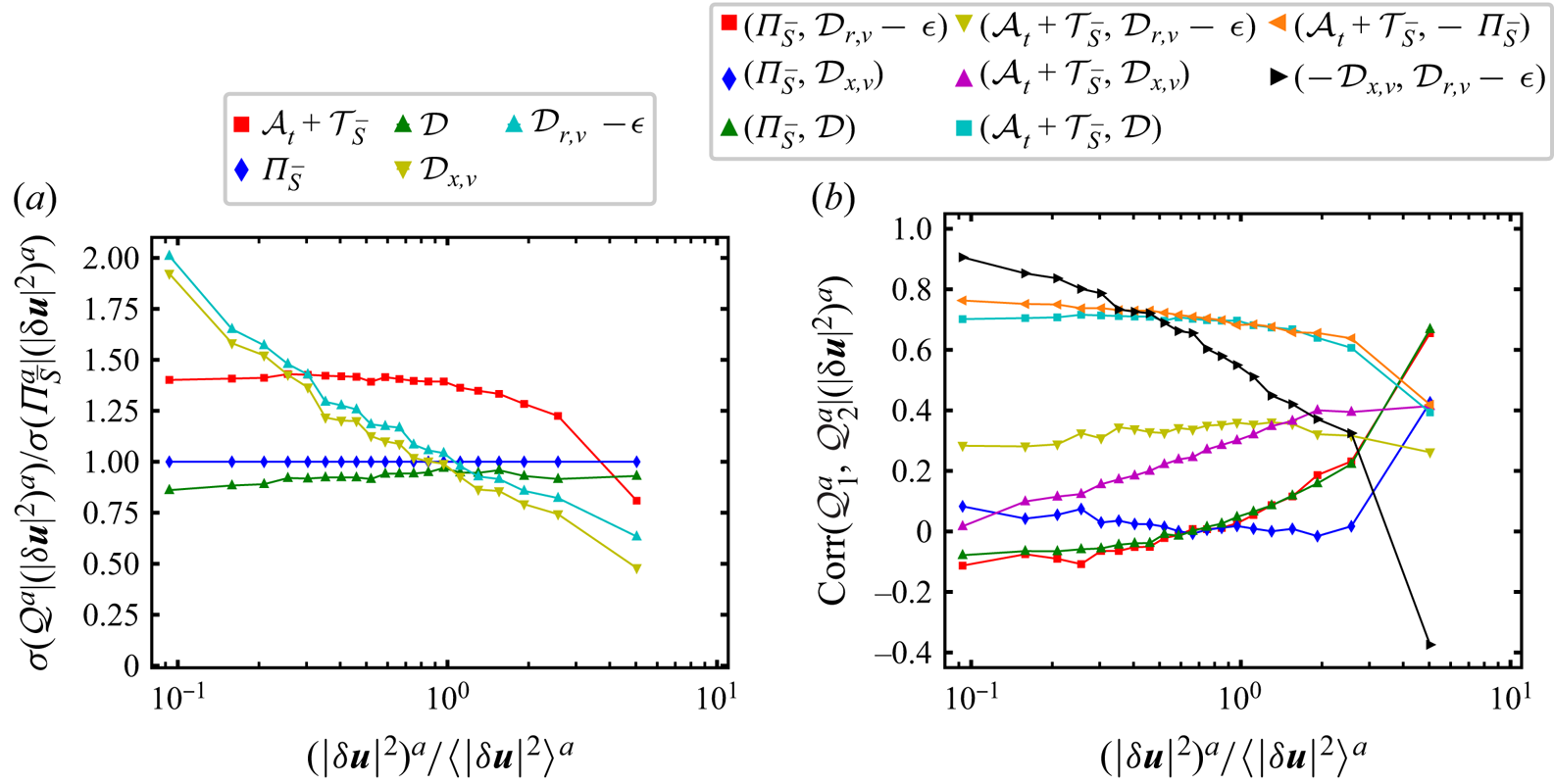
Figure 7. (a) Conditional standard deviations of various surface-averaged KHMH terms  $\mathcal {Q}^{a}$ for
  $r_{d} = \langle \eta \rangle _t$ and (b) conditional Pearson correlation coefficients of pairs of surface-averaged KHMH terms
  $\mathcal {Q}_{1}^{a}$ and
  $\mathcal {Q}_{2}^{a}$ for
  $r_{d} = \langle \eta \rangle _t$. These standard deviations and correlation coefficients are calculated from spatiotemporal statistics conditioned on various ranges of
  $(\vert \delta \boldsymbol {u}\vert ^2 )^a$ at
  $r_d = \langle \eta \rangle _t$. The conditioning is identical to that in figure 4: we consider 20 ranges of
  $(\vert \delta \boldsymbol {u}\vert ^2 )^a$ values and the horizontal axes display the average
  $(\vert \delta \boldsymbol {u}\vert ^2 )^a$ values within each
  $(\vert \delta \boldsymbol {u}\vert ^2 )^a$ range normalised by the spatiotemporally averaged small-scale energy
  $\langle |\delta \boldsymbol {u}|^2 \rangle ^a$. Increasing values of
  $(\vert \delta \boldsymbol {u}\vert ^2 )^a$ are therefore from left to right on the horizontal axes.
Figure 7(a) shows that the standard deviations of  ${\varPi }_{\bar {S}}^{a}$ and
  $\mathcal {D}^a$ are quite close to each other for all
  $(\vert \delta \boldsymbol {u}\vert ^2 )^a$ levels but that the standard deviation of
  ${\varPi }_{\bar {S}}^{a}$ is nevertheless consistently higher than that of
  $\mathcal {D}^a$. The only other term in
  $\mathcal {A}_t^a+\mathcal {T}_{\bar {S}}^a + {\varPi }_{\bar {S}}^{a} = \mathcal {D}^a$ is
  $\mathcal {A}_t^a+\mathcal {T}_{\bar {S}}^a$, and the fluctuations of
  $\mathcal {A}_t^a+\mathcal {T}_{\bar {S}}^a$ are never negligible, in fact they are significantly more intense than those of
  ${\varPi }_{\bar {S}}^{a}$ and
  $\mathcal {D}^a$ at all
  $(\vert \delta \boldsymbol {u}\vert ^2 )^a$ levels except the highest
  $(\vert \delta \boldsymbol {u}\vert ^2 )^a$ considered here. Except perhaps at specific spatiotemporal instances, it is in general not possible to neglect what is effectively the Lagrangian transport term
  $\mathcal {A}_t^a+\mathcal {T}_{\bar {S}}^a$ (see Larssen & Vassilicos Reference Larssen and Vassilicos2023) at these dissipative length scales.
Figure 7(a) also shows that the standard deviations of  ${\varPi }_{\bar {S}}^{a}$ and
  $\mathcal {D}_{r,\nu }^a-\mathcal {\epsilon }^a$ differ significantly at all
  $(\vert \delta \boldsymbol {u}\vert ^2 )^a$ levels except intermediate ones. Furthermore, the standard deviations of
  $\mathcal {D}_{r,\nu }^a-\mathcal {\epsilon }^a$ and
  $\mathcal {D}_{x,\nu }^a$ are very close to each other, the standard deviation of
  $\mathcal {D}_{r,\nu }^a-\mathcal {\epsilon }^a$ being in fact slightly larger than the standard deviation of
  $\mathcal {D}_{x,\nu }^a$ for all
  $(\vert \delta \boldsymbol {u}\vert ^2 )^a$ levels. Both standard deviations decrease with increasing
  $(\vert \delta \boldsymbol {u}\vert ^2 )^a$ whilst the standard deviation of their sum
  $\mathcal {D}^a$ remains approximately constant by comparison. This suggests an anticorrelation between
  $\mathcal {D}_{r,\nu }^a-\mathcal {\epsilon }^a$ and
  $\mathcal {D}_{x,\nu }^a$ where/when
  $(\vert \delta \boldsymbol {u}\vert ^2 )^a$ is low and a synergy/correlation between these two terms where/when
  $(\vert \delta \boldsymbol {u}\vert ^2 )^a$ is high. The conditional correlation coefficient between
  $-\mathcal {D}_{x,\nu }^a$ and
  $\mathcal {D}_{r,\nu }^a-\mathcal {\epsilon }^a$ in figure 7(b) confirms this suggestion. It monotonically decreases with increasing
  $(\vert \delta \boldsymbol {u}\vert ^2 )^a$ from
  $0.9$ at the lowest
  $(\vert \delta \boldsymbol {u}\vert ^2 )^a$ level to nearly
  $-0.4$ at the highest.
Conditional correlations of various other pairs of terms appearing in (3.1) are also plotted in figure 7(b). At the low to moderate  $(\vert \delta \boldsymbol {u}\vert ^2 )^a$ levels there is a correlation of approximately 0.7 between
  $\mathcal {A}_t^a+\mathcal {T}_{\bar {S}}^a$ and
  $-{\varPi }_{\bar {S}}^a$ and also between
  $\mathcal {A}_t^a+\mathcal {T}_{\bar {S}}^a$ and
  $\mathcal {D}^a$. However, there is effectively no correlation at these
  $(\vert \delta \boldsymbol {u}\vert ^2 )^a$ levels between
  ${\varPi }_{\bar {S}}^{a}$ and any of the diffusion/dissipation terms
  $\mathcal {D}^a$,
  $\mathcal {D}_{x,\nu }^a$ and
  $\mathcal {D}_{r,\nu }^a-\mathcal {\epsilon }^a$. The significant correlations which exist between
  $\mathcal {A}_t^a+\mathcal {T}_{\bar {S}}^a$ and
  $-{\varPi }_{\bar {S}}^a$ on the one hand and between
  $\mathcal {A}_t^a+\mathcal {T}_{\bar {S}}^a$ and
  $\mathcal {D}^a$ on the other must therefore arise from different spatiotemporal instances given the absence of correlation between
  ${\varPi }_{\bar {S}}^{a}$ and
  $\mathcal {D}^a$. The picture suggested by
  $\mathcal {A}_t^a+\mathcal {T}_{\bar {S}}^a + {\varPi }_{\bar {S}}^{a} = \mathcal {D}^a$ and by these presences and absences of correlations conditioned on low to moderate
  $(\vert \delta \boldsymbol {u}\vert ^2 )^a$ levels is as follows: as turbulence energy at scale
  $r_d = \langle \eta \rangle _t$ is transported along a Lagrangian path, part of it may at one time be transferred to another scale and part of it may at another time be dissipated and diffused by viscosity, but very rarely will both significantly happen at the same time. There is indeed little spatiotemporal coincidence between interscale transfer rate and diffusion/dissipation at these
  $(\vert \delta \boldsymbol {u}\vert ^2 )^a$ levels. To complete the picture, viscous diffusion in space acts against viscous diffusion/dissipation
  $\mathcal {D}_{r,\nu }^a-\mathcal {\epsilon }^a$ at low to moderate
  $(\vert \delta \boldsymbol {u}\vert ^2 )^a$ levels: whilst
  $\mathcal {D}_{r,\nu }^a-\mathcal {\epsilon }^a$ most typically removes energy,
  $\mathcal {D}_{x,\nu }^a$ counteracts by adding energy at that scale from neighbouring physical space. As shown in Appendix C this picture is essentially true for all scales
  $r_d$ between
  $\langle \eta \rangle _t$ and
  $0.5\langle \lambda \rangle _t$. With increasing
  $r_d$ the standard deviations of viscous effects
  $\mathcal {D}^a$ decrease relative to those of
  ${\varPi }_{\bar {S}}$ and
  $\mathcal {A}_t^a+\mathcal {T}_{\bar {S}}^a$. This leads to weaker correlations between
  $\mathcal {D}^a$ and
  ${\varPi }_{\bar {S}}^a$ and stronger correlations between
  $\mathcal {A}_t^a+\mathcal {T}_{\bar {S}}^a$ and
  $-{\varPi }_{\bar {S}}^a$.
The picture (described now for  $r_{d}=\langle \eta \rangle _t$ but confirmed in Appendix C for other
  $r_{d} < 0.5\langle \lambda \rangle _t$) changes dramatically as we reach the 5 % highest
  $(\vert \delta \boldsymbol {u}\vert ^2 )^a$ levels, i.e. levels between approximately 30 to 60 times
  $(\langle \vert \delta \boldsymbol {u}\vert ^2 \rangle ^a$. Firstly, at such high local kinetic energy levels,
  $\mathcal {D}_{r,\nu }^a-\mathcal {\epsilon }^a$ and
  $\mathcal {D}_{x,\nu }^a$ acquire some significant tendency to act together (correlation coefficient of approximately
  $0.4$) to remove kinetic energy from scale
  $r_d = \langle \eta \rangle _t$. This is a remarkable reversal in the role played by viscous diffusion in physical space. Secondly, the correlations of
  $\mathcal {A}_t^a+\mathcal {T}_{\bar {S}}^a$ with
  $-{\varPi }_{\bar {S}}^a$ and with
  $\mathcal {D}^a$ drop but remain significant (correlation coefficients of approximately
  $0.4$) whilst
  ${\varPi }_{\bar {S}}^a$ acquires substantial correlation with the diffusion/dissipation terms: its correlation coefficients with
  $\mathcal {D}^a$ and with
  $\mathcal {D}_{r,\nu }^a - \mathcal {\epsilon }^a$ rise to approximately 0.7, and its correlation coefficient with
  $\mathcal {D}_{x,\nu }^a$ rises too but not so much (it reaches approximately
  $0.4$). At these particularly high
  $(\vert \delta \boldsymbol {u}\vert ^2 )^a$ levels and very small scales
  $\langle \eta \rangle _t$, the strongest correlation is therefore the one between
  ${\varPi }_{\bar {S}}^a$ and
  $\mathcal {D}^a$ but it is not so strong that we may neglect the Lagrangian transport term
  $\mathcal {A}_t^a+\mathcal {T}_{\bar {S}}^a$, i.e. the remaining term in the full balance
  $\mathcal {A}_t^a+\mathcal {T}_{\bar {S}}^a + {\varPi }_{\bar {S}}^a = \mathcal {D}^a$, which is also significantly correlated with both
  $-{\varPi }_{\bar {S}}^a$ and
  $\mathcal {D}^a$. We chose to focus on the correlation between
  ${\varPi }_{\bar {S}}^a$ and
  $\mathcal {D}^a$ rather than between
  ${\varPi }_{\bar {S}}^a$ and
  $\mathcal {D}_{r,\nu }^a-\mathcal {\epsilon }^a$ even though they have the same correlation coefficients because we have seen that, unlike
  ${\varPi }_{\bar {S}}^a$ and
  $\mathcal {D}_{r,\nu }^a-\mathcal {\epsilon }^a$,
  ${\varPi }_{\bar {S}}^a$ and
  $\mathcal {D}^a$ have an increasing statistical tendency to get close to each other with increasing
  $(\vert \delta \boldsymbol {u}\vert ^2 )^a$ levels and decreasing length scale (see figure 4, table 1 and figure 11). However, this does not happen without some correlation with Lagrangian transport.
Appendix C and figure 11 show that as we consider larger scales, the viscous terms become gradually less important locally and the dynamics tend to the approximate local (in space–time) balance reported in Larssen & Vassilicos (Reference Larssen and Vassilicos2023),  $\mathcal {A}_t^{a}+\mathcal {T}_{\bar {S}}^{a} \approx - {\varPi }_{\bar {S}}^{a'}$ (see also the unconditional correlation coefficients in figure 2d). At
  $r_d=0.48 \langle \eta \rangle _t$, across various
  $(\vert \delta \boldsymbol {u}\vert ^2 )^a$-levels,
  $\mathcal {A}_t^{a}+\mathcal {T}_{\bar {S}}^{a}$ and
  ${\varPi }_{\bar {S}}^{a}$ have correlations approximately equalling
  $0.90$ and the standard deviations of
  ${\varPi }_{\bar {S}}^{a}$ are typically twice as large as those of
  $\mathcal {D}^a$.
5. Summary of conclusions
In statistically stationary homogeneous/periodic turbulence the average relation  $\langle {\varPi }_{\bar {S}}^{a} \rangle \approx \langle \mathcal {D}_{r,\nu }^{a} \rangle - \langle \mathcal {\epsilon }^{a}\rangle$ holds in the dissipation/diffusion-dominated range
  $r_{d} < 0.5 \langle \lambda \rangle _t$, yet it does not represent reality locally in space and time. Events where
  ${\varPi }_{\bar {S}}^{a} \approx \mathcal {D}_{r,\nu }^{a} - \mathcal {\epsilon }^{a}$ can of course be found but they are few and far between. What actually happens at these small length scales cannot be described without
  $\mathcal {A}_t^a+\mathcal {T}_{\bar {S}}^a$ even though the fluctuation amplitudes of this Lagrangian transport term (which vanishes on average) decrease towards zero with decreasing
  $r_d$ in the dissipation/diffusion-dominated range
  $r_{d} < 0.5 \langle \lambda \rangle _t$.
In most of the flow for most of the time the levels of  $(\vert \delta \boldsymbol {u}\vert ^2 )^a$ at these length scales are low to moderate and one finds significant correlations between
  $\mathcal {A}_t^a+\mathcal {T}_{\bar {S}}^a$ and
  ${\varPi }_{\bar {S}}^{a}$ on the one hand and between
  $\mathcal {A}_t^a+\mathcal {T}_{\bar {S}}^a$ and
  $\mathcal {D}^{a}$ on the other. There are interscale transfer events happening along some parts of Lagrangian path and diffusion/dissipation events happening along some other parts of the Lagrangian path, but rarely do they happen together. Also, viscous diffusion in space is typically positive and counteracts the energy reducing action of
  $\mathcal {D}^a_{r,\nu }-\mathcal {\epsilon }^a$ which is typically negative.
As we focus on the highest levels of  $(\vert \delta \boldsymbol {u}\vert ^2 )^a$ at these length scales the picture changes quite drastically but
  $\mathcal {A}_t^a+\mathcal {T}_{\bar {S}}^a$ maintains a presence even if weakened. The highest correlation is now between
  ${\varPi }_{\bar {S}}^{a}$ and
  $\mathcal {D}^{a}$. Even though this correlation is similar to that of
  ${\varPi }_{\bar {S}}^{a}$ and
  $\mathcal {D}^a_{r,\nu }-\mathcal {\epsilon }^a$, we have seen that there is much more of a tendency for
  ${\varPi }_{\bar {S}}^{a}$ and
  $\mathcal {D}^{a}$ to get close to each other than
  ${\varPi }_{\bar {S}}^{a}$ and
  $\mathcal {D}^a_{r,\nu }-\mathcal {\epsilon }^a$. This does not happen perfectly though given that
  $\mathcal {A}_t^a+\mathcal {T}_{\bar {S}}^a$ retains some correlation with both
  $-{\varPi }_{\bar {S}}^{a}$ and
  $\mathcal {D}^a$, which means that all terms in
  $\mathcal {A}_t^a+\mathcal {T}_{\bar {S}}^a + {\varPi }_{\bar {S}}^{a} = \mathcal {D}^a$ can momentarily follow each other simultaneously at these very high
  $(\vert \delta \boldsymbol {u}\vert ^2 )^a$ levels.
It is important to stress the role of viscous diffusion in physical space which cannot be typically neglected from the balance of  ${\varPi }_{\bar {S}}^{a}$ at the very high
  $(\vert \delta \boldsymbol {u}\vert ^2 )^a$ regions where there is of course high local inhomogeneity. Furthermore, in these regions the viscous diffusion in physical space does not resist any longer but in fact acquires a tendency to cooperate with
  $\mathcal {D}^a_{r,\nu }-\mathcal {\epsilon }^a$ and enhance energy reduction.
An ingredient that is sometimes used for the derivation of local viscous length scales is the assumption of a local balance between a local turnover time and a local viscous diffusion time (Paladin & Vulpiani Reference Paladin and Vulpiani1987; Frisch & Vergassola Reference Frisch and Vergassola1991; Dubrulle Reference Dubrulle2019). This typically amounts to a local balance between interscale transfer rate and viscous diffusion in scale space/dissipation, i.e.  ${\varPi }_{\bar {S}}^{a} \approx \mathcal {D}_{r,\nu }^{a} - \mathcal {\epsilon }^{a}$. The present study might offer a more complete view of the types of local and instantaneous balances which might be used to obtain local viscous length scales.
Acknowledgements
We thank Professor S. Goto for allowing us to use his parallelised pseudospectral DNS code for periodic turbulence.
Funding
H.S.L. and J.C.V. acknowledge support from EPSRC award number EP/L016230/1. Furthermore, J.C.V. acknowledges the Chair of Excellence CoPreFlo funded by I-SITE-ULNE (grant no. R-TALENT-19-001-VASSILICOS), MEL (grant no. CONVENTION-219-ESR-06) and Region Hauts de France (grant no. 20003862); and also funding by the European Union (ERC Advanced Grant NoStaHo, project number 101054117). Views and opinions expressed are, however, those of the author(s) only and do not necessarily reflect those of the European Union or the European Research Council. Neither the European Union nor the granting authority can be held responsible for them.
Declaration of interests
The authors report no conflict of interest.
Appendix A. The KHMH equation and associated Helmholtz decomposition
The KHMH equation is derived directly from the incompressible Navier–Stokes equations at locations  $\boldsymbol {x}^{+}$ and
  $\boldsymbol {x}^{-}$ and it governs the evolution of the velocity difference squared,
  $\vert \delta \boldsymbol {u} \vert ^2$ (Hill Reference Hill2002). It is written in terms of the centroid
  $\boldsymbol {x} = (\boldsymbol {x}^{+} + \boldsymbol {x}^{-})/2$ and separation
  $\boldsymbol {r}= \boldsymbol {x}^{+} -\boldsymbol {x}^{-}$ vectors and differences of scalar and vector fields. The symbol
  $\delta$ preceding a scalar or vector field
  $\phi$ denotes
  $\delta \phi = \phi ^{+}-\phi ^{-}$ where
  $\phi ^{+}=\phi (\boldsymbol {x}+\boldsymbol {r}/2,t)$ and
  $\phi ^{-}=\phi (\boldsymbol {x}-\boldsymbol {r}/2,t)$. With this notation the KHMH equation reads
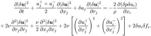 $$\begin{gather} \frac{\partial |\delta \boldsymbol{u}|^2}{\partial t} + \frac{u_j^{+}+u_j^{-}}{2} \frac{\partial |\delta \boldsymbol{u}|^2}{\partial x_j} + \delta u_j \frac{\partial |\delta \boldsymbol{u}|^2}{\partial r_j} ={-} \frac{2}{\rho}\frac{\partial (\delta p \delta u_i)}{\partial x_i} \nonumber\\ +\,2\nu \frac{\partial^2 |\delta \boldsymbol{u}|^2}{\partial r_j \partial r_j}+\frac{\nu}{2}\frac{\partial^2 |\delta \boldsymbol{u}|^2}{\partial x_j \partial x_j}+2\nu \left[ \left(\frac{\partial u_i^{+}}{\partial x_j^{+}}\right)^2+\left(\frac{\partial u_i^{-}}{\partial x_j^{-}}\right)^2 \right] + 2\delta u_i\delta f_i. \end{gather}$$
We associate the KHMH terms with the following physical processes (Yasuda & Vassilicos Reference Yasuda and Vassilicos2018):
 \begin{align} \mathcal{A}_t(\boldsymbol{x},\boldsymbol{r},t) &\equiv \partial/\partial t (|\delta \boldsymbol{u}|^2) \text{ is the local unsteadiness},\text{ or time-derivative},\text{ term}; \end{align}
 \begin{align} \mathcal{T}(\boldsymbol{x},\boldsymbol{r},t) &\equiv \partial/\partial x_k ((u_k^{+}+u_k^{-})|\delta \boldsymbol{u}|^2/2) \text{ is the turbulent transport term}; \end{align}
 \begin{align} {\varPi}(\boldsymbol{x},\boldsymbol{r},t) &\equiv \partial/\partial r_k (\delta u_k |\delta \boldsymbol{u}|^2) \text{ is the interscale energy transfer term}; \end{align}
 \begin{align} \mathcal{T}_p(\boldsymbol{x},\boldsymbol{r},t) &\equiv{-}(2/\rho)\partial/\partial x_k (\delta u_k \delta p) \text{ is the pressure-velocity term}; \end{align}
 \begin{align} \mathcal{D}_{r,\nu}(\boldsymbol{x},\boldsymbol{r},t) &\equiv 2\nu \partial^2/\partial r_k^2(|\delta \boldsymbol{u}|^2) \text{ is the viscous diffusion in }\boldsymbol{r}\text{-space}; \end{align}
 \begin{align} \mathcal{D}_{x,\nu}(\boldsymbol{x},\boldsymbol{r},t) &\equiv \nu \partial^2/\partial x_k^2(|\delta \boldsymbol{u}|^2/2) \text{ is the viscous diffusion in }\boldsymbol{x}\text{-space}; \end{align}
 \begin{align} \mathcal{I}(\boldsymbol{x},\boldsymbol{r},t)&\equiv 2\delta u_k \delta f_k \text{ is the energy input rate}; \end{align}
 \begin{align} \mathcal{\epsilon}^{*}(\boldsymbol{x},\boldsymbol{r},t)&\equiv 2\nu[(\partial u_j^{+}/\partial x_k^{+}))^2+(\partial u_j^{-}/\partial x_k^{-}))^2] \\ &\quad \text{ is two times the sum of the pseudodissipation at }\boldsymbol{x}^{+}\text{ and }\boldsymbol{x}^{-}. \nonumber \end{align}
Larssen & Vassilicos (Reference Larssen and Vassilicos2023) split the KHMH equation (A1) into two new KHMH equations (see (2.1)–(2.2)): one equation arising from the centroid solenoidal  $\delta \boldsymbol {u}$ dynamics and one equation arising from the centroid irrotational
  $\delta \boldsymbol {u}$ dynamics. This Helmholtz decomposition gives rise to four new KHMH terms: the irrotational and solenoidal interspace transport terms
  $\mathcal {T}_{\bar {I}}$ and
  $\mathcal {T}_{\bar {S}}$ and the irrotational and solenoidal interscale transfer terms
  ${\varPi }_{\bar {I}}$ and
  ${\varPi }_{\bar {S}}$.
We calculate these terms in this study in terms of the irrotational KHMH equation and the pressure-velocity term (see § 2), but they can also be calculated explicitly in Fourier space in a periodic domain at a higher computational cost (Larssen & Vassilicos Reference Larssen and Vassilicos2023). The solenoidal and irrotational interscale transfer terms read  ${\varPi }_{\bar {S}}=2\delta \boldsymbol {u} \boldsymbol {\cdot } \boldsymbol {a}_{{\varPi }_{\bar {S}}}$ and
  ${\varPi }_{\bar {I}}=2\delta \boldsymbol {u} \boldsymbol {\cdot } \boldsymbol {a}_{{\varPi }_{\bar {I}}}$ and the solenoidal and irrotational transport terms read
  $\mathcal {T}_{\bar {S}}=2\delta \boldsymbol {u} \boldsymbol {\cdot } \boldsymbol {a}_{\mathcal {T}_{\bar {S}}}$ and
  $\mathcal {T}_{\bar {I}}=2\delta \boldsymbol {u} \boldsymbol {\cdot } \boldsymbol {a}_{\mathcal {T}_{\bar {I}}}$, where
  $\boldsymbol {a}_{{\varPi }}=\delta \boldsymbol {u} \boldsymbol {\cdot } \boldsymbol {\nabla }_{\boldsymbol {r}} \delta \boldsymbol {u}$,
  $\boldsymbol {a}_{\mathcal {T}}=\tfrac {1}{2}(\boldsymbol {u}^{+}+\boldsymbol {u}^{-})\boldsymbol {\cdot } \boldsymbol {\nabla }_{\boldsymbol {x}} \delta \boldsymbol {u}$. Here
  $\boldsymbol {q}_{\bar {S}}(\boldsymbol {x},\boldsymbol {r},t)$ denotes the solenoidal part of a vector field
  $\boldsymbol {q}(\boldsymbol {x},\boldsymbol {r},t)$ and
  $\boldsymbol {q}_{\bar {I}}(\boldsymbol {x},\boldsymbol {r},t)$ denotes the solenoidal part of
  $\boldsymbol {q}(\boldsymbol {x},\boldsymbol {r},t)$. When calculated explicitly in a periodic domain, one calculates the solenoidal and irrotational parts of
  $\boldsymbol {a}_{{\varPi }}$ and
  $\boldsymbol {a}_{\mathcal {T}}$ with the standard Helmholtz decomposition in Fourier space before calculating the KHMH analogue terms by contracting with
  $2\delta \boldsymbol {u}$.
Appendix B. The KHMH numerical integration and residual
In this appendix we detail our KHMH numerical spherical averaging operation and the KHMH residual. Let  $\mathcal {Q}$ denote an arbitrary KHMH term. The spherical averaging operation can be written as
 \begin{align} \mathcal{Q}^a &= \frac{1}{{\rm \pi} r_d^2} \iiint_{\vert \boldsymbol{r} \vert =r_d} \mathcal{Q} \,{\rm d}\boldsymbol{r}, \end{align}
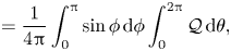 \begin{align} & = \frac{1}{4{\rm \pi}} \int_{0}^{\rm \pi} \sin\phi \,{\rm d} \phi \int_{0}^{2{\rm \pi}} \mathcal{Q} \, {\rm d}\theta, \end{align}
where  $\theta$ and
  $\phi$ denote the polar and azimuthal angles (see figure 8a). We approximate (B2) numerically by repeated one-dimensional quadratures
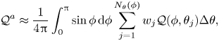 \begin{align} \mathcal{Q}^a &\approx \frac{1}{4{\rm \pi}} \int_{0}^{\rm \pi} \sin \phi \,{\rm d} \phi \sum_{j=1}^{N_\theta(\phi)} w_j \mathcal{Q}(\phi, \theta_j) \Delta \theta, \end{align}
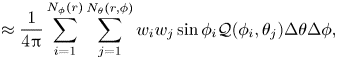 \begin{align} &\approx \frac{1}{4{\rm \pi}} \sum_{i=1}^{N_{\phi}(r)} \sum_{j=1}^{N_\theta(r, \phi)} w_i w_j \sin \phi_i \mathcal{Q}(\phi_i, \theta_j) \Delta \theta \Delta \phi, \end{align}
where  $w_i$ and
  $w_j$ are integration weights,
  $N_{\phi }$ and
  $N_{\theta }$ are the number of grid points in azimuthal and polar directions,
  $\Delta \theta$ and
  $\Delta \phi$ are the spherically equidistant integration spacings and
  $r$ denotes the integration radius in integer grid points. For a given
  $r$ we have
  $N_{\phi }=4r+1$ and
  $N_{\theta }=8r_{\phi }=8r\sin \phi$ available grid points where
  $r_{\phi }$ denotes the radius of the circle at the given
  $\phi$ value (see figure 8b). The grid spacings are given as
  $\Delta \phi = ({{\rm \pi} }/({N_{\phi }(r)-1}))$ and
  $\Delta \theta = ({2{\rm \pi} }/({N_{\theta }(r, \phi )-1}))$. We use Simpson's rule to set the weights
  $w_i$ and
  $w_j$.
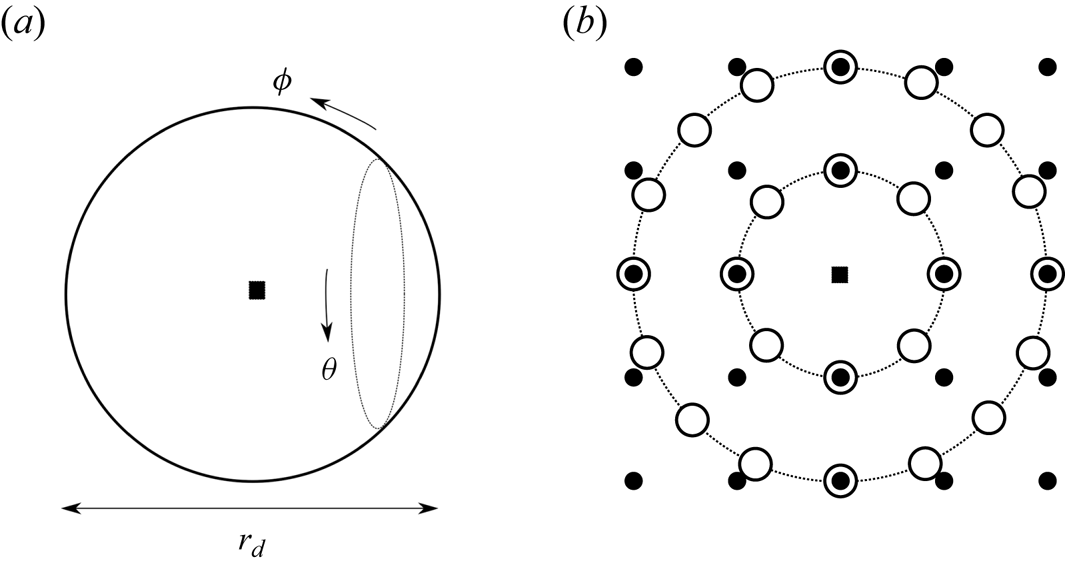
Figure 8. (a) Sketch of the spherical coordinate system and the filled square denotes original. (b) Sketch of the integration and grid points with spherical equidistant integration for  $r=1$ and
  $r=2$. The filled circles are grid points and the open circles are the integration points.
The equidistant approach limits the distance between grid points and integration points (see figure 8b) such that we limit the effect of interpolation errors in the computation of the KHMH terms  $\mathcal {Q}(\phi _i, \theta _j)$ in (B4). This is important at small scales where the grid spacing and the scales of interest are of similar order of magnitude. This contrasts with a Lebedev quadrature approach where interpolation errors from a discrete grid are not considered (Lebedev Reference Lebedev1975). As we do not calculate the entire
  $\mathcal {Q}$ field in
  $\boldsymbol {x}$-space, we cannot use the recent integration method of Iyer et al. (Reference Iyer, Bonaccorso, Biferale and Toschi2017), which spectrally interpolates the field of interest to Lebedev integration points.
The smallest integration sphere we employ is the sphere with  $r=1$ and
  $r_d \approx \langle \eta \rangle _t$. This results in coarse spherical averages
  $\mathcal {Q}^a$ (i.e. 26 integration points). The spherically averaged
  $\mathcal {Q}$ might not be converged in terms of the spherical integration and one should be careful when comparing absolute statistics such as
  $\langle \mathcal {Q}^a\rangle$ at small scales between studies using coarse surface integrations. We get a lower estimate of the integration error at
  $r=1$ by integrating a constant over the sphere with a relative error of
  $3\times 10^{-3}$. In terms of relative magnitudes, the coarseness of the spherical averaging does not invalidate relative statements between KHMH terms
  $\mathcal {Q}_1^a$ and
  $\mathcal {Q}_2^a$ such as
  $\mathcal {Q}_1^a \gg \mathcal {Q}_2^a$. We see from (B4) that the local difference between KHMH terms
  $\mathcal {Q}_1^a$ and
  $\mathcal {Q}_2^a$ can only be considerable if
  $\mathcal {Q}_1 \gg \mathcal {Q}_2$ in an average sense over the considered separations
  $\boldsymbol {r}$.
We can use the solenoidal KHMH equation to assess the accuracy of the computed KHMH terms. We denote the local residual of the solenoidal KHMH equation by  $R$ and its spherical average
  $R^{a}$. We plot in figure 9 the
  $R^{a}$ spatiotemporal averages and standard deviations across scales. This shows that even at small scales the KHMH terms are calculated satisfactorily. The averages and standard deviations of the residual are always an order of magnitude smaller than the average and standard deviation solenoidal interscale transfer term, which is characteristic of the small-scale cascade dynamics.
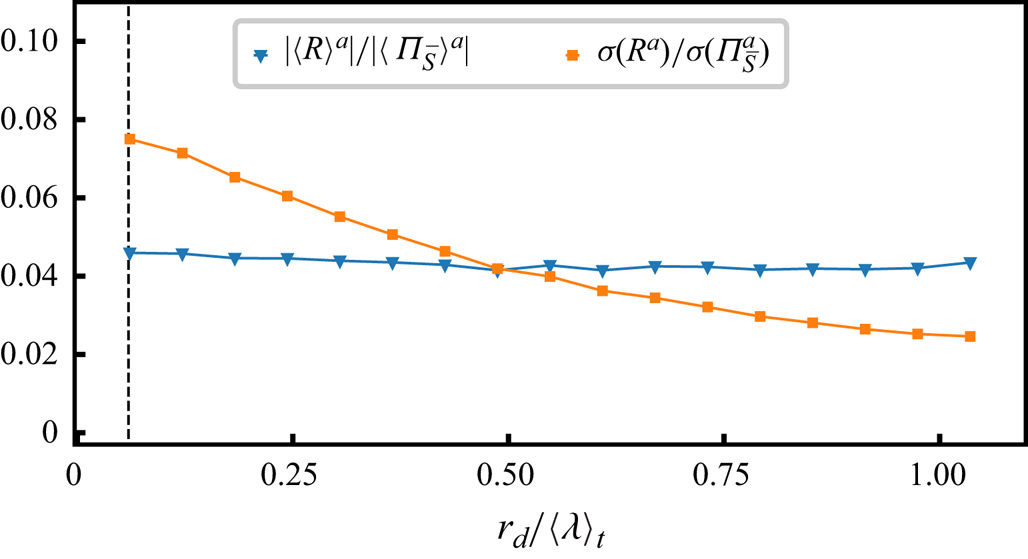
Figure 9. Surface-averaged solenoidal KHMH equation residual  $R^a$ spatiotemporal averages and standard deviations across small scales. The vertical line denotes
  $r_d=\langle \eta \rangle _t$.
Appendix C. Conditional KHMH statistics across scales
The plots in figures 6 and 7 are given for  $r_{d} = \langle \eta \rangle _t$. Here we complement these figures with the same plots in figures 10 and 11 for other values of
  $r_{d}$ between
  $\langle \eta \rangle _t$ and
  $0.5\langle \lambda \rangle _t$ in support of the claim that the conclusions derived from figures 6 and 7 in the paper's main text are valid for the range of dissipative/diffusive length scales between
  $\langle \eta \rangle _t$ and
  $0.5\langle \lambda \rangle _t$.
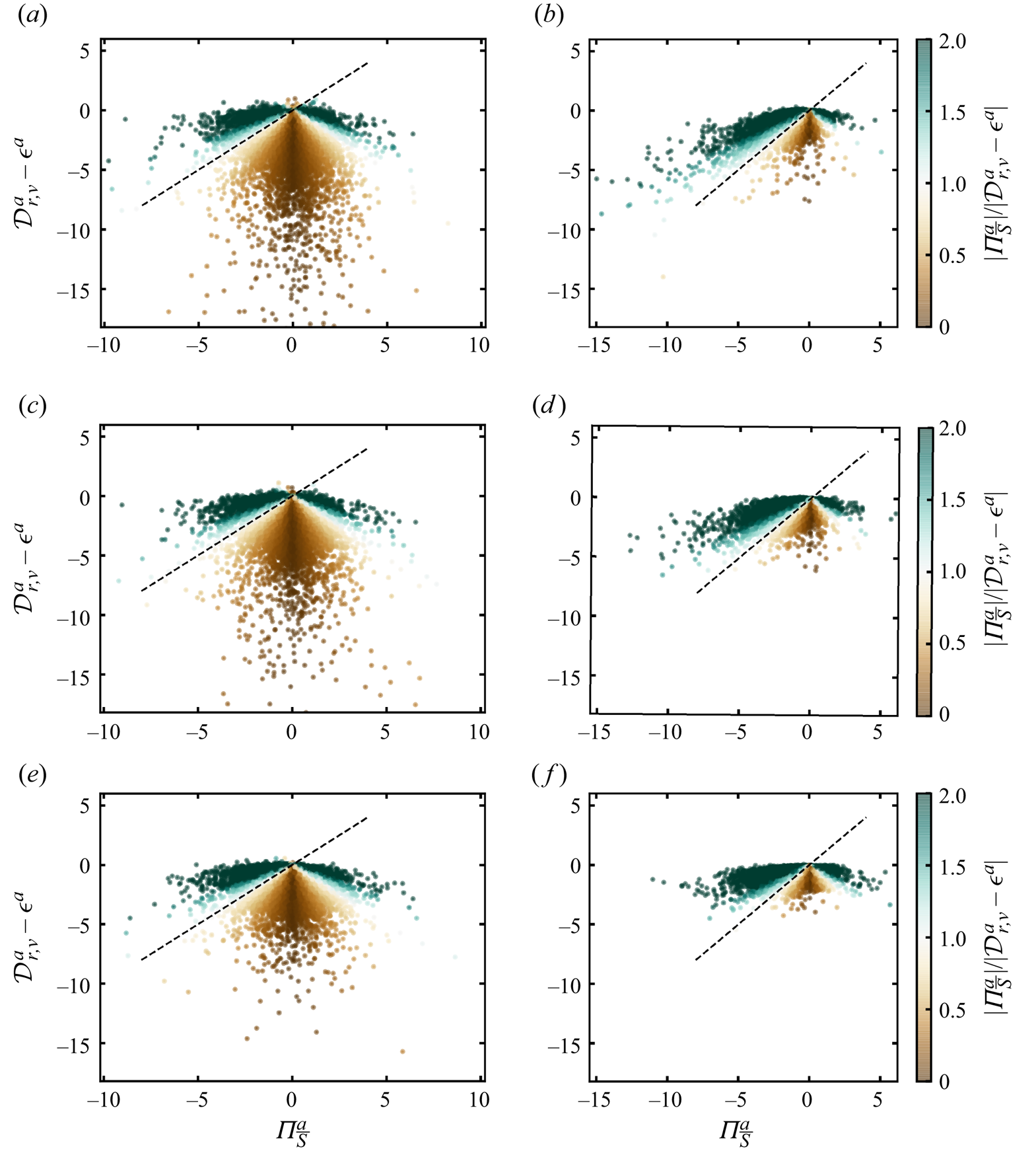
Figure 10. (a,c,e) Scatter plots of  $\mathcal {D}_{r,\nu }^a-\mathcal {\epsilon }^a$ and
  ${\varPi }_{\bar {S}}^a$ at (a)
  $r_d = \langle \eta \rangle _t$, (c)
  $r_d = \langle 0.24 \lambda \rangle _t$ and (e)
  $r_d = \langle 0.48 \lambda \rangle _t$ conditioned on the
  $5\,\%$ least energetic events (referred to as LE in figure 5). (b,d, f) Scatter plots of
  $\mathcal {D}_{r,\nu }^a-\mathcal {\epsilon }^a$ and
  ${\varPi }_{\bar {S}}^a$ at (b)
  $r_d = \langle \eta \rangle _t$, (d)
  $r_d = \langle 0.24 \lambda \rangle _t$ and ( f)
  $r_d = \langle 0.48 \lambda \rangle _t$ conditioned on the
  $5\,\%$ most energetic events (referred to as HE in figure 5). The black dotted lines show
  ${\varPi }_{\bar {S}}^a=\mathcal {D}_{r,\nu }^a-\mathcal {\epsilon }^a$ and the data points are coloured with the ratio
  $\vert {\varPi }_{\bar {S}}^a\vert /\vert \mathcal {D}_{r,\nu }^a-\mathcal {\epsilon }^a\vert$. Here
  $\mathcal {D}_{r,\nu }^a-\mathcal {\epsilon }^a$ and
  ${\varPi }_{\bar {S}}^a$ are normalised with the standard deviation of
  ${\varPi }_{\bar {S}}^a$ conditioned on (a,c,e) LE events and (b,d, f) HE events.
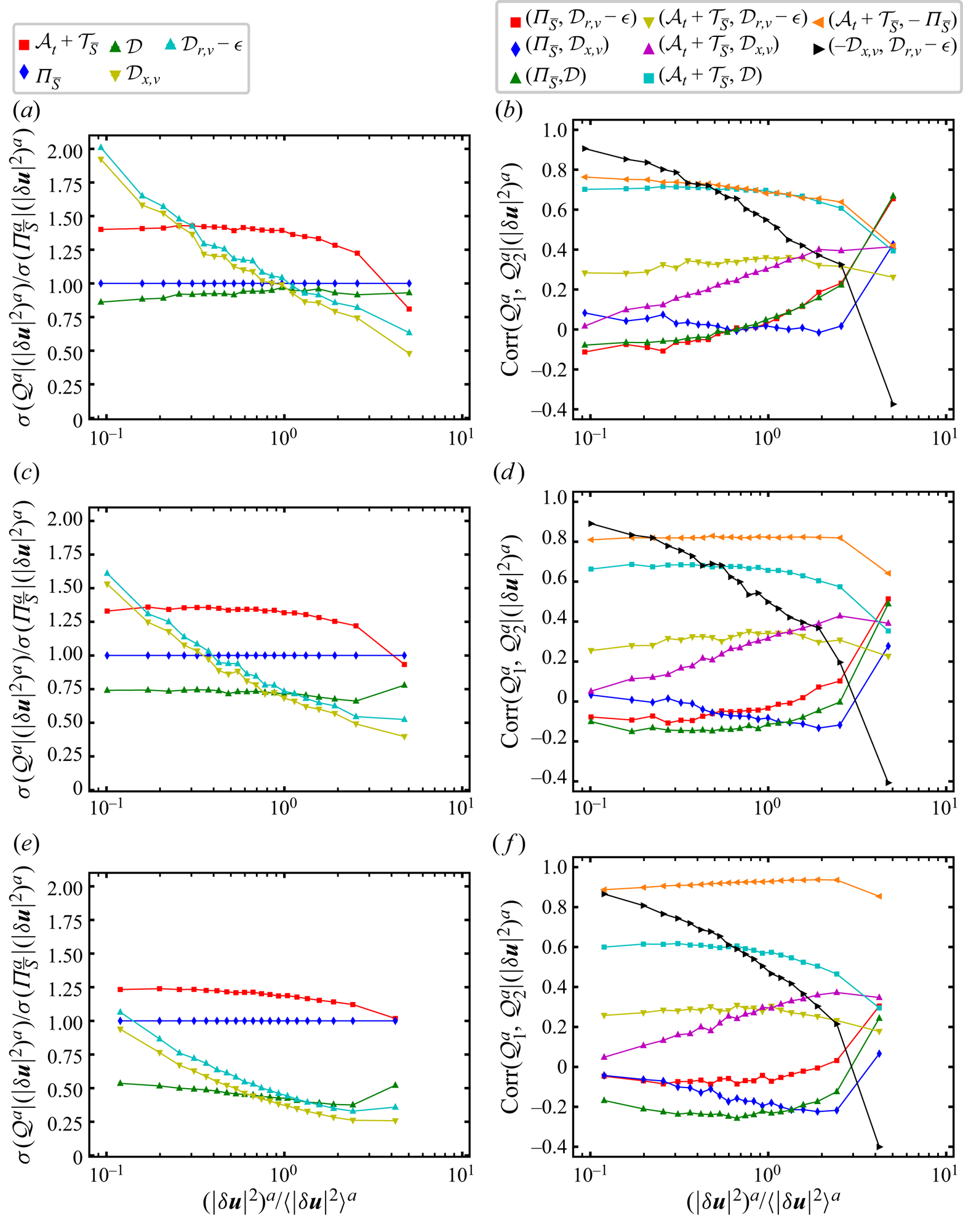
Figure 11. (a,c,e) Conditional standard deviations of various surface-averaged KHMH terms  $\mathcal {Q}^{a}$ for (a)
  $r_{d} = \langle \eta \rangle _t$, (b)
  $r_d = 0.24 \langle \lambda \rangle _t$ and (c)
  $r_{d}= 0.48\langle \lambda \rangle _t$, and (b,d, f) conditional Pearson correlation coefficients of pairs of surface-averaged KHMH terms
  $\mathcal {Q}_{1}^{a}$ and
  $\mathcal {Q}_{2}^{a}$ for (b)
  $r_{d} = \langle \eta \rangle _t$, (d)
  $r_d = 0.24 \langle \lambda \rangle _t$ and ( f)
  $r_{d}= 0.48\langle \lambda \rangle _t$. These standard deviations and correlation coefficients are calculated from spatiotemporal statistics conditioned on various ranges of
  $(\vert \delta \boldsymbol {u}\vert ^2 )^a$ at the
  $r_d$ value of each corresponding plot. The conditioning is identical to that in figure 4: we consider 20 ranges of
  $(\vert \delta \boldsymbol {u}\vert ^2 )^a$ values and the horizontal axes display the average
  $(\vert \delta \boldsymbol {u}\vert ^2 )^a$ values within each
  $(\vert \delta \boldsymbol {u}\vert ^2 )^a$ range normalised by the spatiotemporally averaged small-scale energy
  $\langle |\delta \boldsymbol {u}|^2 \rangle ^a$. Increasing values of
  $(\vert \delta \boldsymbol {u}\vert ^2 )^a$ are therefore from left to right on the horizontal axes.


