


1. Introduction
The stability of liquid filaments, threads or films is an important branch of fluid dynamics. The pioneering research dates back to the discovery of the Plateau–Rayleigh instability, which describes the mechanism governing the breakup of falling fluid streams into smaller droplets due to their surface-tension-driven tendency of minimising their surface area (Plateau Reference Plateau1850). The instability problem becomes more challenging when considering fluid–solid interactions, such as a liquid filament lying upon a solid substrate (Benilov Reference Benilov2009) or within a groove (Sundin, Zaleski & Bagheri Reference Sundin, Zaleski and Bagheri2021), and film dewetting on patterned surfaces (Kim & Kim Reference Kim and Kim2018; Martin-Monier et al. Reference Martin-Monier, Ledda, Piveteau, Gallaire and Sorin2021), where complex interfacial dynamics involving topological breakup, coalescence, etc., are present. A comprehensive understanding of these instabilities and their resulting interfacial morphology is motivated by a wide range of engineering applications. For example, the alteration of interfacial morphology induced by these instabilities has the potential to drive various self- and directed-assembly mechanisms, offering support to advanced manufacturing techniques in microreactors (Yasuga et al. Reference Yasuga, Iseri, Wei, Kaya, Di Dio, Osaki, Kamiya, Nikolakopoulou, Buchmann and Sundin2021) and high-density data storage (Xia & Chou Reference Xia and Chou2009). In addition, knowledge concerning the control of droplet breakup or coalescence resulting from these instabilities is pertinent to technological applications such as bubble generation in microfluidics (Yasuga et al. Reference Yasuga, Iseri, Wei, Kaya, Di Dio, Osaki, Kamiya, Nikolakopoulou, Buchmann and Sundin2021), enhanced oil recovery (Olbricht Reference Olbricht1996) and geological carbon storage (Singh et al. Reference Singh, Bultreys, Raeini, Shams and Blunt2022).
The simplest situation to consider would be a liquid filament or rivulet partially wetting a substrate or a groove, for which the related stability problem has been studied extensively. In an early study, Langbein (Reference Langbein1990) theoretically investigated the stability of an elongated meniscus attached to solid edges at an arbitrary angle using solutions of the Laplace equation and geometric constraints. He established a critical meniscus length beyond which the meniscus becomes unstable. Similarly based on the Laplace equation, Roy & Schwartz (Reference Roy and Schwartz1999) derived a more general stability criterion where the filament stability is guaranteed if the capillary pressure is an increasing function of the filament cross-sectional area. In other words, the stability criterion derived from Laplace equation is also a measure of whether it is energetically favourable for a film to breakup or not (Wilson & Duffy Reference Wilson and Duffy2005). Assuming a shallow liquid film and a small Reynolds number for the flow, the lubrication approximation has also been widely adopted to derive time-dependent equations for film thickness evolution (Hocking Reference Hocking1990; Hocking & Miksis Reference Hocking and Miksis1993). It has been shown that the lubrication approximation yields reasonable predictions for film flows compared with Navier–Stokes solutions (Perazzo & Gratton Reference Perazzo and Gratton2004). This approximation allows for the consideration of gravity and moving contact lines, enabling the modelling of more complex interfacial dynamics. For instance, considering contact angle hysteresis, researchers have thoroughly investigated the competing effects between gravity and surface tension on the stability of an infinite rivulet interacting with an inclined plane (Hocking & Miksis Reference Hocking and Miksis1993; Benilov Reference Benilov2009). Furthermore, numerical frameworks based on the disjoining pressure model (DPM) have been developed for filaments of finite length (Diez & Kondic Reference Diez and Kondic2007; Diez, González & Kondic Reference Diez, González and Kondic2009). The results from using this framework uncovered two dewetting patterns; either the filament shrinks and eventually forms a single droplet if it is short and thick, or it breaks up into several subdroplets. Importantly, a close connection to the Plateau–Rayleigh instability was highlighted, suggesting the same underlying physical mechanisms. Studies employing similar theoretical and numerical techniques but involving other configurations, such as a liquid ring on a solid substrate (González, Diez & Kondic Reference González, Diez and Kondic2013; Edwards et al. Reference Edwards, Ruiz-Gutiérrez, Newton, McHale, Wells, Ledesma-Aguilar and Brown2021) and irregular liquid structures (Huang et al. Reference Huang, Tsou, Chang and Liao2017), have also followed.
At present, more research is focused on liquid structures interacting with confined geometries, such as tubes and corners, owing to their ability to guide a specific fluid phase in a controllable manner, especially in the fields of artificial surfaces and microfluidics. Studies on the stability of liquid structures trapped within wedges and tubes have been reported throughout the literature. For instance, Lv & Hardt (Reference Lv and Hardt2021) explored the stability of a liquid ring with an arbitrary contact angle in circular capillary tubes, deriving an analytical stability limit determining whether the liquid ring would merge into an axisymmetric sessile droplet or a non-axisymmetric liquid plug based on the liquid volume and contact angle. Employing the lubrication approximation, Yang & Homsy (Reference Yang and Homsy2007) theoretically investigated the capillary-induced instability of liquid films attached to a wedge with an emphasis on the effects of contact line dynamics. Similar studies, such as that of Chen, Weislogel & Nardin (Reference Chen, Weislogel and Nardin2006), focused on a wedge with an arbitrary round corner. Despite these efforts, a more in-depth understanding of various aspects of such configurations is still warranted.
2. Cylinder-wrapping corner film
The cylinder-plane-corner geometry is the focus of this work as cylinders are commonly used or encountered in artificial porous media or microfluidic devices (Holtzman & Segre Reference Holtzman and Segre2015; Zhao, MacMinn & Juanes Reference Zhao, MacMinn and Juanes2016; Rabbani et al. Reference Rabbani, Or, Liu, Lai, Lu, Datta, Stone and Shokri2018; Suo Reference Suo2024). The fluid dynamics in the corner regions of such geometries play an essential role in flow patterning. Relevant work has mainly been focused on the process of film formation, i.e. the imbibition along the corners. This so-called corner flow, which emerges as a specific pattern of fluid–fluid displacement in porous media (Primkulov et al. Reference Primkulov, Pahlavan, Fu, Zhao, MacMinn and Juanes2021), occurs under strong imbibition (Zhao et al. Reference Zhao, MacMinn and Juanes2016; Hu et al. Reference Hu, Wan, Yang, Chen and Tokunaga2018) and is also known as the Concus–Finn condition (Concus & Finn Reference Concus and Finn1969). However, the dewetting process has seldom been given attention to. Specifically, once beyond the Concus–Finn condition, capillary-induced instability may occur in the formed wrapping films. The relevant knowledge is crucial for a practical purpose as highlighted in our prior work (Suo et al. Reference Suo, Zhao, Bagheri, Yu and Gan2022). Artificial textured surfaces, proposed for anti-icing and antifouling, often feature patterned microstructures within which stagnant stain films are undesirable. Such capillary-induced instability is expected to drive the trapped films to break up into distributed small drops, facilitating easy purging of the stain liquid. Understanding the underlying mechanisms is essential for optimising the design of functional surfaces.
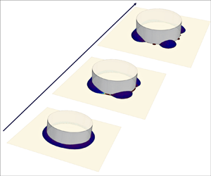
A film–cylinder system is presented in figure 1(a). It shows a settled film on a flat surface at a contact angle of  $30^{\circ }$ which is also wrapped around a cylinder at a contact angle of $90^{\circ }$. An example of how the breakup of such a film evolves, obtained using a volume-of-fluid (VOF) simulation, is shown in figure 1(b). One can see how the perturbation in the film grows over time and finally causes it to break up into four major satellite droplets labelled on the final state in figure 1(b). Figure 2 depicts a conceptual examination of this instability mechanism. The perturbation is assumed as a superposition of sinusoidal components with various wavenumbers. Considering only a single component where the wavenumber is five, in figure 2(a) the perturbed interface shows two types of regions which are convex and concave with respect to the equilibrium state. At the convex region (crest), the curvature ( $1/R^c_1$) is positive, yielding a larger capillary pressure compared with that at the concave region (neck) where the curvature ( $1/R^n_1$) is negative. Consequently, the liquid tends to be transported from the convex to the concave region, eventually returning the film to its equilibrium state. However, the capillary pressure, as determined by the Young–Laplace equation, also depends on the curvatures in the other principal direction, i.e. $1/R^c_2$ in figure 2(b) and $1/R^n_2$ in figure 2(c), which are both positive. The curvature ( $1/R^c_2$) in the convex region may become smaller whereas the curvature ( $1/R^n_2$) in the concave region may become larger due to the perturbation. Thus, the latter effect can counteract the former and prevent the liquid from flowing from the convex to the concave regions. These two effects are determined by the wavenumber, wettability conditions and film size. If they cannot balance each other out, the perturbed component would grow or decay over time, corresponding to a positive or negative growth rate. In general, the component with the maximum growth rate would dominate the instability process and eventually pinch the film into satellite droplets, the number of which can be predicted by the corresponding wavenumber as shown in figure 1(b).

Figure 1. (a) Numerical realisation of a liquid film wrapping a cylinder. (b) Top views of the morphology evolution from the initial state to final breakup. The ratio of film size on the cylinder radius is 0.22; the contact angle on the cylinder and the substrate is  $90^{\circ }$ and $30^{\circ }$, respectively.

Figure 2. Schematic of a perturbed corner film from two principal directions: (a) top view; (b) and (c) side views corresponding to the convex and concave region, respectively.
Modelling the development of this instability and predicting the consequent morphology patterns would draw a quantitative picture of the combined effects on the film stability. As such, our work focuses on two questions; first, under what conditions does the corner film become unstable; and, second, how many satellite droplets are formed once the instability occurs. In particular, the latter further determines the droplet size and distribution. The outcomes of this study will have implications for the design of artificial surfaces and other engineering processes requiring the self-assembly of soft matters. The paper is organised as follows. In § 3, the long-wave theory scheme is used to formulate the governing equation of the film thickness and introduce the corresponding boundary conditions. The equilibrium profile is solved for a certain corner condition, based on which we perform a standard linear stability analysis (LSA) to obtain the growth rate. The dependence of growth rate and characteristic wavenumbers on the corner conditions is then thoroughly investigated. To gain more understanding of interfacial dynamics during the film breakup process and validate the LSA predictions, a numerical scheme using the DPM for directly tracking the evolution of film morphology is developed in § 4. In addition, numerical simulations involving solutions of the Navier–Stokes equations for two-fluid systems using the VOF method, which abandon the assumptions used in LSA and DPM, are conducted in § 5. We ultimately demonstrate to what extent the simplified theoretical model can explain the phenomena observed in the VOF simulations and explain the applicability of the LSA predictions.
3. Linear stability analysis
We first develop a mathematical model for describing the evolution of a flat and thin corner film, obtain its equilibrium state and finally perform LSA. Figure 3 shows a schematic of the problem under consideration, a liquid film wrapping a vertical cylinder, along with the relevant geometric parameters including the cylinder radius  $r_1$, wetting radius $r_w$ and height $h_w$, contact angle on the cylinder $\theta _1$ and on the bottom wall $\theta _2$.

Figure 3. A schematic of a corner liquid film around a wall-mounted cylinder and the relevant geometric parameters.
3.1. Governing equations
Limiting the configuration to a thin and flat film, we can describe the flow within the long-wave theory framework, also known as the lubrication approximation, which requires: (1) the film is thin ( $r_w\ll r_1$); (2) the profile slope is small everywhere ( $\theta _1 \to 90^{\circ }$ and $\theta _2 \to 0^{\circ }$). In the reported works (Perazzo & Gratton Reference Perazzo and Gratton2004; Mahady et al. Reference Mahady, Afkhami, Diez and Kondic2013), comparison with Navier–Stokes simulations indicates that the theoretical solution can provide reasonable results for slope angles smaller than $45^{\circ }$. Therefore, we limit the parameter space to $\theta _1\in [75^{\circ }, 90^{\circ }]$, $\theta _2\in [15^{\circ }, 45^{\circ }]$ and $r_w/r_1\in [0.12, 0.30]$. In addition, we assume that the characteristic size of the liquid film is smaller than the capillary length $l_c=\sqrt {\gamma /\rho g}$, where $\rho g$ is the specific weight of the liquid and $\gamma$ is the surface tension, so that gravity effects can be neglected. To address the so-called ‘contact-line singularity’ (Shikhmurzaev Reference Shikhmurzaev2006; Savva & Kalliadasis Reference Savva and Kalliadasis2011), we relax the no-slip condition at the wall boundary by using the Navier-slip boundary condition, which allows the contact line to slip, i.e.
 \begin{equation} u_{r, \phi}|_{z=0} = \frac{\ell}{3}\frac{\partial u_{r, \phi}}{\partial z}, \end{equation}
where  $\ell$ is the prescribed slip length. Combined with this boundary condition, the governing equation regarding the film thickness $h$ is built in a cylindrical coordinate system ( $r$,
$r$,  $\phi$, $z$). Non-dimensionalising the lengths with $r_{1}$ and time with $6\mu r_{1}/{\gamma }$, a characteristic time scale for the evolution of the liquid film breaking or recovering from a perturbation, where $\mu$ is the liquid viscosity, gives (Hocking & Miksis Reference Hocking and Miksis1993)
 \begin{equation} \frac{\partial h}{\partial t}+\boldsymbol{\nabla} \boldsymbol{\cdot}[h^{2}(h+\ell) \boldsymbol{\nabla} \nabla^{2} h]=0. \end{equation}
At the contact lines on the cylinder ( $r=r_1$) and bottom wall ( $r=r_1+r_w$), we impose the Dirichlet boundary conditions expressed as
 $$\begin{gather} h(r_1, t)=h_w(\phi, t ), \end{gather}$$
 $$\begin{gather}h(r_1+r_w (\phi, t), t )=0; \end{gather}$$
and the Neumann boundary conditions stemming from the wall wettability, i.e. the given contact angles,
 $$\begin{gather} \left.\frac{\partial h}{\partial r} \right|_{r=r_1} ={-}\cot\theta_1, \end{gather}$$
 $$\begin{gather}\left.\frac{\partial h}{\partial r} \right|_{r=r_w+r_1} ={-}\tan\theta_2. \end{gather}$$
The solution of (3.2)–(3.4) is assumed to be a superposition of an equilibrium solution  $h_{0}(r, \phi )$ and a perturbation $h_{1}(r, \phi, t)$,
 \begin{equation} h(r, \phi, t)=h_{0}(r, \phi )+\epsilon h_{1}(r, \phi, t), \end{equation}
where  $\epsilon \ll 1$. Substituting (3.5) into (3.2), we obtain the static equation for $h_0$,
 \begin{equation} \nabla^2 h_0={-}p, \end{equation}
where  $p$ is a constant representing the capillary-induced pressure difference from the surrounding gas pressure. Neglecting the higher-order term $O(\epsilon ^2 )$, the perturbation equation becomes
 \begin{equation} \frac{\partial h_1}{\partial t}+\boldsymbol{\nabla} \boldsymbol{\cdot}[h_{0}^{2}(h_{0}+\ell) \boldsymbol{\nabla}(\nabla^{2} h_{1})]=0. \end{equation}
3.2. Equilibrium solution
Considering an axisymmetric solution to (3.6) gives
 \begin{equation} h_{0}(r)={-}\frac{p r^{2}}{4}+c_{1} \ln r+c_{2}, \end{equation}
where the unknown parameters  $c_1$, $c_2$, $p$ and $h_{w0}$ are determined by the boundary conditions (3.3) and (3.4), assuming $r_{w0}$ is given. The parameters are given by
 $$\begin{gather} c_1 = \frac{r_2}{r_2^2 - 1} ( \tan \theta_2 - r_2 \cot \theta_1 ), \end{gather}$$
 $$\begin{gather}c_2 = \frac{r_2}{2(r_2^2 - 1 )} [2\ln r_2( r_2\cot \theta_1 - \tan \theta_2) + r_2(r_2 \tan \theta_2 - \cot \theta_1)], \end{gather}$$
 $$\begin{gather}p = 2 \frac{r_2 \tan\theta_2 - \cot \theta_1}{(r_2^2 - 1)}, \end{gather}$$
 $$\begin{gather}h_{w0} = c_{2}-\frac{1}{4} p, \end{gather}$$
where  $r_2 = r_1 + r_{w0}$. The wettability condition ( $\theta _1$ and $\theta _2$) and initial film size ( $r_{w0}$), compose the corner condition, which completely determines the equilibrium interfacial shape. Figure 4 compares the equilibrium profiles for different $\theta _1$, $\theta _2$, and $r_{w0}$. With a fixed $r_{w0}$, $\theta _1$ and $\theta _2$ directly change the interfacial curvature. As shown in figures 4(a) and 4(b), the smaller $\theta _1$ and $\theta _2$ are (the more hydrophilic the solid walls are) the smaller the curvature of the meniscus becomes. When the wettability condition is fixed, figure 4(c) shows that with increasing $r_{w0}$ the changes in $h_{w0}$ are relatively smaller, resulting in flatter corner films.

Figure 4. Equilibrium interfacial profiles for: (a)  $r_{w0}=0.26$, $\theta _2 = 30^{\circ }$ and $\theta _1 = 75^{\circ }, 82.5^{\circ }$ and $90^{\circ }$;(b) $r_{w0}=0.26$, $\theta _1 = 82.5^{\circ }$ and $\theta _2 = 15^{\circ }, 30^{\circ }$ and $45^{\circ }$; and (c) $\theta _1 = 90^{\circ }$, $\theta _2 = 30^{\circ }$ and $r_{w0}=0.12, 0.21$ and $0.30$.
3.3. Eigenvalue problem
The LSA is conducted using an equilibrium solution for a certain corner condition. Since the circumferential length of the film is much larger than its length along the  $r$ and $z$ axes ( $r_w \approx h_w\ll 2{\rm \pi} r_1$), we can assume the perturbation is a periodic wave along the $\phi$ axis. The perturbation $h_1$ thus takes the following form:
 \begin{equation} h_{1}(r, \phi, t)=\hat{h}_{1}(r) \, {\rm e}^{\mathrm{i} (n \phi - \lambda t )}. \end{equation}
In (3.10),  $n$ is the azimuthal wavenumber. Importantly, though $n$ is real, only the integer values of $n$ are physically meaningful as they correspond to the number of formed fingers which is related to the satellite droplets in the final state. In addition, $\lambda = \mathrm {i} \sigma + \omega$ is the complex frequency composed of the growth rate $\sigma$ and the phase speed $\omega$. Consequently, the perturbation at the boundaries has the following form:
 $$\begin{gather} h_w(\phi, t) = h_{w0}+\epsilon\xi_1\, {\rm e}^{\mathrm{i} (n \phi - \lambda t)}, \end{gather}$$
 $$\begin{gather}r_w(\phi, t) = r_{w0}+\epsilon\xi_2\, {\rm e}^{\mathrm{i} (n \phi - \lambda t)}, \end{gather}$$
where  $\xi _1$ and $\xi _2$ are two coefficients determined by the boundary conditions. Substituting (3.10) into (3.7), we obtain the eigenvalue problem,
 \begin{equation} \mathcal{L}(\hat{h}_1)=\mathrm{i}\lambda \hat{h}_1, \end{equation}
where
 \begin{equation} \mathcal{L} (\hat{h}_1 ) = \hat{c}_4(r, n) \hat{h}_{1, rrrr} + \hat{c}_3(r, n) \hat{h}_{1, rrr} + \hat{c}_2(r, n) \hat{h}_{1, rr}+ \hat{c}_1(r, n) \hat{h}_{1, r} + \hat{c}_0(r, n) \hat{h}_{1}. \end{equation}
The coefficients  $\hat {c}_0$– $\hat {c}_4$ can be expressed explicitly as
 $$\begin{gather} \hat{c}_4 = H_0, \end{gather}$$
 $$\begin{gather}\hat{c}_3 = 2 H_0 /r+H_{0r}, \end{gather}$$
 $$\begin{gather}\hat{c}_2 = H_{0r} /r -(2n^2+1)H_0/r^2, \end{gather}$$
 $$\begin{gather}\hat{c}_1 = (2n^2+1)H_0 /r^3 - (n^2+2)H_{0r} /r^2+H_{0r} (h_{0rr}/r+h_{0rrr})/ h_{0r}, \end{gather}$$
 \begin{gather} \hat{c}_0 = H_{0r}h_{0rrrr}+(r H_1 h_{0r}+2H_{0r}/h_{0r})h_{0rrr}/r\nonumber\\ \qquad\quad +(r H_1 h_{0r}-H_{0r}/h_{0r})h_{0rr}/r^2 - 2H_1(h_{0r}/r)^2 \nonumber\\ \qquad\qquad\quad\quad\qquad +(2n^2+1)h_{0} H_{0r}/r^3+n^2(n^2-4)h^2_{0}(h_{0}+1)/r^4, \end{gather}
where  $H_0=h^2_0(h_0+\ell$) and $H_1=2(3h_0+\ell )$. The boundary conditions on $\hat {h}_1$ can be implemented by substituting (3.10) and (3.11) into (3.3) and (3.4) and only keeping the linear terms. Specifically, on the cylinder wall,
 $$\begin{gather} h_0(r_1)+\epsilon\hat{h}_1(r_1)\, {\rm e}^{\mathrm{i} (n \phi - \lambda t)}=h_{w0}+\epsilon\xi_1\, {\rm e}^{\mathrm{i} (n \phi - \lambda t)}, \end{gather}$$
 $$\begin{gather}h_0'(r_1)+\hat{h}_1'(r_1)\, {\rm e}^{\mathrm{i} (n \phi - \lambda t)}={-}\cot \theta_1; \end{gather}$$
and on the bottom wall,
 $$\begin{gather} h_0(r_2) + \epsilon\xi_2 h'_0(r_2)\, {\rm e}^{\mathrm{i} (n \phi - \lambda t)} + \epsilon\hat{h}_1(r_1+r_w)\, {\rm e}^{\mathrm{i} (n \phi - \lambda t)}=0, \end{gather}$$
 $$\begin{gather}h_0'(r_2) + \epsilon\xi_2 h''_0(r_2)\, {\rm e}^{\mathrm{i} (n \phi - \lambda t)}+ \epsilon\hat{h}'_1(r_1+r_w)\, {\rm e}^{\mathrm{i} (n \phi - \lambda t)}={-}\tan\theta_2. \end{gather}$$
The unknown amplitudes  $\xi _1$ and $\xi _2$ can be eliminated by solving (3.15) and (3.16). The explicit expression for the boundary conditions then become
 $$\begin{gather} \hat{h}_1'(r_1) = 0, \end{gather}$$
 $$\begin{gather}\hat{h}'_1(r_1+r_{w})=\hat{h}_1(r_1+r_{w})\frac{h''_0(r_1+r_{w})}{h'_0(r_1+r_{w})}. \end{gather}$$
For a given  $n$, to solve (3.12), we map the $r$ space ( $r_1 \leq r \leq r_1+r_{w}$) onto the $\zeta$ space ( $-1 \leq \zeta \leq 1$) by
 \begin{equation} r=r_1+\frac{r_{w}}{2}(\zeta+1),\end{equation}
and correspondingly  $\hat {h}_1(r)$ is replaced by $g(\zeta )$. This gives the eigenvalue problem (3.12) in terms of $\zeta$,
 \begin{equation} \mathcal{L}(g)=\mathrm{i}\lambda g,\end{equation}
and  $g(\zeta )$ can be discretised as
 \begin{equation} g(\zeta)=\sum_{i=1}^{N}\beta_i\varphi_i,\end{equation}
where  $\varphi _i$ are an orthogonal basis and $\beta _i$ are the spectral coefficients. To make $\varphi _i$ satisfy the boundary conditions at $\zeta =\pm 1$, a linear combination of Chebyshev functions $T_i$ is adopted to form $\varphi _i$,
 \begin{equation} \varphi_i = T_{3i-3} + a_i T_{3i-2} + b_i T_{3i-1},\end{equation}
where the coefficient  $a_i$ and $b_i$ can be determined by substituting (3.21) into boundary conditions (3.17). The Gauss–Lobatto grid is adopted to discretise the radial space
 \begin{equation} \zeta_i =\cos\left(\frac{{\rm \pi} i}{N-1}\right), \quad i=1, 2,\ldots, N-2.\end{equation}
Finally, (3.12) is transformed into a generalised matrix eigenvalue problem,
 \begin{equation} \boldsymbol{\mathsf{U}}\boldsymbol{\beta}=\lambda \boldsymbol{\mathsf{V}} \boldsymbol{\beta}, \end{equation}
where  $U_{i,j} = \mathcal {L}(\zeta _i, \varphi _j)$ and $V_{i, j}=\varphi _j(\zeta _i)$.
3.4. Perturbation dynamics
By solving the eigenvalue problem, the dependence of  $\lambda$ on $n$ is obtained. Since the solved phase speed $\omega$ of the dominating perturbation modes equals zero, indicating that they are periodic structures that can grow or decay, we only discuss the growth rate $\sigma$ for the following. A resolution sensitivity test determined that $N=200$ is required to guarantee a convergent solution, as shown in figure 5(a). In the nonlinear regime, the interactions between various modes would generally occur and, thus, further assessment of which mode would dominate is needed. However, as shown in figure 5(b), the second largest $\sigma$ is negative and much smaller than the first one. It suggests that for this problem, only the leading mode of the LSA would dominate and the largest $\sigma$ is the one we should focus on. For what follows, $\sigma$ represents the largest growth rate unless otherwise specified. The growth rate curve, $\sigma$ vs $n$, quantifies the stability of the film–cylinder system to various perturbations. Positive $\sigma$ indicates exponential growth of a perturbation whereas a negative growth rate means that the film is stable with respect to the imposed perturbation. The rationale of the growth rate curve shape can be explained using figure 2. Overall, with the wavenumber increasing, the in-plane curvatures, i.e. the stabilising effects monotonically increases, while the out-of-plane curvatures, i.e. the destabilising effects become significant only for a specific range of small-value wavenumbers. Therefore, for the growth rate, a peak appears at a small-value wavenumber and it becomes negative eventually with the increasing wavenumber. The cut-off ( $0$,
$0$,  $n_{zero}$) and peak ( $\sigma _{max}$, $n_{max}$) azimuthal wavenumbers are used for the following to characterise the film stability. Specifically, the cut-off point, $n_{zero}$, corresponds to the maximum possible number of fingers for a given baseflow. Should $\sigma$ become negative and $n>n_{zero}$, the corresponding perturbation would become suppressed. As such, $n_{zero}$ defines the boundary between the stable and unstable regime. The peak growth rate, $\sigma _{max}$, corresponds to $n_{max}$ and indicates that the perturbation would grow the fastest and have the largest likelihood of dominating the instability process. Therefore, $n_{max}$ is approximately the expected number of emerging fingers when the film is stimulated by a random perturbation containing a wide range of wavenumbers. In addition, the growth rate curves for various slip lengths, i.e. $\ell =10^{-2}$, $\ell =10^{-3}$ and $\ell =10^{-4}$, are compared as shown in figure 5(c). Though $\ell$ impacts the values of $\sigma$, it does not change the $n_{max}$ and $n_{zero}$. Moreover, the curves for $\ell =10^{-3}$ and $\ell =10^{-4}$ are almost overlapped, suggesting that the effects of $\ell$ can be neglected when $\ell$ is small enough. Thus, for what follows, we set $\ell$ as $10^{-3}$ and focus on the effects of the corner conditions. Figure 6 shows the growth rate curves for the corner conditions shown in figure 4. Regarding the wettability effects, as $\theta _1$ increases from $75^{\circ }$ to $90^{\circ }$ in figure 6(a), the growth rate curve tends to be flatter, suggesting that $n_{max}$ and $n_{zero}$ increase while $\sigma _{max}$ decreases.

Figure 5. (a) Resolution sensitivity of the largest  $\sigma$ on the grid number $N$ for $r_{w0}=0.26$, $\theta _1=90^{\circ }$ and ${\theta _2=30^{\circ }}$. (b) The corresponding largest and second largest growth rate, i.e. $\sigma _1$ and $\sigma _2$ vs $n$ with $N=200$. (c) The comparison of the largest $\sigma$ for various slip lengths.

Figure 6. Growth rate curves for: (a)  $r_{w0}=0.26$, $\theta _2 = 30^{\circ }$ and $\theta _1 = 75^{\circ }, 82.5^{\circ }$ and $90^{\circ }$; (b) $r_{w0}=0.26$, ${\theta _1 = 82.5^{\circ }}$ and $\theta _2 = 15^{\circ }, 30^{\circ }$ and $45^{\circ }$; and (c) $\theta _1 = 90^{\circ }$, $\theta _2 = 30^{\circ }$ and $r_{w0}=0.12, 0.21$ and $0.30$. The arrows show the direction of increasing $\theta _1$ in (a), $\theta _2$ in (b) and $r_{w0}$ in (c).
In contrast to the effect of  $\theta _1$, $\sigma _{max}$ increases with $\theta _2$, as shown in figure 6(b). González et al. (Reference González, Diez and Kondic2013) suggested an approximate scaling $\sigma \propto \tan ^3 \theta _2$ for a liquid ring on a solid substrate, which applies to cases where $\theta _1 = 90^{\circ }$ as shown in figure 7(a). However, figure 7(b) shows that this scaling does not hold once $\theta _1$ takes other values, e.g. $75^{\circ }$. Since the eigenvalue problem is governed by the coefficients $\hat {c}_i$ in (3.13) and $\hat {c}_i \sim h_0^3$, the scaling would require that $h_0 \sim \tan \theta _2$. According to (3.9), this requirement will only be satisfied when $\theta _1 \to 90^{\circ }$ and therefore $\cot \theta _1 \to 0$.

Figure 7. Scaled growth rate  $\sigma /\tan ^3\theta _2$ for the cases with $r_{w0}=0.26$: (a) $\theta _1 = 90^{\circ }$ and (b) $\theta _1 = 75^{\circ }$. The peak and cut-off wavenumber are marked by black circles in (a).
Regarding the effect of the film size, as shown in figure 6(c), with increasing  $r_{w0}$, both $n_{max}$ and $n_{zero}$ decline, suggesting that a thick corner film is less susceptible to high-wavenumber perturbations. Increasing $r_{w0}$ would weaken the relative difference between the curvatures at the crest, $1/R^c_2$, and the neck, $1/R^n_2$, which drives the film to break up, since the corner film becomes flatter as the film size becomes larger (see figure 4a). However, the curvature difference of $1/R^c_1$ and $1/R^n_1$, which suppresses the instability, is comparatively less influenced by $r_{w0}$. Thus, the thicker the film becomes, the more stable it would be.
3.5. Characterisation of film stability
A complete picture for characterising the film stability in the parameter space  $\theta _1\in [75^{\circ }, 90^{\circ }]$, $\theta _2\in [15^{\circ }, 45^{\circ }]$ and $r_{w0}\in [0.12, 0.30]$ can now be provided to answer the questions posed at the beginning. Namely, under what conditions does the corner film become unstable and how many satellite droplets are formed once the instability occurs. Here, we assume that the number of fingers predicted from LSA is equal to the number of satellite droplets in the final state.
We first investigate the marginal stability corresponding to the critical condition under which the film would become unstable. This can be characterised by  $n_{zero}$ and $\sigma _{max}$. The solid lines in figures 8(a), 8(c) and 8(e) depict $n_{zero}$ vs $r_{w0}$ and distinguish the regions of stability (upper) and instability (lower). The stable region is modified by the wall wettability. As $\theta _1$ and $\theta _2$ decrease, the stable region becomes enlarged. In particular, for $\theta _1=90^{\circ }$, the condition corresponding to $n_{zero}$ becomes independent of $\theta _2$ and the curves for various $\theta _2$ collapse as one in figure 8(c) owing to the scaling law mentioned previously in connection with figure 7(a). With increasing $r_{w0}$, $n_{zero}$ decreases and eventually approaches a value of $n=6$ or $n=7$. This seems to suggest that the corner film tends to be more stable when it becomes thicker, but full stability cannot be achieved. However, due to the assumption of the long-wave theory, i.e. $r_{w0} \ll r_1$, the LSA may not lead to accurate predictions if the corner film is too thick.

Figure 8. Stability curves for  $\theta _1=$ $75^{\circ }$ (a,b), $82.5^{\circ }$ (c,d) and $90^{\circ }$ (e,f). (a,c,e) Curves of $n_{zero}$– $r_{w0}$ with various $\theta _2 \in [15^{\circ }, 22.5^{\circ }, 30^{\circ },37.5^{\circ },45^{\circ }]$. (b,d,f) Equilibrium profiles with $r_{w0} = 0.30$ and various $\theta _2$.
Focus is now placed on predictions of the expected number of satellite droplets, which correspond to the perturbation mode with the maximum growth rate. Figure 9 shows the contours of  $\sigma _{max}$ and $n_{max}$, with the latter indicating the expected number of satellite droplets. Note that $\sigma _{max}$ is mainly controlled by wall wettability and only slightly affected by the film size. Figures 9(b), 9(d) and 9(f) show that the expected number of satellite droplets generally decreases with $r_{w0}$ while ranging from 4 to 9.

Figure 9. Contours of  $\sigma _{max}$ (a,c,e) and $n_{max}$ (b,d,f) for $\theta _1= 75^{\circ }$ (a,b), $\theta _1=82.5^{\circ }$ (c,d) and $\theta _1=90^{\circ }$ (e,f) in the parameter space of $\theta _2$ and $r_{w0}$. The values of contour lines in (a,c,e) are $[1, 2, 3, 4, 5, 6, 7, 8]$.
Overall, the film stability can be characterised by the growth rate curve obtained from the LSA. Specifically, the postinstability pattern, including the maximum and most probable number of fingers, can be predicted by  $n_{zero}$ and $n_{max}$, respectively. The film size $r_{w0}$ plays the most important role in determining the marginal stability and the postinstability pattern of a corner film. The thicker the film is, the less susceptible it becomes to perturbations of a higher wavenumber. The wall wettability including $\theta _1$ and $\theta _2$ mainly influence $\sigma _{max}$ while having a secondary influence on $n_{zero}$ and $n_{max}$. Importantly, although the LSA is effective for predicting early stage nonlinear dynamics, specifically the initial finger formation, a critical question arises: to what degree can the predicted fingers accurately represent the satellite droplets of the final state? In the subsequent sections, we compare the LSA prediction against the numerical results obtained using the DPM and VOF simulations to assess the LSA's capability to predict the postinstability development, particularly when nonlinear effects become involved in the breakup stage.
4. Disjoining pressure model
Rather than using the Navier-slip boundary condition to address stress singularity at the contact line and directly applying contact angles, as was done in § 3, a precursor film is assumed and the wettability condition on the walls can be represented via a disjoining pressure  $\varPi (h)$ (Diez & Kondic Reference Diez and Kondic2007; Savva & Kalliadasis Reference Savva and Kalliadasis2011; Kondic et al. Reference Kondic, González, Diez, Fowlkes and Rack2020),
 \begin{equation} \frac{\partial h}{\partial t}+\boldsymbol{\nabla} \boldsymbol{\cdot}[h^{3} \boldsymbol{\nabla} \nabla^{2} h+h^{3}\boldsymbol{\nabla}\varPi(h)]=0. \end{equation}
The most commonly used form of  $\varPi (h)$ is adopted here (Mitlin & Petviashvili Reference Mitlin and Petviashvili1994; Schwartz Reference Schwartz1998),
 \begin{equation} \varPi(h) = Kf(h)=K\Bigg[ \left( \frac{h_*}{h} \right)^a- \left(\frac{h_*}{h} \right)^b\Bigg], \end{equation}
where  $f(h)$ represents liquid–solid repulsion and attraction with exponents $a>b>1$. Throughout the literature, the dynamic effects of different exponent pairs $(a,b)$ including $(9, 3)$, $(4, 3)$ and $(3,2)$ have been discussed (Craster & Matar Reference Craster and Matar2009; Kondic et al. Reference Kondic, González, Diez, Fowlkes and Rack2020). In this work, we adopt $(3,2)$ (Schwartz & Eley Reference Schwartz and Eley1998). This liquid–solid interaction leads to a thickness $h_*$ at which the repulsive and attractive forces are balanced. $h_*$ is related to a precursor film thickness (Savva & Kalliadasis Reference Savva and Kalliadasis2011), which under realistic conditions is of nanoscale thickness. Hence, $h_*$ should be extremely small. Computationally, the grid spacing must also be close to $h_*$ to guarantee numerical convergence. To maintain a reasonable level of computational cost, we adopt $h_*=10^{-3}$. The constant $K=2(1-\cos \theta _*)/h_*$, where $\theta _*$ is related to the contact angle. Due to interface relaxation, the contact angle measured from the equilibrium state would be smaller than $\theta _*$. Finally, the governing equation (3.2) becomes
 \begin{equation} \frac{\partial h}{\partial t}+\boldsymbol{\nabla} \boldsymbol{\cdot}[h^{3} \boldsymbol{\nabla} \nabla^{2} h]+ K\boldsymbol{\nabla} \boldsymbol{\cdot} (h^3 f'(h)\boldsymbol{\nabla} h)=0. \end{equation}
Equation (4.3) is solved for the domain shown in figure 10 with the following boundary condition on the cylinder wall:
 \begin{equation} \boldsymbol{\nabla} h \boldsymbol{\cdot} \boldsymbol{n} ={-}\cot \theta_1, \end{equation}
where  $\boldsymbol {n}$ is the unit normal vector, and on the domain boundary
 \begin{equation} h = h_*. \end{equation}
To prevent the outer boundary from affecting the film evolution, the domain size,  $r_b$, is set two times larger than $r_1$.

Figure 10. Schematic of the numerical model for the DPM, including a computation domain lying between the cylinder wall and the domain boundary. Here,  $r_1$ is the cylinder radius and $r_b$ defines the domain size.
First, an equilibrium profile needs to be obtained. Specifically, a solution obtained from (3.8) is elevated by  $h_*$, thereby guaranteeing that $h\geq h_*$. This modified solution is taken as an initial profile. It evolves by solving (4.3) in an axisymmetric domain until a steady state is achieved. The final steady state may be different from the assumed initial profile from (3.8) because the contact line would slide along the precursor film. To match the LSA and DPM, it is necessary to re-evaluate the corner condition used in the LSA to conform to the steady solution from the DPM. We keep the liquid volume $V$,
$V$,  $r_{w0}$ and $\theta _1$ fixed, then adjust $\theta _2$ to fit the steady profile of the DPM. One case is shown in the inset of figure 11(b) where initially $r_{w0}=0.27$, $\theta _1 = 90^{\circ }$ and $\theta _* = 60^{\circ }$, but the final fitting yields $\theta _2 = 33^{\circ }$. Once the equilibrium profile is obtained, we add a perturbation $\epsilon h_1(\phi )|_{t=0}$ and solve (4.3) for
 \begin{equation} h(r, \phi)|_{t=0} =h_0(r)+\epsilon h_1(\phi)|_{t=0}. \end{equation}
Finally, we obtain the time evolution of  $h$, from which the growth rate $\sigma$ can be estimated as
 \begin{equation} \epsilon \overline{h}_1(t) = \sqrt{\int_{\varOmega} [h(r, \phi, t)-h_0(r)]^2 \, {\rm d} \varOmega }. \end{equation}
Here,  $\varOmega$ is the computation domain as shown in figure 10.

Figure 11. (a) The perturbation growth for the case with  $r_{w0}=0.27$, $\theta _1 = 90^{\circ }$ and $\theta _* = 60^{\circ }$. (b) The comparison of growth rate between DPM and LSA. The inset in (b) shows the steady profile used in the DPM and correspondingly the equilibrium solution with $\theta _2 = 33^{\circ }$ for the LSA. (c) The evolution of film morphology from the instability occurrence to film breakup.
4.1. Single-mode perturbations
We start by investigating the dynamics of a corner film triggered by single-mode perturbations, i.e.
 \begin{equation} \epsilon h_1(\phi)|_{t=0} =A_n \cos (n\phi). \end{equation}
The perturbation amplitude  $A_n = 10^{-4}$ is small enough to guarantee that linearity dominates in the initial stage. The evolution of $\epsilon \overline{h}_1$ for $n=1,\ldots,7$ are shown in figure 11(a). After a short oscillation period, the perturbation grows exponentially and, thus, the growth rate for each wavenumber can be obtained by linear fitting. As shown in figure 11(b), results of the LSA and DPM are in good agreement around $n_{max}$ and demonstrate a consistent trend. We do not expect a perfect quantitative agreement due to the difference in modelling contact line movement. Specifically, in the DPM the ‘contact line’ slides on the precursor film so that the interface near the wall surface appears as an asymptotic slope rather than a sharp angle, whereas in the proposed theoretical model the contact line movement is through wall slip.
The film instability process exhibits linear behaviour initially, with the number of emerging fingers being consistent with the wavenumber  $n$, as is shown in the first column of figure 11(c). However, nonlinearity dominates the final phase of the evolution and results in a more complex film morphology. Taking $n=3$ as an example, a slim and long film forms at each neck region which connects two neighbouring fingers. At $t=5$, the connecting film breaks up at its two ends and then forms a secondary droplet. Eventually, in addition to three major droplets, three secondary droplets appear in between the major ones. For $n=4$, the connecting films become relatively shorter, resulting in smaller secondary droplets. Thus, the Laplace pressure of the secondary droplet becomes much larger than that of the neighbouring major droplet, and this pressure difference drives the liquid to fast flow from the secondary droplets to the major ones. Eventually, secondary droplets only appear temporally and are absorbed by neighbouring major ones. For $n=5$, the connecting film is too short to form a secondary droplet and only major satellite droplets appear during the breakup.
4.2. Random perturbations
In general, perturbations are of a random nature covering a wide range of wavenumbers. We consider a superposition of  $N$ individual single-mode perturbations,
 \begin{equation} \epsilon h_1(\phi)|_{t=0} =\sum_{n=0}^{N} A_n \cos (n\phi), \end{equation}
where  $A_n$ are random amplitudes within $[-A_{max}, A_{max}]$ with $A_{max}=10^{-4}$ and $N=100$. Ten samples of $\epsilon h_1(\phi )|_{t=0}$ are generated and superimposed on the baseflow shown in the inset of figure 11(b). According to the LSA, the perturbation mode with $n=5$ has the maximum growth rate and thus five fingers are expected to formed. However, for this case, the four-finger and the five-finger pattern are equally likely to occur since the difference between the first and second largest growth rate is small, i.e. $\sigma = 1.16$ for $n=4$ whereas $\sigma = 1.25$ for $n=5$. Perturbation energy obtained from the DPM is shown in figure 12(a) for the two perturbations. Snapshots of the corner film evolving after being perturbed are presented in figure 12(b). Due to randomness, the film breakup at the neck regions is asynchronous, unlike single-mode perturbations, and therefore the final film morphology loses symmetry. Consequently, the connecting films have different lengths, which in turn causes the emerging secondary droplets to appear at random between two major droplets. For example, as shown in the third column of figure 12(b) for $n=4$, only two secondary droplets temporarily appear as opposed to four appearing when the perturbation is single mode. For $n=5$, one temporary secondary droplet forms whereas none appears for single-mode perturbation.

Figure 12. (a) The perturbation growth for two typical random perturbations leading to the mode  $n=4$ and $n=5$. (b) The snapshots of the evolution of the film morphology.
In summary, the DPM provides a direct insight into the dynamics of interfacial evolution. The LSA is quantitatively validated with the DPM results at the early stage. As the wrapping film approaches breakup, secondary droplets may appear between the major ones due to the formation of connecting films, especially when the perturbation wavenumber is small, such as  $n=3$ or $n=4$, and connecting films are long. Therefore, the LSA can provide a reliable prediction for the number of fingers while the emergence of secondary droplets is beyond its capability.
5. VOF simulations
To further investigate the film breakup process and postinstability patterns, we conduct numerical simulations solving the incompressible Navier–Stokes equations and which eschew the assumptions employed in the LSA and DPM. The results of these simulations serve as an important reference against which the LSA and DPM results can be gauged, and will help assess how applicable the long-wave theory is to film stability issues. Specifically, we look for the critical film size for which the lubrication approximation gives good predictions of the postinstability patterns of a wrapping film.
The finite-volume solver used to conduct the VOF simulations is the open-source code FluTAS (Crialesi-Esposito et al. Reference Crialesi-Esposito, Scapin, Demou, Rosti, Costa, Spiga and Brandt2023). It employs the MTHINC algebraic VOF method (Ii et al. Reference Ii, Sugiyama, Takeuchi, Takagi, Matsumoto and Xiao2012) for the numerical realisation and advection of the interface between two immiscible fluids. To impose contact angles on solid geometries of arbitrary shape, the code is combined with the ghost-cell immersed-boundary method of Shahmardi et al. (Reference Shahmardi, Rosti, Tammisola and Brandt2021), which allows us to use the extrapolation procedure proposed by Renardy, Renardy & Li (Reference Renardy, Renardy and Li2001) for prescribing contact angles. The setup used with this code, shown in figure 1(a), consists of a domain with dimensions of  $[L_x, L_y, L_z] = [1.0, 1.0, 0.3]$ where a cylinder is mounted on top of a flat wall. The domain boundaries are periodic along $x$ and $y$ with no-slip and impenetrability imposed at the boundaries along $z$. The uniform grid spacing is $[\Delta x, \Delta y, \Delta z] = [L_x/N_x, L_y/N_y, L_z/N_z]$ with $[N_x, N_y, N_z] = [500, 500, 150]$. In its initial state, the liquid film rests on the flat wall and wraps around the cylinder, with the shape of its profile defined using (3.8). The simulations were ran until a steady state was achieved and the liquid film underwent no further evolution. Note that unlike the artificial perturbation used in the DPM, the perturbation in the VOF simulations originates from numerical sources. Specifically, this would be the ‘roughness’ of the cylinder wall, due to the fact that the immersed boundaries in the Cartesian coordinate system are not perfect representations of actual arcs. However, due to the fine grid resolution adopted, the amplitude of the induced perturbation is low enough to guarantee the linear-perturbation assumption. The grid-dependence results are gathered in the Appendix.
We conducted simulations with film sizes of  $r_{w0}\in [0.13, 0.26]$ and fixed $\theta _1=90^{\circ }$, $\theta _2=30^{\circ }$. Since the LSA prediction effectively captures the early stage of instability development, our primary focus is on its later stage. The postinstability patterns are demonstrated in figure 13(a). Before the film breakup, connecting films between neighbouring fingers appear, as observed in both DPM and VOF results. However, in VOF simulations, the connecting films break up into more than one secondary droplet distributed randomly (additional details are given in the Appendix). Here, we count only the major satellite droplets directly transformed from fingers, ignoring secondary droplets resulting from connecting film breakup. As the growth rates of $n_{max}-1$, $n_{max}$ and $n_{max}+1$ are close, as shown in figure 13(c), the corresponding postinstability patterns have a similar likelihood of appearing. Thus, the LSA prediction is considered as reasonable when the corresponding VOF result lies in $[n_{max}-1, n_{max}+1]$. As shown in figure 13(b), there exists a critical film size ( $r^c_{w0}\approx 0.175$ under the above wettability condition) and highlighted by a dashed line. If $r_{w0}< r^c_{w0}$, denoted the predictable regime, the LSA can provide a reasonable prediction which is in line with the VOF result. Otherwise, for $r_{w0}>r^c_{w0}$ which we denote the coalescence regime, the number of major satellite droplets is always smaller than that predicted by the LSA.

Figure 13. (a) The final patterns of simulation cases with  $\theta _1=90^{\circ }$, $\theta _2=30^{\circ }$ and varying film sizes $r_{w0}\in [0.13,0.26]$. (b) Number of satellite droplets obtained from VOF compared against the LSA predictions. (c) Growth rate curves of the corresponding cases.
Figures 14(a) and 14(b) demonstrate the time evolution of two representative cases belonging to the coalescence and predictable regime, respectively. For the case with  $r_{w0}=0.25$ belonging to the coalescence regime, at the early stage, there appear four fingers with four neck regions which are numbered in figure 14(a), indicating that mode $n=4$ dominates the early stages of the film evolution. This agrees with the LSA prediction, as shown in figure 13(b). However, the curvatures of these four necks are not uniform, resulting in different developing paces. Neck regions 1 and 2 which have a much larger curvature ( $1/R^n_2$) become significantly squeezed due to the rather stronger capillary pressure and break up first. This is followed by neck region 4 breaking up, while the curvature of neck region 3 diminishes and gradually disappears, leading to the coalescence of the two neighbouring fingers on either side of this neck region. The asynchronous breakup of necks can be clearly observed in the coalescence regime. This asynchronous breakup induced by the different neck curvatures is also observed in the DPM results (figure 12). Nevertheless, as the film becomes thinner, they fall into the predictable regime, and the neck curvatures tend to be similar which results in shorter neck-breaking times. As a result, finger coalescence is avoided and eight fingers develop into eight satellite droplets at the same time as shown in figure 14(b) for the case of $r_{w0}=0.15$.

Figure 14. The time evolution of two representative cases: (a)  $r_{w0} = 0.25$ in the coalescence regime and(b) $r_{w0}=0.15$ in the predictable regime. For both cases, $\theta _1 = 90^{\circ }$ and $\theta _2 = 30^{\circ }$.
To conclude, the LSA can provide good predictions that agree with the results from VOF simulations at the early stage. Furthermore, we find that there exists a critical film size  $r^{c}_{w0}$ which should vary with $\theta _1$, and $\theta _2$, e.g. $r^{c}_{w0}\approx 0.175$ for $\theta _1=90^{\circ }$ and $\theta _2=30^{\circ }$. When the film is thin enough, i.e. $r_{w0}< r^{c}_{w0}$, the predicted number of fingers aligns with the number of satellite droplets in the final state. However, for thick films, the final number of satellite droplets may not agree with the predictions, since finger coalescence becomes involved during the breakup of the neck regions. Most probably, the final number of satellite droplets should be smaller than the LSA prediction due to this coalescence mechanism. Therefore, $n_{max}$ can be regarded as the upper limit of the number of satellite droplets.
6. Conclusions
In this study, we have extensively investigated the stability of a flat, thin film wrapping a cylinder corner. Utilising the long-wave theory framework, we have provided theoretical predictions for both film stability and postinstability morphology through LSA. Our findings indicate that the film stability is primarily governed by its size. Specifically, thicker films show less sensitivity to higher-wavenumber perturbations. Wall wettability influences the growth rate but has a minor impact on marginal stability and postinstability morphology.
To assess the predictive capacity of the theoretical solution for the final state, we have compared the results among the LSA, the DPM and VOF simulations. At the early stage, the film evolution aligns with LSA predictions, especially in terms of the number of emerging fingers. However, during the breakup stage, the observations from DPM and VOF are matched to a large extent, and specifically two nonlinear mechanisms impacting the final number of satellite droplets are involved: (1) connecting films between neighbouring fingers would appear and develop into secondary satellite droplets; (2) finger coalesce occurs when the wrapping film is too thick. Therefore, the predicted finger number represents only the upper limit of major satellite droplets in the final state.
Nevertheless, there are some aspects worth further explorations in the future as follows.
(i) The employment of linearised curvature in the lubrication approximation confined our analysis to flat-and-thin configurations. It would be advantageous to develop a more comprehensive model covering cases with arbitrary $\theta _1$ and $\theta _2$. Notably, adapting the current framework to model a ‘tall and thin’ corner film is possible by assuming the film thickness is along the radial axis, and $\theta _1 \to 0^{\circ }$ and $\theta _2 \to 90^{\circ }$. However, this specific scenario is not explored in the current work due to a lack of practical motivation.
(ii) In reality, in contrast to the smooth-surface assumption that the contact angle is constant in this study, the surface roughness or imperfection to some extent cannot be neglected, resulting in contact line pining and contact angle hysteresis, i.e. apparently, the advancing and receding contact angles differ. To investigate the impacts of complex surfaces, an improved contact line model incorporating hysteresis effects needs to be integrated into the current theoretical framework.
(iii) Directly observing the instability process of the wrapping film through experiments would provide valuable insights. Specifically, it is crucial to confirm, through dedicated experiments, the formation and breaking of connecting films at the later stage, as well as how neighbouring fingers merge.


This study is a continuation of our prior research on liquid-stain removal in porous media (Suo et al. Reference Suo, Zhao, Bagheri, Yu and Gan2022). As described in § 2, the insights gained here have significant implications for optimising the design of functional surfaces, enhancing their performance and durability. Moreover, the conclusion of this work can also be leveraged for other engineering purposes, such as coating surfaces (Sabaté del Río et al. Reference Sabaté del Río, Henry, Jolly and Ingber2019) and self-assembly of liquid phases (Wu et al. Reference Wu, Dong, Fu, Fowlkes, Kondic, Vincenti, De Ceglia and Rack2014). Specifically, the understanding of film instability can facilitate passive control of interfacial morphology by purposefully designing the geometry or topology. For example, a settled liquid film can be directed by a group of ordered pillars to form an assembly of highly ordered droplet arrays. The formed pattern is tuned by adjusting the size, gap and topology of the pillar group. This approach paves the way for diverse applications, e.g. manufacturing nanosized metal particles with tunable patterns if the liquid phase is a melted metal or creating designable microstructures on a surface if the liquid phase is a curable polymer fluid.
Acknowledgements
Access to the supercomputing resources of the PDC Center for High Performance Computing and National Supercomputer Centre (NSC) used for this work were provided by the National Academic Infrastructure for Supercomputing in Sweden (NAISS).
Funding
This research was undertaken with the financial support of the Swedish Foundation for Strategic Research (SSF), provided through grant SSF-FFL15-001.
Declaration of interests
The authors report no conflicts of interest.
Appendix. Grid-dependence study
We perform a grid-dependence study for the VOF simulation case with the thinnest wrapping film:  $r_{w0}=0.13$, $\theta _1 = 90^{\circ }$ and $\theta _2 = 30^{\circ }$. Four different grid resolutions, $[250, 250, 75]$, $[500, 500, 150]$, $[625, 625, 200]$ and $[750, 750, 250]$, are investigated. All other physical and computational parameters are kept constant for all cases. Figure 15(a) shows the postinstability patterns of the four grid resolutions. Except the lowest grid resolution $[250, 250, 75]$, all other grid resolutions produce similar results, with the wrapping film eventually breaking up into eight satellite droplets. Notably, when a neck region approaches to be pinched off, as shown in figure 15(b), the film becomes extremely thin and its size is even close to the grid spacing. Thus, the VOF simulation can fail to capture the interfacial dynamics at the breakup stage. Therefore, the size and number of subdroplets appearing after breakup strongly depend on the grid resolution. However, the emergence of these subdroplets does not affect the major satellite droplets which stably form before breakup.

Figure 15. Grid-dependence study for the test case with  $r_{w0}=0.13$, $\theta _1 = 90^{\circ }$ and $\theta _2 = 30^{\circ }$:(a) the postinstability patterns of four grid resolutions; (b) enlarged-view snapshots of the film breakup process for the grid resolution $[625, 625, 200]$.


 Open access