


1. Introduction
Artificial micro-swimmers that mimic the locomotion of biological microorganisms show great promise for biomedical applications such as drug delivery and microsurgery (Nelson, Kaliakatsos & Abbott Reference Nelson, Kaliakatsos and Abbott2010; Sengupta, Ibele & Sen Reference Sengupta, Ibele and Sen2012; Li et al. Reference Li, de Avila, Gao, Zhang and Wang2017; Zhang et al. Reference Zhang, Li, Gao, Fan, Pang, Li, Wu, Xie and He2021; Wang et al. Reference Wang2022). These potentially transformative applications have led to growing interdisciplinary efforts in recent years to gain an even deeper understanding of the locomotion of micro-swimmers (Moran & Posner Reference Moran and Posner2017; Hu, Pane & Nelson Reference Hu, Pane and Nelson2018; Tsang et al. Reference Tsang, Demir, Ding and Pak2020; Wu et al. Reference Wu, Chen, Mukasa, Pak and Gao2020). As a testament to their fundamental importance, studies on the hydrodynamics of swimming microorganisms (Lauga & Powers Reference Lauga and Powers2009; Yeomans, Pushkin & Shum Reference Yeomans, Pushkin and Shum2014; Elgeti, Winkler & Gomper Reference Elgeti, Winkler and Gomper2015) have contributed directly to the development of various bio-inspired artificial swimmers (Bente et al. Reference Bente, Condutti, Bachmann and Faivre2018; Fu et al. Reference Fu, Wei, Yin, Yao and Wang2021).
Microorganisms employ various mechanisms to overcome the constraints of swimming in viscous environments devoid of inertial effects (Brennen & Winet Reference Brennen and Winet1977; Purcell Reference Purcell1977). For instance, in these low-Reynolds-number environments, propulsion is enabled through the use of flagella that bend or rotate as they generate propagating waves, or through cilia that beat in coordinated fashions. Lighthill (Reference Lighthill1952) pioneered the study of ciliary propulsion by proposing the squirmer model, which consists of a distribution of slip velocities on an otherwise rigid sphere. Through a set of so-called swimming modes, the slip velocities can be tuned to differentiate between various swimmers. The first and second modes, for instance, represent neutral squirmers and pushers or pullers, respectively. As a result of its versatility, the squirmer model has become a widely used locomotion model to investigate various low-Reynolds-number problems, including nutrient uptake by microorganisms (Magar, Goto & Pedley Reference Magar, Goto and Pedley2003; Magar & Pedley Reference Magar and Pedley2005; Michelin & Lauga Reference Michelin and Lauga2011), optimization (Michelin & Lauga Reference Michelin and Lauga2010), hydrodynamic interactions (Ishikawa, Simmonds & Pedley Reference Ishikawa, Simmonds and Pedley2007; Drescher et al. Reference Drescher, Leptos, Tuval, Ishikawa, Pedley and Goldstein2009), collective motion (Ishikawa et al. Reference Ishikawa, Simmonds and Pedley2007), swirling motion (Pedley, Brumley & Goldstein Reference Pedley, Brumley and Goldstein2016; Nganguia et al. Reference Nganguia, Zheng, Chen, Pak and Zhu2020; Housiadas Reference Housiadas2021; Housiadas, Binagia & Shaqfeh Reference Housiadas, Binagia and Shaqfeh2021) and swimming in confined spaces (Reigh et al. Reference Reigh, Zhu, Gallaire and Lauga2017; Aymen et al. Reference Aymen, Palaniappan, Demir and Nganguia2023; Della-Giustina, Nganguia & Demir Reference Della-Giustina, Nganguia and Demir2023).
Microorganisms often locomote in environments consisting of networks of obstacles embedded into incompressible, viscous fluid media. Some examples include spermatozoa in cervical mucus with filamentous network (Rutllant, Lopez-Bejar & Lopez-Gatius Reference Rutllant, Lopez-Bejar and Lopez-Gatius2005), spirochetes that swim in highly complex and heterogeneous media to cross the blood–brain barrier (Radolf & Lukehart Reference Radolf and Lukehart2006; Wolgemuth Reference Wolgemuth2015), or Helicobacter pylori moving through the gastric mucus gel that protects the stomach (Celli et al. Reference Celli2009; Mirbagheri & Fu Reference Mirbagheri and Fu2016). Mathematically, the Brinkman equation (Brinkman Reference Brinkman1949) models viscous Newtonian flows with an embedded sparse network of obstacles. The incompressible Brinkman equations are given by
 \begin{equation} \mu\, \nabla^{*2}\boldsymbol{u}^* - \boldsymbol{\nabla}^* p^* - \mu\nu^2\boldsymbol{u}^* = \boldsymbol{0},\quad \boldsymbol{\nabla}^*\boldsymbol{\cdot}\boldsymbol{u}^* = 0, \end{equation}
where the stars ( $^*$) denote dimensional variables, $\mu$ is the fluid viscosity, $\nu ^{-2}$ is the permeability, and $\boldsymbol {u}^*$ and $p^*$ are the velocity and pressure fields, respectively. The last term in the equation represents the additional hydrodynamic resistance due to the network of obstacles. The Brinkman equation has been employed to investigate the effects of viscous heterogeneous environment on locomotion performance of ciliated microorganisms (Leshansky Reference Leshansky2009; Nganguia & Pak Reference Nganguia and Pak2018) and flagellated or filamentous microorganisms (Siddiqui & Ansari Reference Siddiqui and Ansari2003; Leshansky Reference Leshansky2009; Jung Reference Jung2010; Ho & Olson Reference Ho and Olson2016; Leiderman & Olson Reference Leiderman and Olson2016; Mirbagheri & Fu Reference Mirbagheri and Fu2016). In the case of ciliated microorganisms, studies have employed mainly the spherical squirmer model and thus did not provide insights on the plausible effects of shape on the overall swimming performance.
The influence of shape goes well beyond mere theoretical interest since biological microorganisms with non-spherical shapes are ubiquitous in nature (Rodrigues, Lisicki & Lauga Reference Rodrigues, Lisicki and Lauga2021). In an attempt to develop more realistic models, the spherical squirmer model has been extended to include various shape effects (Keller & Wu Reference Keller and Wu1977; Zantop & Stark Reference Zantop and Stark2020). In particular, Keller & Wu (Reference Keller and Wu1977) generalized the squirmer model to a prolate spheroidal body of arbitrary eccentricity to better represent ciliates such as Paramecium or Tetrahymena. Their model has recently been extended to include a force-dipole mode (Ishimoto & Gaffney Reference Ishimoto and Gaffney2014; Theers et al. Reference Theers, Westphal, Gompper and Winkler2016; Pohnl, Popescu & Uspal Reference Pohnl, Popescu and Uspal2020) and radial modes (Aymen et al. Reference Aymen, Palaniappan, Demir and Nganguia2023). Recent studies from our group have revealed critical behaviours that result from varying shapes of a caged squirmer in a heterogeneous medium (Aymen et al. Reference Aymen, Palaniappan, Demir and Nganguia2023; Della-Giustina et al. Reference Della-Giustina, Nganguia and Demir2023). Indeed, a configuration consisting of a spherical squirmer enclosed in a spheroidal droplet resulted in the forward motion of the squirmer and the backward motion of the droplet. In complex fluids, two-mode spherical squirmers experience a reduction in their propulsion speed and a gain in swimming efficiency compared with their counterpart in Newtonian fluids (Datt et al. Reference Datt, Zhu, Elfring and Pak2015; Nganguia, Pietrzyk & Pak Reference Nganguia, Pietrzyk and Pak2017). However, van Gogh et al. (Reference van Gogh, Demir, Palaniappan and Pak2022) showed that very elongated spheroidal squirmers could propel faster and more efficiently compared with spherical squirmers.
In this paper, we employ the spheroidal squirmer model to probe the role of particle geometry on swimming in a Brinkman medium. Specifically, we concern ourselves with the propulsion of microorganisms in highly heterogeneous media whose heterogeneity is at a length scale much smaller than the squirmer's. The medium is also assumed to have constant permeability. This consideration does not account for any microscopic interactions that might occur between the squirmer's individual cilia and the stationary obstacles that make up the heterogeneous network. Moreover, our results for moderate to large values of  $\nu$ may not be quantitatively accurate using the proposed approach since the length scale associated with the damping interactions is small relative to the cell size (high solid volume fractions). We note that Darcy's equation will be better suited in these limits. We use numerical simulations to quantify the impact of these heterogeneous media on both the speed and the energetic cost of swimming. The results reveal key features that are distinct from those obtained using the spherical squirmer model, suggesting the possibility for biological and artificial micro-swimmers to tune their geometrical shape for improving their swimming performance in heterogeneous environments. The paper is organized as follows. We formulate the problem in § 2 by introducing the prolate spheroidal squirmer model and the governing equations, and discussing the numerical implementation. We summarize our results in § 3, discussing specifically the effects of heterogeneity and shape on the propulsion speed (§ 3.1) and the power dissipation and swimming efficiency (§ 3.2). Next, we explore the problem of a spheroidal squirmer with fixed volume (§ 3.3), departing from previous studies that examined the role of spheroidal geometry under constant semi-major length. We close the section by conducting a force analysis, and propose an explanation for the differences in the propulsion speed between heterogeneous and homogeneous fluids (§ 3.4). Finally, we conclude this work with some remarks and a discussion about the implications of our findings for the design of artificial micro-swimmers and drug delivery machines in § 4.
2. Mathematical formulation and method
2.1. The spheroidal squirmer model
Given the geometry of the microorganisms, we consider a prolate spheroidal squirmer with semi-major and semi-minor axes  $a$ and $b$, respectively, and the corresponding orthogonal coordinate system given by $(\xi,\eta,\phi )$, where $1\leq \xi <\infty$, $-1\leq \eta \leq 1$ and $0\leq \phi \leq 2{\rm \pi}$ (figure 1b). To represent the effect of ciliary motion, we consider the tangential velocities distribution on the spheroidal squirmer's surface given by (Pohnl et al. Reference Pohnl, Popescu and Uspal2020)
 \begin{equation} \boldsymbol{v}_s^*(\xi=\xi_0,\eta) = \xi_0 \sum^\infty_{n=1} B_n\,V_n(\eta)\,\boldsymbol{e}_\eta, \end{equation}
where  $V_n(\eta ) = 2(\xi _0^2-\eta ^2)^{-1/2}\,P^1_n(\eta )/(n^2+n)$ and $P^1_n(\eta )$ are the associated Legendre polynomials of the first kind of order 1 and degree $n$, and $\xi _0 = a/c$ is a shape parameter denoting the surface of the squirmer with semi-major axis $a$, semi-minor axis $b$ and semi-focal length $c=\sqrt {a^2-b^2}$ in the prolate spheroidal coordinate system $(\xi,\eta,\phi )$ (see Appendix A). Thus one can show that the shape parameter is related to the squirmer's aspect ratio $\varrho = a/b$ by $\xi _0 = \varrho (\varrho ^2-1)^{-1/2}$. The unit normal and tangent vectors on the spheroidal surface are given by $\boldsymbol {n}=\boldsymbol {e}_\xi$ and $\boldsymbol {s}=-\boldsymbol {e}_\eta$. For squirming motion in Brinkman flow, the $B_n$ modes can be related to Brinkman singularity solutions (Howells Reference Howells1974; Leiderman & Olson Reference Leiderman and Olson2016; Nganguia & Pak Reference Nganguia and Pak2018). In particular, the $B_1$ mode corresponds to a Brinkmanlet, while the $B_2$ mode represents a Brinkman dipole. We note that unlike in spherical squirmers, all odd modes contribute to the propulsion of spheroidal squirmers (Pohnl et al. Reference Pohnl, Popescu and Uspal2020). However, as is done customarily in locomotion studies, we consider only the first two modes, $B_1$ and $B_2$. The sign of the $B_2$ mode can be adjusted to represent different types of swimmers (Pedley Reference Pedley2016). These include pushers ( $\beta _2 = B_2/B_1 < 0$, e.g. Escherichia coli), pullers ( $\beta _2 > 0$, e.g. Chlamydomonas reinhardtii) and neutral squirmers ( $\beta _2 = 0$, e.g. Paramecium).

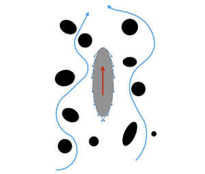
Figure 1. (a) Set-up of the problem: a spheroidal squirmer in a Brinkman medium, a viscous fluid with embedded stationary particles (represented by the black areas). The red arrow denotes the direction of swimming, while the blue arrows represent the flow of fluid through the pores (the areas filled with fluid). (b) The system of prolate spheroidal coordinates. (c) Scanning electron micrograph image of Paramecium (reproduced from Bouhouche et al. Reference Bouhouche, Valentine, Borgne, Lemullois, Yano, Lodh, Nabi, Tassin and Van Houten2022). The scale bar is 10 µm, and the red dotted curve has been added to illustrate the approximately prolate shape of the microorganism.
2.2. Governing equations
We consider a spheroidal squirmer propelling through an axisymmetric flow in an unbounded heterogeneous medium, as illustrated in figure 1(a). We begin our analysis by modelling a squirmer with constant semi-major axis length (i.e. the semi-major axis length  $a=1$ when non-dimensionalized) and circular cross-section, whose semi-minor axis length is a function of eccentricity, $e=c/a$ ( $0\leq e<1$, with $e=0$ describing a sphere). The axisymmetric incompressible flow is modelled by the Brinkman equations (1.1a,b). We non-dimensionalize lengths by a squirmer's characteristic length $L$. In §§ 3.1 and 3.2, the length scale is $L=a$, the semi-major axis length, consistent with previous studies (van Gogh et al. Reference van Gogh, Demir, Palaniappan and Pak2022). Velocities are non-dimensionalized by the first mode of actuation $B_1$, and pressure by $\mu B_1/L$. The non-dimensionalized incompressible Brinkman equations are thus given by
 \begin{equation} \nabla^2\boldsymbol{u} - \boldsymbol{\nabla} p - \delta^2\boldsymbol{u} = \boldsymbol{0},\quad \boldsymbol{\nabla}\boldsymbol{\cdot}\boldsymbol{u} = 0, \end{equation}
where the dimensionless group  $\delta = L\nu$ compares the squirmer characteristic length to the Brinkman screening length. As $\delta$ approaches zero, the Brinkman equation reduces to the Stokes equation; for large $\delta$, the equation reduces to the Darcy equation. With these scalings, the dimensionless tangential surface velocity distribution on a squirmer is given by
 \begin{equation} \boldsymbol{v}_s(\xi=\xi_0,\eta) = \xi_0 \sum^\infty_{n=1} \beta_n\,V_n(\eta)\,\boldsymbol{e}_\eta, \end{equation}
where  $\beta _n = B_n/B_1$. For a two-mode squirmer, the surface velocity reduces to $\boldsymbol {v}_s = -\xi _0(1+\beta \eta ) (1-\eta ^2)^{1/2}/(\xi _0^2-\eta ^2)^{1/2} \boldsymbol {e}_\eta$. In the frame of reference moving with the squirmer, the flow is uniform in the far field,
 \begin{equation} \boldsymbol{u}(\xi\rightarrow\infty) ={-}\boldsymbol{U}, \end{equation}
and the boundary condition on the surface of the squirmer is given by
 \begin{equation} \boldsymbol{u}(\xi=\xi_0) = \boldsymbol{v}_s. \end{equation}
To determine the propulsion velocity  $\boldsymbol {U} = U\boldsymbol {e}_z$, the system is closed by enforcing the force-free condition
 \begin{equation} \int_S\boldsymbol{n}\boldsymbol{\cdot}\boldsymbol{\sigma}\,{\rm d}S = \boldsymbol{0}, \end{equation}
where  $\boldsymbol {\sigma } = -p\boldsymbol{\mathsf{I}} + \dot {\boldsymbol {\gamma }}$ is the stress tensor expressed in terms of the identity tensor $\boldsymbol{\mathsf{I}}$ and the symmetric strain (or deformation) tensor $\dot {\boldsymbol {\gamma }} = \boldsymbol {\nabla }\boldsymbol {u} + (\boldsymbol {\nabla }\boldsymbol {u})^{\rm T}$.
2.3. Numerical simulations
We solve the governing equations using the COMSOL Multiphysics environment, building on numerical implementations from our previous studies (van Gogh et al. Reference van Gogh, Demir, Palaniappan and Pak2022; Aymen et al. Reference Aymen, Palaniappan, Demir and Nganguia2023; Della-Giustina et al. Reference Della-Giustina, Nganguia and Demir2023). To take advantage of the axial symmetry of the problem, an axisymmetric computational domain in the  $r$–
$r$– $z$ plane is used to simulate only half of the full flow domain. To simulate the locomotion of a squirmer in an unbounded fluid, we ensure that the computational domain (of size $500a \times 500b$; a and b have already been defined earlier) is sufficiently large that the numerical results are independent of the size of the domain. We achieved this by conducting convergence studies for both domain and mesh sizes. Here, $P2+P1$ (second order for fluid velocity, and first order for pressure) triangular mesh elements are used for the simulations for increased accuracy, with local mesh refinement near the squirmer to properly resolve the spatial variation of the flow field. The degree of freedom ranges from $1 \times 10^5$ to $2 \times 10^5$ for the simulations depending on eccentricity. The unknown swimming velocity of the squirmer is obtained by solving the momentum and continuity equations simultaneously with the force-free swimming condition applied on the squirmer surface. Using the parallel direct solver (PARDISO) for all simulations, we solve the fully coupled problem and obtain the velocity and pressure fields. We validated the numerical implementation against previous results for the propulsion speeds of spherical (Lighthill Reference Lighthill1952; Blake Reference Blake1971) and spheroidal (Keller & Wu Reference Keller and Wu1977; Theers et al. Reference Theers, Westphal, Gompper and Winkler2016; Pohnl et al. Reference Pohnl, Popescu and Uspal2020) squirmers in a Newtonian fluid, the power dissipation and efficiency for two-mode spheroidal squirmers in a Newtonian fluid (Appendix B). We further corroborated our numerical set-up using analytical results for spherical squirmers in heterogeneous media (Nganguia & Pak Reference Nganguia and Pak2018). For spheroidal squirmers in heterogeneous media, we developed a new analytical model that expresses the velocity field, propulsion speed, power dissipation and swimming efficiency in terms of spheroidal wave functions. Our implementation of the spheroidal wave functions, using the approach in Hodge (Reference Hodge1970) and Kirby (Reference Kirby2006), led to slow numerical convergence for large values of their argument (which in our case is given by $c \delta$). This limited the application of our analytical model to eccentricities $e\leq 0.6$, thus justifying the need for numerical simulations beyond this regime. Detailed derivations of the model are provided in Appendix C.
3. Results
The Paramecium and Oxytricha families of ciliates are examples of biological microorganisms with aspect ratios  $a/b\geq 2$, corresponding to eccentricities $e\geq 0.866$ (Rodrigues et al. Reference Rodrigues, Lisicki and Lauga2021). For this reason, in this paper we consider eccentricities up to $e=0.99$. Moreover, since the propulsion speed of a two-mode squirmer (spherical or spheroidal) in homogeneous fluids and heterogeneous media depends only on the first mode (Lighthill Reference Lighthill1952; Keller & Wu Reference Keller and Wu1977; Nganguia & Pak Reference Nganguia and Pak2018), we will focus on neutral squirmers and leave all analyses or notes regarding two-mode squirmers to the appendices. Finally, where our results are compared with the case of a spheroidal squirmer in a Newtonian fluid, the performance metrics (speed $U$, power $\mathcal {P}$ and efficiency $\zeta$) will be scaled by their corresponding values for a spheroidal squirmer in an unbounded Newtonian fluid, denoted with a subscript $N$. In a purely viscous fluid, the propulsion speed is $U_N = \xi _0[\xi _0-(\xi _0^2-1) \coth ^{-1}\xi _0]$, the power dissipation is $\mathcal {P}_N = 4{\rm \pi} c(\xi _0^2-1)[(1+\xi _0^2)\coth ^{-1}\xi _0-\xi _0]$ (where $c=1/\xi _0$), and the swimming efficiency is $\zeta _N = 2\xi _0^2[\xi _0+(1-\xi _0^2) \coth ^{-1}\xi _0]^2/(\xi _0^2-1)[\xi _0-(1+\xi _0^2) \coth ^{-1}\xi _0]^2$ (Keller & Wu Reference Keller and Wu1977; Theers et al. Reference Theers, Westphal, Gompper and Winkler2016; Pohnl et al. Reference Pohnl, Popescu and Uspal2020; van Gogh et al. Reference van Gogh, Demir, Palaniappan and Pak2022).
3.1. Propulsion speed
Figure 2(a) shows the propulsion speed  $U$ as a function of the fluid resistance $\delta$. The various curves denote different values of the eccentricity $e$, ranging from $e=0$ (spherical squirmer) to $e=0.9$ (elongated spheroidal squirmer). Increasing eccentricities yield larger speed, and we deduce that spheroidal squirmers ( $e\neq 0$) swim faster compared to spherical squirmers. In homogeneous fluids ( $\delta =0$), elongated squirmers with $e=0.9$ show upward of 15 % gain in speed compared to spherical squirmers. However, the speed decreases monotonically with increasing fluid resistance. We can also contrast the propulsion of a spheroidal squirmer in homogeneous vs heterogeneous media. As illustrated in figure 2(b), a squirmer in a heterogeneous medium always swims slower compared to a squirmer in a homogeneous fluid. However, while the squirmer experiences a reduction in speed, more elongated squirmers are able to maintain speeds close to that of their counterpart in Newtonian fluids for a wider range of fluid resistance. Indeed, significant reduction in speed becomes more visible around $\delta =1$ for $e<0.6$ and around $\delta \approx 4$ for $e=0.9$.

Figure 2. Propulsion speed as a function of the fluid resistance  $\delta$ for different values of eccentricity. In (b), the speed is scaled by its corresponding value for a spheroidal squirmer in a Newtonian fluid: $U_N = \xi _0[\xi _0-(\xi _0^2-1) \coth ^{-1}\xi _0]$. In both plots, the symbols denote numerical simulations using the finite element method (FEM), while the dashed, solid and dotted lines denote prediction for spherical ( $e=0$) and spheroidal ( $e=0.3,0.6$) neutral squirmers using the analytical models for spherical squirmers in Nganguia & Pak (Reference Nganguia and Pak2018) and the proposed model for spheroidal squirmers developed in Appendix C.
These observations can be made more clearly by plotting the speed as a function of the eccentricity for various values of the fluid resistance. As seen in figure 3(b), increasing the fluid resistance yields a decrease in the propulsion speed for a fixed eccentricity, while increasing eccentricity yields to faster swimmers for a fixed fluid resistance. Figure 3(a) shows the propulsion speed scaled by the speed of a spherical squirmer in the same fluid environment, and suggests that spheroidal squirmers swim faster compared to spherical squirmers. The figure also demonstrates that the effects of shape become even more pronounced in highly heterogeneous media: a very elongated squirmer ( $e\approx 0.99$) that experiences high fluid resistance ( $\delta =100$) sees a greater than ten-fold increase in speed over a spherical squirmer in homogeneous or heterogeneous media, and a nearly 10 % increase in speed over a similarly shaped squirmer in a homogeneous fluid. Another interesting result arises from analysing the speed scaled by the speed $U_{NS}$ of a spherical squirmer in a homogeneous fluid (Lighthill Reference Lighthill1952). In this case, figure 3(b) shows that spheroidal squirmers in heterogeneous media can propel faster compared to spherical squirmers in homogeneous fluids. The critical eccentricity at which this trend occurs is represented by the dashed curve in figure 3(c).

Figure 3. Propulsion speed as a function of the eccentricity  $e$ for different values of the fluid resistance $\delta$. Lines indicate analytical results, and symbols indicate numerical results. (a) The speed of the spheroidal squirmer in the Brinkman medium is scaled by the speed of the spherical squirmer in the same environment (with the same $\delta$). (b) The speed is scaled by its corresponding value $U_{NS}=2/3$ for a spherical squirmer ( $e=0$) in a Newtonian fluid ( $\delta =0$). (c) The $\delta \unicode{x2013}e$ diagram delimitates the regions where enhanced ( $U/U_{NS}>1$) and hindered ( $U/U_{NS}<1$) swimming occur. The dashed line indicates $U/U_{NS}=1$.
A good indication of the effect that a micro-swimmer has on its surroundings and/or on hydrodynamic interactions is how fast its flow decays. For a spherical neutral squirmer, the flow decays as  ${\sim }1/r^3$ in homogeneous and heterogeneous media (Nganguia & Pak Reference Nganguia and Pak2018). Figure 4 shows the component of velocity $w$ in the swimming direction as a function of the distance from the squirmer's semi-major axis $a$. Figures 4(a,b) show variations in $w$ that result from changes in the eccentricity for a fixed fluid resistance $\delta =0$ and $100$, respectively. The velocity component on the surface of a spheroidal squirmer is larger than that on the surface of a spherical squirmer. However, this difference shows a strong dependence on the fluid resistance: it is insignificant in a homogeneous fluid, and becomes more evident in a heterogeneous medium. Away from the micro-swimmer, the flow near the squirmer decreases significantly with increasing eccentricity in homogeneous fluids, while it becomes independent of shape in highly heterogeneous media. Summarizing figures 4(a,b), the difference in the flow between spheroidal and spherical squirmers depends on the near or far field: spheroidal squirmers experience greater flow than that of spherical squirmers at close proximity with the micro-swimmers. On the other end, in the far field, the flow becomes independent of the micro-swimmers’ shape. When we fix $e=0.6$ instead, and vary the fluid resistance (figure 4c), we observe that the flow decreases significantly with increasing fluid resistance. This trend is consistent with the results in figure 2 that show the propulsion speed decreasing monotonically with increasing fluid resistance. Finally, one common feature in figure 4 is that the flow decays as ${\sim }1/r^3$ independently of $e$ and $\delta$, and consistent with the flow decay for spherical neutral squirmers.

Figure 4. Velocity component in the swimming direction as a function of the distance from the surface of the spheroidal squirmer. (a,b) Effect of eccentricity on velocity for (a)  $\delta = 0$ and (b) $\delta = 100$. (c) Effect of heterogeneity on velocity for $e=0.6$. The black dash-dotted line is added to represent the slope ${\sim }1/r^3$ in the far field. Note that the flow is plotted in the laboratory frame where $\boldsymbol {u}\rightarrow \boldsymbol {0}$ as $r\rightarrow \infty$.
3.2. Power dissipation and swimming efficiency
A spherical squirmer in a heterogeneous medium expends more energy to swim as the fluid resistance increases. Although power dissipation increases monotonically with fluid resistance, Nganguia & Pak (Reference Nganguia and Pak2018) reported that under these conditions, the squirmer actually swims more efficiently for low to moderate values of the fluid resistance.
In this subsection, we discuss the power dissipation and swimming efficiency for a spheroidal squirmer propelling in a heterogeneous medium. The power dissipation is calculated using
 \begin{equation} \mathcal{P} ={-}\int_S\boldsymbol{n}\boldsymbol{\cdot}\boldsymbol{\sigma}\boldsymbol{\cdot}\boldsymbol{u}\,{\rm d}S, \end{equation}
while the swimming efficiency is obtained using Lighthill's definition (Lighthill Reference Lighthill1952) of the ratio of the power required to tow a rigid spheroid in uniform motion with velocity  $U$ to the work done by the squirmer:
 \begin{equation} \zeta = \frac{\mathcal{P}_D}{\mathcal{P}} = \frac{\boldsymbol{F_D}\boldsymbol{\cdot}\boldsymbol{U}}{\mathcal{P}}, \end{equation}
where  $\boldsymbol {F}_D$ is the drag force. Intuitively, one may expect the power dissipation of spheroidal squirmers to decrease with increasing eccentricity, the elongated shape of the squirmer making it easier to navigate around the stationary obstacles. This is certainly captured in figure 5(a). We also note that the largest influence of shape is observed in highly heterogeneous media, where the difference in power dissipation between spherical squirmers ( $\mathcal {P}=800$) and elongated squirmers with, for example, $e=0.9$, stands at 300 (a 62.5 % reduction).

Figure 5. Power dissipation as a function of the fluid resistance  $\delta$ for different values of eccentricity. In (b), the power is scaled by its corresponding value for a spheroidal squirmer in a Newtonian fluid: $\mathcal {P}_N = 4{\rm \pi} c(\xi _0^2-1)[(1+\xi _0^2)\coth ^{-1}\xi _0-\xi _0]$ or (B12) with $\beta _2=0$. (c) Power dissipation as a function of eccentricity $e$ for different values of the fluid resistance. The variable is scaled by its corresponding values for a spherical squirmer ( $e=0$).
When the power dissipation in a heterogeneous medium is scaled by that in a homogeneous fluid, one immediately observes that spheroidal squirmers in heterogeneous media expend more energy compared to their counterparts in homogeneous fluids. However, a number of intriguing behaviours emerge. For  $e\leq 0.6$, the curves collapse together up to approximately $\delta =50$, when squirmers with higher eccentricity have higher power dissipation as the fluid resistance continues to increase. Moreover, squirmers with $e=0.9$ can yield either lower or higher power dissipation compared to less elongated squirmers. The outcome depends on specific combinations of the eccentricity and medium's resistance: for example, for $\delta <60$ ( $\delta >60$), squirmers with $e=0.9$ exert less (more) power dissipation compared to squirmers with $e\leq 0.3$. Unlike the propulsion speed and the power dissipation, the swimming efficiency displays a non-monotonic behaviour as a function of the fluid resistance. As the latter increases, the efficiency reaches a maximum before converging to zero at high values of the fluid resistance. Figure 6(a) shows that greater efficiency can be achieved by replacing spherical with spheroidal squirmers. Furthermore, we found that spheroidal squirmers in heterogeneous media are more efficient compared to their counterparts in homogeneous fluids for low to moderate $\delta$, as illustrated in figure 6(b). This is consistent with the efficiency of a spherical squirmer (Nganguia & Pak Reference Nganguia and Pak2018). We further observe that squirmers with $e\leq 0.6$ yield nearly identical efficiencies over the range of fluid resistance.

Figure 6. Swimming efficiency as a function of the fluid resistance  $\delta$ for different values of eccentricity, using FEM and prolate spheroidal wave functions (PSWF) (dashed curves in (a) and (b)). In (b), the efficiency is scaled by its corresponding value for a spheroidal squirmer in a Newtonian fluid: $\zeta _N = 2\xi _0^2[\xi _0+(1-\xi _0^2)\coth ^{-1}\xi _0]^2/(\xi _0^2-1)[\xi _0-(1+\xi _0^2) \coth ^{-1}\xi _0]^2$ or (B15) with $\beta _2=0$. (c) Swimming efficiency as a function of eccentricity $e$ for different values of the fluid resistance. The variable is scaled by its corresponding values for a spherical squirmer ( $e=0$).
Note that for sufficiently slender-shaped ( $e>0.8$) tangential squirmers in homogeneous fluid, the power dissipation is $\mathcal {P}<\mathcal {P}_D$ (Keller & Wu Reference Keller and Wu1977). This observation justifies the curve with $\zeta >1$ ( $e=0.9$) at low to moderate $\delta$ values in figure 6(a). However, using the spheroidal squirmer model (1) yields the power dissipation only outside the ciliary envelope (the layer representing the boundary of beating cilia), and (2) omits interactions of the individual cilia with the surrounding medium. Considering a ciliate model to mimic microorganisms such as Tetrahymena, Ito, Omori & Ishikawa (Reference Ito, Omori and Ishikawa2019) reported that the power dissipation generated within the ciliary envelope can contribute as high as $\sim$90 % of the total power dissipation from both inside and outside the envelope. Therefore, since much of the power is generated within the ciliary envelope, efficiencies $\zeta >1$ are plausible only for cilia much shorter than the cell body length scale $L$ and the damping length scale $\alpha ^{-1}$.
Plotting the power dissipation (figure 5c) and swimming efficiency (figure 6c) as a function of the squirmer's eccentricity enables us to better compare the effects of heterogeneity and shape on spherical versus spheroidal squirmers. In both figures, the variables are scaled by the corresponding values for a spherical squirmer. As a general trend, for a fixed value of the fluid resistance, spheroidal squirmers expend less energy and are more efficient swimmers compared to spherical squirmers in both homogeneous and heterogeneous media. However, we observe two distinct regimes across the range of fluid resistance. As illustrated in figure 5(c), the power dissipation is non-monotonic: it first decreases as  $\delta$ approaches 10, then increases for $\delta \gg 10$. Figure 6(c) shows a similar non-monotonic trend for the swimming efficiency, albeit this behaviour occurs at a value of the fluid resistance an order of magnitude smaller ( $\delta \approx 1$).
3.3. Biological modelling
The results in the previous analysis have been obtained for general spheroidal microorganisms without constraints on surface area or volume, instead considering constant semi-major length  $L=a$ (van Gogh et al. Reference van Gogh, Demir, Palaniappan and Pak2022). Rodrigues et al. (Reference Rodrigues, Lisicki and Lauga2021) showed that the corresponding propulsion speed $U_N = \xi _0[\xi _0-(\xi _0^2-1) \coth ^{-1}\xi _0]$ agreed with the experimentally measured range of velocities experienced by ciliates from different taxonomic classes. While solutions obtained using $a$ to scale the problem have yielded good agreement with experimental data, our formulation can also be adapted to account for other geometrical and biologically relevant constraints. For example, under the assumption of fixed volume ( $L=V^{1/3}$, where $V$ is the volume of the squirmer), the spheroidal squirmer must satisfy $ab^2\approx r_0^3$, where $r_0$ is the radius of a spherical squirmer with the same volume as the spheroidal squirmer. Generally, the shape parameter is given by $\xi _0=a/c$. Under constant volume of the squirmer, we determine $a=(4{\rm \pi} /3)^{-1/3}(1-1/\xi _0^2)^{-1/3}$, $b=(4{\rm \pi} /3)^{-1/3}(1-1/\xi _0^2)^{1/6}$ and $c=(4{\rm \pi} /3)^{-1/3}(\xi _0^3-\xi _0)^{-1/3}$. In other words, the lengths that define the spheroidal shape of the organisms now vary with eccentricity through $\xi _0$.
Our simulations show that the volume constraint does not alter the qualitative results that we obtained under the assumption of constant semi-major length. This is illustrated in figure 7, where the propulsion speed, power dissipation and swimming efficiency of squirmers with different aspect ratios but equal volume are scaled by corresponding values in Newtonian fluids. All variables are plotted as functions of the fluid resistance. As observed in figures 7(a,c), squirmers of equal volume and eccentricity  $e<0.9$ propel at the same speed and swimming efficiency, whereas very elongated squirmers ( $e\geq 0.9$) benefit from small but noticeable gains in both speed and efficiency. The effect of eccentricity with fixed volume is more pronounced in terms of the power dissipation (figure 7b), where we observe that the latter increases consistently with both eccentricity and fluid resistance. This contrasts with the power dissipation with fixed semi-major length (figure 5b), where the power dissipation increased with fluid resistance but exhibited a non-trivial behaviour as a function of eccentricity.

Figure 7. (a) Swimming velocity, (b) power dissipation, and (c) efficiency normalized by their corresponding Newtonian values ( $\delta =0$) for the spheroidal squirmers with the constant-volume constraint. Excellent qualitative agreement with the constant semi-major length analysis (figures 2, 5(b), and 6(b), respectively) is observed.
3.4. Force analysis
In this subsection, we discuss changes in the forces that act to generate propulsion of the squirmer and how they vary with eccentricity ( $e$) and fluid resistance ( $\delta$).
We decompose the force-free condition into
 \begin{equation} \int_S \boldsymbol{\sigma}\boldsymbol{\cdot}\boldsymbol{n}\,{\rm d}S = \underbrace{\int_S ({-}p)\textbf{I}\boldsymbol{\cdot}\boldsymbol{n}\,{\rm d}S }_{\boldsymbol{F}_{pres}} + \underbrace{\int_S \dot{\boldsymbol{\gamma}}\boldsymbol{\cdot}\boldsymbol{n}\,{\rm d}S }_{\boldsymbol{F}_{visc}} = \boldsymbol{0}, \end{equation}
where  $\boldsymbol {F}_{pres}$ is the contribution due to pressure, and $\boldsymbol {F}_{visc}$ results from the viscous stress. In the swimming direction, our numerical simulations confirm that these two forces are equal in magnitude with opposite signs.
Figure 8 illustrates the variation of the viscous (figures 8a,c) and pressure (figures 8b,d) forces as a function of the eccentricity for different values of the fluid resistance. Each force is further decomposed into contributions that result from the towing and pumping dynamics. Specifically, the results represent the forces exerted by the surrounding medium on the squirmer. Both the viscous and pressure forces reveal a strong dependence on the eccentricity and the fluid resistance. We can rewrite the decomposition in (3.3) as
 \begin{equation} \boldsymbol F_{pump}+\boldsymbol F_{tow} = \boldsymbol{0}, \end{equation}
where  $\boldsymbol F_{pump}$ is the pumping force generated by the squirmer when it is being held fixed, while $\boldsymbol F_{tow} = \alpha (\delta )\,\boldsymbol {U}$ is the force required to tow the squirmer at a given velocity $\boldsymbol {U}$. In this last expression, $\alpha (\delta )$ is the translational drag coefficient (Yang et al. Reference Yang, Lu, Zhao and Kawamura2017) that, in our analysis, also depends on the fluid resistance. From this, we express the propulsion speed as
 \begin{equation} \boldsymbol{U} ={-} \frac{\boldsymbol{F}_{pump}}{\alpha(\delta)}. \end{equation}
This relation, along with the results in figure 9, provides justification for the behaviour observed in figures 2 and 7(a): the propulsion speed decreases with increasing fluid resistance. Indeed, when the semi-major axis length is constant (figure 9a), the pumping force (right-hand axis in the figure, denoted by lines) decreases (increases) with increasing eccentricity (fluid resistance). The same trend is observed for the drag coefficient (left-hand axis in the figure, denoted by symbols). In the case of constant volume (figure 9b), the pumping force increases with both eccentricity and fluid resistance. The drag coefficient also increases with higher fluid resistance, but shows a non-monotonic trend as a function of eccentricity:  $\alpha$ generally decreases with increasing eccentricity, except for $e\gg 0.9$. In both cases, the magnitude of the drag coefficient is higher compared with the pumping force ( $|\alpha (\delta )|\geq |\boldsymbol {F}_{pump}|$). Ultimately, this leads to a slower propulsion speed as the fluid resistance increases.

Figure 8. (a,c) Viscous stress contribution, and (b,d) pressure contribution to the force in the swimming direction  $z$ as function of the eccentricity. (a,b) Results for the constant semi-major axis length ( $e=c$); (c,d) results for the constant-volume cases. In all plots, the curves denote different values of the fluid resistance with ${\delta =0,1,5,10}$, lines depict the pumping forces, and symbols depict the towing forces.

Figure 9. Translational drag coefficient (symbols, left-hand axis) and magnitude of the pumping force (lines, right-hand axis) as functions of eccentricity for (a) constant semi-major length and (b) constant-volume constraints.
4. Concluding remarks
The spheroidal geometry encompasses spheres, cylinders and disks in their respective limits. This versatility makes the spheroidal squirmer model ideal to investigate the effects of shape on the propulsion of non-spherical micro-swimmers. Expanding upon work by Nganguia & Pak (Reference Nganguia and Pak2018) on spherical squirmers, we investigate numerically how the micro-swimmer's geometry impacts locomotion in heterogeneous viscous media.
Our results show that spheroidal squirmers in heterogeneous media experience reduced speed, increased energy expenditure and enhanced swimming efficiency compared to their counterparts in homogeneous fluids. This is not unlike the case of spherical squirmers (Nganguia & Pak Reference Nganguia and Pak2018). However, spheroidal squirmers in heterogeneous media display superior swimming performance over spherical squirmers. Specifically, we found that heterogeneous media present the ideal swimming environment, with enhancement in propulsion speed and efficiency, and a reduction in energy cost. Indeed, spheroidal squirmers in heterogeneous media can swim faster (figure 3c), expend less energy (up to  $\delta \leq 10$; figure 5c) and swim as or more efficiently (up to $\delta \geq 100$; figure 6c) compared with spherical squirmers in homogeneous fluids.
We also examine how the pressure and viscous forces vary as functions of both the eccentricity and fluid resistance. Remarkably, we found that while the selection of geometrical constraints had no impact on the qualitative behaviour of the kinematic and energetic factors, it showed more pronounced effects on the forces. Based on these findings, we were able to explain why the propulsion speed decreases in a heterogeneous medium.
Recent studies have investigated the propulsion of spheroidal microorganisms in microchannels (Theers et al. Reference Theers, Westphal, Gompper and Winkler2016; Qi et al. Reference Qi, Annepu, Gompper and Winkler2020) and in environments described by Newtonian (Theers et al. Reference Theers, Westphal, Gompper and Winkler2016; Pohnl et al. Reference Pohnl, Popescu and Uspal2020) and complex (van Gogh et al. Reference van Gogh, Demir, Palaniappan and Pak2022) fluids. Our findings complement these studies related to spheroidal microorganisms by addressing swimming in heterogeneous media. Interesting subjects for future studies include the ways in which our findings will influence the hydrodynamic interaction of swimmers as well as nutrient transport and uptake by microorganisms in heterogeneous viscous environments. Work in these directions is currently under way.
Funding
H.N. gratefully acknowledges funding support from the National Science Foundation grant no. 2211633, and from a Jess and Mildred Fisher Endowed Professor of Mathematics from the Fisher College of Science and Mathematics at Towson University.
Declaration of interests
The authors report no conflict of interest.
Appendix A. Prolate spheroidal coordinate system
Recall the prolate spheroidal coordinate system given by  $(\xi,\eta,\phi )$, where $1\leq \xi <\infty$, $-1\leq \eta \leq 1$ and $0\leq \phi \leq 2{\rm \pi}$ (figure 1b). The position vector of the squirmer in cylindrical coordinates is given by
 \begin{equation} \boldsymbol{x} = c\,\sqrt{\xi^2-1}\,\sqrt{1-\eta^2}\,\boldsymbol{e}_r + c\xi\eta\,\boldsymbol{e}_z, \end{equation}
where the basis vectors satisfy  $\boldsymbol {e}_r=\cos \phi \,\boldsymbol {e}_x+\sin \phi \,\boldsymbol {e}_y$, and $c=\sqrt {a^2-b^2}$ is the semi-focal length of the spheroid, with $a=c\xi$ and $b=c\sqrt {\xi ^2-1}$. The eccentricity of the squirmer is $e=c/a$, and we define the shape parameter $\xi _0=1/e$, where $\xi >\xi _0$ denotes the fluid domain excluding the surface ( $\xi = \xi _0$). In this coordinate system, the metric coefficients are given by
 \begin{equation} h_\xi = c\,\sqrt{\frac{\xi^2-\eta^2}{\xi^2-1}},\quad h_\eta = c\,\sqrt{\frac{\xi^2-\eta^2}{1-\eta^2}},\quad h_\phi = c\,\sqrt{(\xi^2-1)(1-\eta^2)}, \end{equation}
and the unit basis vectors are related to those in the Cartesian coordinates by
 \begin{equation} \boldsymbol{e}_\xi = \frac{\xi\sqrt{1-\eta^2}}{\sqrt{\xi^2-\eta^2}}\,\boldsymbol{e}_r + \frac{\eta\sqrt{\xi^2-1}}{\sqrt{\xi^2-\eta^2}}\,\boldsymbol{e}_z,\quad \boldsymbol{e}_\eta ={-}\frac{\eta\sqrt{\xi^2-1}}{\sqrt{\xi^2-\eta^2}}\,\boldsymbol{e}_r + \frac{\xi\sqrt{1-\eta^2}}{\sqrt{\xi^2-\eta^2}}\,\boldsymbol{e}_z. \end{equation}
Appendix B. Outline of the derivation for the power dissipation and swimming efficiency of a two-mode squirmer in a Newtonian fluid
Motivated by the approximately prolate spheroidal bodies of many ciliates, we use the prolate spheroidal coordinates  $(\xi,\eta,\phi )$ to derive a series solution for the propulsion speed of a prolate microorganism. The power dissipation and swimming efficiency of a spheroidal squirmer have also been reported, but only for a neutral squirmer (Keller & Wu Reference Keller and Wu1977). To fill this gap in knowledge and complement existing studies, here we derive analytical expressions for the power dissipation and swimming efficiency for a two-mode squirmer.
The derivations follow similar approaches used for the neutral squirmer (Keller & Wu Reference Keller and Wu1977; van Gogh et al. Reference van Gogh, Demir, Palaniappan and Pak2022).
We consider an axisymmetric flow, and express the flow field in terms of the stream function  $\psi _N$ as (Dassios Reference Dassios2007)
 \begin{equation} \boldsymbol{u}_N = u_N\boldsymbol{e}_\xi + v_N\boldsymbol{e}_\eta = \frac{1}{h_\eta h_\phi}\,\frac{\partial\psi_N}{\partial\eta}\,\boldsymbol{e}_\xi - \frac{1}{h_\xi h_\phi}\,\frac{\partial\psi_N}{\partial\xi}\,\boldsymbol{e}_\eta, \end{equation}
where
 \begin{equation} \psi_N = C_1\,H_2(\xi)\,G_2(\eta) + C_2\xi(1-\eta^2) + C_3\,H_3(\xi)\,G_3(\eta) +C_4\eta(1 - \eta^2), \end{equation}
where the coefficients  $C_i$ are easily obtained after applying the boundary conditions, and the functions $G_n(x)$ and $H_n(x)$ are the Gegenbauer functions of the first and second kind, respectively, given by (Dassios, Hadjinicolaou & Payatakes Reference Dassios, Hadjinicolaou and Payatakes1994)
 \begin{equation} \left.\begin{gathered} G_2(x) = \frac{1}{2}\,(1-x^2), \\ G_3(x) = \frac{1}{2}\,(x-x^3), \\ H_2(x) = \frac{1}{4}\,(1-x^2)\ln\left(\frac{x+1}{x-1}\right) + \frac{x}{2}, \\ H_3(x) = \frac{1}{12}\left[{-}4+6x^2+3x(x^2-1)\ln\left(\frac{x-1}{x+1}\right) \right]. \end{gathered}\right\} \end{equation}
It can be shown that the pressure is given by
 \begin{equation} p_N = \frac{-2(C_2\eta+3C_4\xi) + 6C_4(\xi^2-\eta^2)\coth^{{-}1}\xi}{c^3(\xi^2-\eta^2)}. \end{equation}
The total force on the spheroidal squirmer in the direction of motion is given by
 \begin{equation} F = 2{\rm \pi} c^2\sqrt{\xi_0^2-1} \int^1_{{-}1} \left[({-}p_N+\dot{\boldsymbol{\gamma}}_{\xi\xi})|_{\xi_0}\,\eta\sqrt{\xi_0^2-1} + \dot{\boldsymbol{\gamma}}_{\eta\xi}|_{\xi_0}\,\xi_0\sqrt{1-\eta^2}\right]{\rm d}\eta, \end{equation}
which reduces to
 \begin{equation} F = \left(\int_S \boldsymbol{\sigma}\boldsymbol{\cdot}\boldsymbol{n}\,{\rm d}S\right)\boldsymbol{\cdot} \boldsymbol{e}_z = \frac{8{\rm \pi} C_2}{c}. \end{equation}
 The swimming problem can be decomposed into two sub-problems: a towing problem ( $T$) and a pumping problem ( $P$) (Pak & Lauga Reference Pak and Lauga2014; Nganguia & Pak Reference Nganguia and Pak2018). The force resulting from each problem is given by (B6), with the coefficient $C_2$ determined from boundary conditions for the specific problem. The force-free condition for the propulsion of a spheroidal squirmer in a Newtonian fluid, $\bigl (\int _S \boldsymbol {\sigma }\boldsymbol {\cdot }\boldsymbol {n}\,\textrm {d}S\bigr )\boldsymbol {\cdot }\boldsymbol {e}_z = F_P + F_T = 0$, reduces to
 \begin{equation} C_2^T + C_2^P = 0, \end{equation}
where
 \begin{equation} C_2^T = \frac{U c^2}{2}\,\frac{(\xi_0^2-1)\,H_2'(\xi_0) - 2\xi_0\,H_2(\xi_0)}{H_2(\xi_0) - \xi_0\,H_2'(\xi_0)} \end{equation}
and
 \begin{equation} C_2^P = \frac{\xi_0 c^2\,H_2(\xi_0)}{H_2(\xi_0) - \xi_0\,H_2'(\xi_0)} \end{equation}
are the coefficients corresponding to the towing and pumping problems, respectively. Substituting the coefficients, solving for the propulsion speed, and simplifying using the definition for the inverse hyperbolic cotangent  $\ln [(x+1)/(x-1)]/2 = \coth ^{-1}x$, yields
 \begin{equation} U_N = \xi_0[\xi_0-(\xi_0^2-1) \coth^{{-}1}\xi_0]. \end{equation}
Once the flow field is determined, the power dissipation  $\mathcal {P}_N = - \int _S\boldsymbol {n}\boldsymbol {\cdot }\boldsymbol {\sigma }\boldsymbol {\cdot }\boldsymbol {u}_N\,\textrm {d}S$ can be calculated. In spheroidal coordinates,
 \begin{equation} \mathcal{P}_N = 2{\rm \pi} c^2 \int^{1}_{{-}1} (u_N \sigma_{\xi\xi} + v_N \sigma_{\xi\eta})|_{\xi_0}\, \sqrt{(\xi_0^2-1)(\xi_0^2-\eta^2)}\,{\rm d}\eta, \end{equation}
and after lengthy calculations, one can show that
 \begin{equation} \mathcal{P}_{N} = \mathcal{P}_{B_1}+ \mathcal{P}_{B_2}, \end{equation}
where
 \begin{equation} \left.\begin{gathered} \mathcal{P}_{B_1} ={-}4{\rm \pi} c(\xi_0^2-1)[\xi_0-(\xi_0^2+1)\coth^{{-}1}{\xi_0}], \\ \mathcal{P}_{B_2} ={-}\frac{4{\rm \pi} c \xi_0^2 \beta^2}{9\xi_0-(9\xi_0^2-3)\coth^{{-}1}{\xi_0}}\, \{8-51 \xi_0^2+45\xi_0^4 \\ \quad {}+3(\xi_0^2-1)\coth^{{-}1}{\xi_0}\, [14\xi_0-30\xi_0^3+(1-12\xi_0^2+15\xi_0^4)\coth^{{-}1}{\xi_0}]\}. \end{gathered}\right\} \end{equation}
We then use the power dissipation to calculate the swimming efficiency (Lighthill Reference Lighthill1952):
 \begin{equation} \zeta_N = \frac{\boldsymbol{F}_D\boldsymbol{\cdot}\boldsymbol{U}_N}{\mathcal{P}_N}, \end{equation}
where  $\boldsymbol {F}_D$ is the drag force for a spheroidal squirmer in a homogeneous fluid, or the force needed to pull a rigid spheroid at the swimming velocity $\boldsymbol {U}_N=U_N\boldsymbol {e}_z$. We find that the swimming efficiency is given by
 \begin{equation} \zeta_{N} = \frac{6\xi_0^2[\xi_0-(\xi_0^2-1)\coth^{{-}1} \xi_0]^2\,[3 \xi_0-(3\xi_0^2-1) \coth^{{-}1} \xi_0]}{H_1 +\beta^2H_2}, \end{equation}
where
 \begin{equation} \left.\begin{gathered} H_1 = 3(\xi_0^2-1)[\xi_0-(\xi_0^2+1)\coth^{{-}1} \xi_0]^2\, [3\xi_0- (3\xi_0^2-1)\coth^{{-}1} \xi_0], \\ H_2 = \xi_0^2 [\xi_0-(\xi_0^2+1)\coth^{{-}1} \xi_0] \{8-51 \xi_0^2+45\xi_0^4+3(\xi_0^2-1)\coth^{{-}1}{\xi_0} \\ \quad {}\times [14\xi_0-30\xi_0^3+(1-12\xi_0^2+15\xi_0^4)\coth^{{-}1}{\xi_0}]\} \end{gathered}\right\}. \end{equation}
To validate these expressions, we compare them against numerical results for the case  $\delta =0$ (Newtonian fluids). Figures 10(a,b) show excellent quantitative agreement between the analytical results and the numerical simulations for the power dissipation and swimming efficiency of a neutral squirmer and a pusher with $\beta =1$. The results in figure 10(a) show that more elongated, spheroidal squirmers expend less energy in swimming compared to spherical squirmers. In terms of swimming efficiency, figure 10(b) shows that spheroidal squirmers are more efficient compared with spherical squirmers. Note that for a two-mode squirmer, the propulsion speed still depends on the first mode alone. More generally, only the odd modes contribute to the propulsion speed (Pohnl et al. Reference Pohnl, Popescu and Uspal2020). This also suggests that, unlike the case for a spherical squirmer, a spheroidal squirmer can locomote in the absence of the first mode, propelled by the $B_{2n+1}$ modes.

Figure 10. (a) Power dissipation and (b) swimming efficiency for a spheroidal squirmer as a function of the eccentricity  $e$. Both variables are scaled by the corresponding values for a spherical squirmer ( $e=0$), and the fluid is Newtonian ( $\delta =0$). Curves are obtained from (B12) and (B15), while the symbols denote numerical simulations. The curves are colour-coded to represent a neutral squirmer (black) and puller (blue).
Appendix C. Analytical solution for the propulsion of a spheroidal squirmer in a Brinkman medium and validation of the numerical implementation
In this appendix, we derive the propulsion speed, power dissipation and swimming efficiency for a prolate spheroidal squirmer in a Brinkman medium. While semi-separable solutions in spheroidal coordinates (Dassios et al. Reference Dassios, Hadjinicolaou and Payatakes1994) can be utilized for harmonic and biharmonic equations, the case for Brinkman flows requires solutions of the Helmholtz equations. It is known that solutions of the Helmholtz equations can be written in terms of series of the so-called spheroidal wave functions (Aoi Reference Aoi1955; Stratton et al. Reference Stratton, Morse, Chu, Little and Corbato1956; Flammer Reference Flammer1957; Abromowitz & Stegun Reference Abromowitz and Stegun1964). These mathematically sophisticated special functions have been employed mainly in the context of electromagnetic or sound wave propagation. For instance, they have been used to derive electrophoretic mobility functions of spheroidal particles (Yoon & Kim Reference Yoon and Kim1989; Miloh & Goldstein Reference Miloh and Goldstein2015). The model that we developed becomes slow-converging with increasing eccentricity, and performs best for eccentricity up to 0.6, thus justifying our use of numerical simulations to investigate shape effects with  $e>0.6$.
We again assume axial symmetry and express the Brinkman equation in terms of a stream function  $\varPsi$. Substituting (B1) into the Brinkman equation (2.2a,b) gives
 \begin{equation} D^2(D^2 - \delta^2 )\varPsi = 0, \end{equation}
where
 \begin{equation} D^2 = \frac{1}{c^2(\xi^2-\eta^2)} \left[(\xi^2 -1)\,\frac{\partial^2}{\partial \xi^2} + (1-\eta^2)\,\frac{\partial^2}{\partial \eta^2}\right]. \end{equation}
 Equation (C1) can be solved by letting  $\varPsi = \varPsi ^{(1)} + \varPsi ^{(2)}$, where $\varPsi ^{(1)}$ satisfies ${D^2\varPsi ^{(1)} = 0}$, and $\varPsi ^{(2)}$ satisfies $(D^2-\delta ^2) \varPsi ^{(2)} = 0$. The general solutions are
 \begin{align} \varPsi^{(1)} &= \sqrt{(\xi^2-1)(1-\eta^2)} \sum_{n = 1}^{\infty} C_{n}^1\,P^1_n(\xi)\,P^1_n(\eta) + C_{n}^2\,P^1_n(\xi)\,Q^1_n(\eta) \nonumber\\ &\quad +C_{n}^3\,Q^1_n(\xi)\,Q^1_n(\eta) + C_{n}^4\,Q^1_n(\xi)\,P^1_n(\eta) \end{align}
and
 \begin{align} \varPsi^{(2)} &= \sqrt{(\xi^2-1)(1-\eta^2)} \sum_{k = 1}^{4} \sum_{n = 1}^{\infty} E^{k}_n\,R^{(k)}_{1n}({\rm i}\chi,\xi)\,S^{(1)}_{1n}({\rm i}\chi,\eta) \nonumber\\ &\quad +E^{k+4}_n\,R^{(k)}_{1n}({\rm i}\chi,\xi)\,S^{(2)}_{1n}({\rm i}\chi,\eta), \end{align}
where  $\chi =\delta c$, $P_{n}^m(x)$ and $Q_{n}^m(x)$ are associated Legendre functions of the first and second kind of order $m$ and degree $n$, respectively, and $R^{(k)}_{1n}$ and $S^{(j)}_{1n}$ are radial and angular wave functions, respectively. The superscripts $k=1,2,3,4$ and $j=1,2$ are the orders of the prolate wave functions. Each of the four radial prolate wave functions is related to spherical Bessel functions $j_n,y_n,h_n^{(1)}$ and $h_n^{(2)}$, while the angular wave functions each correspond to associated Legendre functions.
The constants  $C_n$ and $E_n$ in the general solutions (C3) and (C4) are determined from applying boundary conditions. Specifically, since the flow field is bounded in the domain $\xi _0\leq \xi <\infty$ and $-1\leq \eta \leq 1$, we must have $C_{n}^1 = C_{n}^2 = C_{n}^3 = 0$, and $\varPsi ^{(1)}$ reduces to
 \begin{equation} \varPsi^{(1)} = \sqrt{(\xi^2-1)(1-\eta^2)} \sum_{n = 1}^{\infty} C_{n}\,Q^1_n(\xi)\,P^1_n(\eta). \end{equation}
Regarding  $\varPsi ^{(2)}$, the angular functions satisfy $S^{(2)}_{1n}(\textrm {i}\chi,\eta )\rightarrow \infty$, whereas only the radial functions of the third kind ( $k=3$) decay exponentially as $\xi \rightarrow \infty$, so we must have $E^{k+4}_n = 0$ and $E^{1}_n = E^{2}_n = E^{4}_n = 0$. The stream function reduces to
 \begin{equation} \varPsi^{(2)} = \sqrt{(\xi^2-1)(1-\eta^2)} \sum_{k = 1}^{4} \sum_{n = 1}^{\infty} E_n\,R^{(3)}_{1n}({\rm i}\chi,\xi)\,S^{(1)}_{1n}({\rm i}\chi,\eta), \end{equation}
where
 \begin{equation} \left.\begin{gathered} R^{(3)}_{1n}({\rm i}\chi,\xi) = \left[{\rm i}^{n+2} \sum_{r=0,1}^{\infty}{}^{'} (r+1)(r+2)\,d_r^{1n}({\rm i}\chi) \right]^{{-}1} \\ \quad {}\times \sqrt{\frac{2}{{\rm \pi}\chi}}\,\sqrt{\frac{\xi^2-1}{\xi^3}} \sum_{r=0,1}^{\infty}{}^{'} (r+1)(r+2)\,d_r^{1n}({\rm i}\chi)\,K_{r+{3}/{2}}(\chi\xi), \\ S^{(1)}_{1n}({\rm i}\chi,\eta) = \sum_{r=0,1}^{\infty}{}^{'} d_r^{1n}({\rm i}\chi)\,P_{r+1}^1(\eta) \end{gathered}\right\} \end{equation}
and  $K_{r+{3}/{2}}(\chi \xi )$ are the modified Bessel functions. The prime indicates summation over every other value: when $n-1$ is even (odd), the sum is over even (odd) values of $r$ (Flammer Reference Flammer1957). At the surface of the spheroidal squirmer ( $\xi =\xi _0$), we have
 $$\begin{gather} \varPsi(\xi=\xi_0) ={-}\frac{1}{2}\,Uc^2(\xi_0^2-1)(1-\eta^2), \end{gather}$$
 $$\begin{gather}\frac{\partial\varPsi}{\partial\xi}(\xi=\xi_0) ={-}\xi_0 c^2\sqrt{1-\eta^2} \sum_{k = 1}^{\infty} \frac{2B_k}{k^2+k}\,P_k^1(\eta) - Uc^2\xi_0(1-\eta^2). \end{gather}$$
 Substituting the stream function into these equations gives a system of equations for the coefficients  $C_n$ and $E_n$:
 \begin{align} & \sum_{n = 1}^{\infty} C_n\,Q_n^1(\xi_0)\,P_n^1(\eta) + \sum_{n = 1}^{\infty} E_n\,R_{1n}^{(3)}({\rm i}\chi,\xi_0)\,S_{1n}^{(1)}({\rm i}\chi,\eta) - \frac{1}{2}\,Uc^2\sqrt{\xi_0^2-1}\,P_1^1(\eta) = 0, \end{align}
 \begin{align} & \sum_{n = 1}^{\infty} C_n\,\frac{\partial}{\partial\xi} \left[\sqrt{\xi^2-1}\,Q_n^1(\xi)\right]_{\xi_0} P_n^1(\eta) + \sum_{n = 1}^{\infty} E_n\,\frac{\partial}{\partial\xi} \left[\sqrt{\xi^2-1}\,R_{1n}^{(3)}({\rm i}\chi,\xi)\right]_{\xi_0} S_{1n}^{(1)}({\rm i}\chi,\eta) \nonumber\\ &\quad = Uc^2\xi_0\,P_1^1(\eta) -c^2\xi_0 \sum_{k = 1}^{\infty} \frac{2B_k}{k^2+k}\,P_k^1(\eta). \end{align}
Upon using the orthogonality properties of the associated Legendre polynomials
 \begin{equation} \int^1_{{-}1} P_m^1(\eta)\,P_n^1(\eta)\,{\rm d}\eta=\frac{2m(m+1)}{2m+1}\,\delta_{mn}, \end{equation}
we have
 \begin{align} \int^1_{{-}1} P_m^1(\eta)\,S_{1n}^{(1)}({\rm i}\chi,\eta)\,{\rm d}\eta &= \sum_{r=0,1}^{\infty}{}^{'}d_r^{1n}({\rm i}\chi) \int^1_{{-}1}P_m^1(\eta)\,P_{r+1}^1(\eta)\,{\rm d}\eta \nonumber\\ &=\sum_{r=1,2}^{\infty}{}^{'}d_{r-1}^{1n}({\rm i}\chi)\,\frac{2m(m+1)}{2m+1}\,\delta_{mr}. \end{align}
One obtains
 \begin{align} & \frac{2m(m+1)}{2m+1}\left\{C_m + \sum_{n=1}^{\infty}{}^{'} E_n\, \frac{R_{1n}^{(3)}({\rm i}\chi,\xi_0)}{Q_m^1(\xi_0)}\,d_{m-1}^{1n}({\rm i}\chi) \right\} = \frac{2}{3}\,\frac{Uc^2\sqrt{\xi_0^2-1}}{Q_m^1(\xi_0)}\,\delta_{1m}, \end{align}
 \begin{align} & \frac{2m(m+1)}{2m+1}\left\{C_m + \sum_{n=1}^{\infty}{}^{'} E_n\, \frac{\dfrac{\partial}{\partial\xi} [\sqrt{\xi^2-1}\,R_{1n}^{(3)} ({\rm i}\chi,\xi)]_{\xi_0} }{\dfrac{\partial}{\partial\xi}[\sqrt{\xi^2-1}\,Q_m^1(\xi)]_{\xi_0}}\, d_{m-1}^{1n}({\rm i}\chi) \right\} \nonumber\\ &\quad = \frac{4}{3}\,\frac{Uc^2\xi_0}{\dfrac{\partial}{\partial\xi} [\sqrt{\xi^2-1}\,Q_m^1(\xi)]_{\xi_0}}\,\delta_{1m} - \frac{4}{2m+1}\, \frac{c^2\xi_0 B_m}{\dfrac{\partial}{\partial\xi}[\sqrt{\xi^2-1}\,Q_m^1(\xi)]_{\xi_0}}. \end{align}
Solving for  $C_m$ in (C14) yields
 \begin{equation} \frac{2m(m+1)}{2m+1}\,C_m = \frac{2}{3}\, \frac{Uc^2\sqrt{\xi_0^2-1}}{Q_m^1(\xi_0)}\,\delta_{1m} - \frac{2m(m+1)}{2m+1}\sum_{n=1}^{\infty}{}^{'} E_n\, \frac{R_{1n}^{(3)}({\rm i}\chi,\xi_0)}{Q_m^1(\xi_0)}\,d_{m-1}^{1n}({\rm i}\chi). \end{equation}
Substituting (C16) into (C15) gives
 \begin{align} & \frac{2m(m+1)}{2m+1} \sum_{n=1}^{\infty}{}^{'} E_n\,d_{m-1}^{1n}({\rm i}\chi) \left\{- \frac{\dfrac{\partial}{\partial\xi} [\sqrt{\xi^2-1}\,R_{1n}^{(3)}({\rm i}\chi,\xi)]_{\xi_0} }{m(m+1)\,Q_m(\xi_0)} - \frac{R_{1n}^{(3)}({\rm i}\chi,\xi_0)}{Q_m^1(\xi_0)} \right\} \nonumber\\ &\quad = \frac{4}{3}\,Uc^2\delta_{1m} \left\{ -\frac{\xi_0}{m(m+1)\,Q_m(\xi_0)} -\frac{\sqrt{\xi_0^2-1}}{2Q_m^1(\xi_0)} \right\} \nonumber\\ &\qquad + \frac{4}{(2m+1)(m^2+m)}\,\frac{c^2\xi_0B_m}{Q_m(\xi_0)}. \end{align}
C.1. Propulsion speed
The propulsion speed  $\boldsymbol {U}$ is determined using the force-free condition $\int _S \boldsymbol {\sigma }\boldsymbol {\cdot }\boldsymbol {n}\,\textrm {d}S = \boldsymbol {F}_P + \boldsymbol {F}_T = \boldsymbol {0}$, again split into contributions from the pumping problem and the towing problem. After lengthy calculations, we determine that the magnitude of the propulsion speed can be written in the form
 \begin{equation} U ={-}\frac{F_{pump}}{\alpha}, \end{equation}
where
 $$\begin{gather} F_{pump} = T_p^{(1)} + \sum_{j = 1}^{3} (K^{(1)}_j + M^{(1)}_j + K^{(2)}_{j} +M^{(2)}_{j}) , \end{gather}$$
 $$\begin{gather}\alpha = \tilde{T}_p^{(1)} + \sum_{j = 1}^{3}(\tilde{K}^{(1)}_j + \tilde{M}^{(1)}_j + \tilde{K}^{(2)}_{j} + \tilde{M}^{(2)}_{j}) , \end{gather}$$
and the superscripts  $(1)$ and $(2)$ denote the contributions from $\varPsi ^{(1)}$ and $\varPsi ^{(2)}$, respectively; the tilde indicates expressions associated with the towing problem. The expressions for $T$,
$T$,  $K$ and $M$ in (C19) and (C20) represent the contributions from the pressure, normal and tangential components of the viscous stress, respectively. The terms due to $\varPsi ^{(1)}$ are given by
 $$\begin{gather} T_p^{(1)} ={-}\frac{8{\rm \pi}}{3}\,C_1 \delta^2 c (\xi_0^2-1)\,Q_1(\xi_0), \end{gather}$$
 $$\begin{gather}K_{1}^{(1)} = 4{\rm \pi}\,\frac{1}{c}\,(\xi_0^2-1)^{3/2} \sum_{n=1}^{\infty}{}^{'} C_n n(n+1)\,Q_n^1(\xi_0) \left[\frac{\partial}{\partial\xi} \left(\frac{1}{\xi}\,P_{01}^{(3)}(\xi)\,Q_n(\xi)\right)\right]_{\xi_0}, \end{gather}$$
 $$\begin{gather}K_{2}^{(1)} = 8 {\rm \pi}\,\frac{1}{c \xi_0}\,(\xi_0^2-1)^{3/2} \sum_{n=1}^{\infty}{}^{'} C_n n(n+1) \left[\frac{\partial Q_n^1}{\partial\xi}\,P_{01}^{(3)}(\xi)\,Q_n(\xi)\right]_{\xi_0}, \end{gather}$$
 \begin{gather} K_3^{(1)} = 4{\rm \pi}\,\frac{1}{c\xi_0}\,(\xi_0^2-1) \sum_{n=1}^{\infty}{}^{'} C_n n(n+1)\,Q_n(\xi_0)\,[n(n+1)\,P_{01}^{(3)}(\xi_0)\,Q_n(\xi_0) \nonumber\\ -P_{11}^{(3)}(\xi_0)\,Q_n^1(\xi_0)], \end{gather}
 $$\begin{gather} M_1^{(1)} = 8{\rm \pi}\,\frac{1}{c}\,\sqrt{\xi_0^2-1} \sum_{n=1}^{\infty}{}^{'} C_n n(n+1)\,Q_n^{1}(\xi_0)\,P_{01}^{(3)}(\xi_0)\,Q_n(\xi_0), \end{gather}$$
 $$\begin{gather}M_2^{(1)} = 4{\rm \pi}\,\frac{1}{c}\,\sqrt{\xi_0^2-1} \sum_{n=1}^{\infty}{}^{'} C_n n(n+1)\,Q_n^1(\xi_0)\,P_{11}^{(3)}(\xi_0)\,Q_n^1(\xi_0), \end{gather}$$
 $$\begin{gather}M_3^{(1)} ={-} 4{\rm \pi}\,\frac{1}{c}\,\xi_0 (\xi_0^2-1) \sum_{n=1}^{\infty}{}^{'} C_n n(n+1)\,Q_n(\xi_0) \left[\frac{\partial}{\partial\xi} \left(\frac{1}{\xi}\,P_{11}^{(3)}(\xi)\, Q_n^1(\xi)\right)\right]_{\xi_0}, \end{gather}$$
where  $P_{mn}^{(\ell )}(x)$ are associated Legendre functions of the first kind defined over $x>1$. The terms due to $\varPsi ^{(2)}$ are given by
 \begin{align} K_1^{(2)} &= 4 {\rm \pi}\,\frac{1}{c}\,(\xi_0^2-1)^{3/2} \sum_{n=1}^{\infty}{}^{'} \sum_{r=0}^{\infty}{}^{'} E_n\,R_{1n}^{(3)}({\rm i}\chi,\xi_0)\,d_r^{1n}({\rm i}\chi)\,(r+1) (r+2) \nonumber\\ &\quad \times \left[\frac{\partial}{\partial\xi}\left( \frac{1}{\xi}\,P_{01}^{(3)}(\xi)\,Q_{r+1}(\xi)\right)\right]_{\xi_0}, \end{align}
 \begin{align} K_2^{(2)} &= 8 {\rm \pi}\,\frac{1}{c\xi_0}\,(\xi_0^2-1)^{3/2} \sum_{n=1}^{\infty}{}^{'} \sum_{r=0}^{\infty}{}^{'} E_n\,d_r^{1n}({\rm i}\chi)\,(r+1) (r+2) \nonumber\\ &\quad \times \left[\frac{\partial R_{1n}^{(3)}}{\partial\xi}\,P_{01}^{(3)}(\xi)\, Q_{r+1}(\xi))\right]_{\xi_0}, \end{align}
 \begin{align} K_3^{(2)} &={-}4 {\rm \pi}\,\frac{1}{c\xi_0}\,(\xi_0^2-1) \sum_{n=1}^{\infty}{}^{'} \sum_{r=0}^{\infty}{}^{'} E_n\,d_r^{1n}({\rm i}\chi)\,\frac{\partial}{\partial\xi} \left[\sqrt{\xi^2-1}\,R_{1n}^{(3)}({\rm i}\chi,\xi)\right]_{\xi_0} \nonumber\\ &\quad \times [(r+1)(r+2)\,P_{01}^{(3)}(\xi)\,Q_{r+1}(\xi)- P_{11}^{(3)}(\xi)\,Q^1_{r+1}(\xi)]_{\xi_0}, \end{align}
 \begin{align} M_{1}^{(2)} &= 8{\rm \pi}\,\frac{1}{c}\,\sqrt{\xi_0^2-1} \sum_{n=1}^{\infty}{}^{'} \sum_{r=0}^{\infty}{}^{'} E_n\,R_{1n}^{(3)} ({\rm i}\chi,\xi_0)\,d_r^{1n}({\rm i}\chi) \nonumber\\ &\quad \times (r+1) (r+2)\,P_{01}^{(3)}(\xi_0)\,Q_{r+1}(\xi_0), \end{align}
 \begin{align} M_2^{(2)} &= 4{\rm \pi}\,\frac{1}{c}\,\xi_0 (\xi_0^2-1) \sum_{n=1}^{\infty}{}^{'} \sum_{r=0}^{\infty}{}^{'} E_n\,d_r^{1n}({\rm i}\chi) \left[\frac{\partial}{\partial\xi}\left[\sqrt{\xi^2-1}\,R_{1n}^{(3)} ({\rm i}\chi,\xi)\right] \right. \nonumber\\ &\quad \left.{}\times \frac{\partial}{\partial\xi} \left( \frac{1}{\xi}\,P_{11}^{(3)}(\xi)\, Q^1_{r+1}(\xi)\right)\right]_{\xi_0}, \end{align}
 \begin{align} M_3^{(2)} &= 4{\rm \pi}\,\frac{1}{c}\,(\xi_0^2-1) \sum_{n=1}^{\infty}{}^{'} \sum_{r=0}^{\infty}{}^{'} E_n\,d_r^{1n}({\rm i}\chi)\, \frac{\partial^2}{\partial\xi^2}\left[\sqrt{\xi^2-1}\,R_{1n}^{(3)} ({\rm i}\chi,\xi)\right]_{\xi_0} \nonumber\\ &\quad \times P_{11}^{(3)}(\xi_0)\,Q^1_{r+1}(\xi_0) . \end{align}
C.2. Power dissipation and swimming efficiency
The power dissipation is obtained from  $\mathcal {P} = - \int _S \boldsymbol {\sigma }\boldsymbol {\cdot }\boldsymbol {n}\boldsymbol {\cdot }\boldsymbol {v}\,\textrm {d}S$ and is given by
 \begin{equation} \mathcal{P} = U \left[\sum_{j=1}^{3} (\tilde{T}^{(1)}_j + \tilde{T}^{(2)}_j)\right] +\sum_{j=1}^{3} (T^{(1)}_j + T^{(2)}_j), \end{equation}
where the terms associated with the towing and pumping problems admit a general form  $(\hat {\cdot })$ and are given by
 $$\begin{align} & \hat{T}_1^{(1)} = 4{\rm \pi}\,\frac{1}{c}\,\sqrt{\xi_0^2-1} \sum_{ \mathbb{T}_k} \sum_{ \mathbb{T}_n} \frac{2B_k}{k^2+k}\,\hat{C}_n n(n+1)\,Q_n^1(\xi_0)\,k(k+1)\,P_{0 w}^{(3)}(\xi_0)\,Q_{q}(\xi_0), \end{align}$$
 $$\begin{align} & \hat{T}_2^{(1)} = 4{\rm \pi}\,\frac{1}{c}\,\sqrt{\xi_0^2-1} \sum_{ \mathbb{T}_k} \sum_{ \mathbb{T}_n} \frac{2B_k}{k^2+k}\,\hat{C}_n n(n+1)\,Q_n^1(\xi_0)\,P_{1w}^{(3)}(\xi_0)Q_{q}^1(\xi_0), \end{align}$$
 \begin{align} \hat{T}_3^{(1)} &={-}4{\rm \pi}\,\frac{\xi_0}{c}\,(\xi_0^2-1) \sum_{ \mathbb{T}_k} \sum_{ \mathbb{T}_n} \frac{2B_k}{k^2+k}\,\hat{C}_n n(n+1)\,Q_n(\xi_0) \nonumber\\ &\quad \times \left[\frac{\partial}{\partial\xi} \left( \frac{1}{\xi}\,P_{1w}^{(3)}(\xi)\,Q_q^{1}(\xi)\right)\right]_{\xi_0}, \end{align}
 \begin{align} \hat{T}^{(2)}_1 &= 4 {\rm \pi}\,\frac{1}{c}\,\sqrt{\xi_0^2-1}\sum_{ \mathbb{T}_k} \sum_{ \mathbb{T}_n} \sum_{ \mathbb{T}_r} \frac{2B_k}{k^2+k}\, \hat{E}_n\,R_{1n}^{(3)}({\rm i}\chi, \xi_0)\,d_r^{1n}({\rm i}\chi)\,(r+2) \nonumber\\ &\quad \times (r+1) [ k(k+1)\,P_{0 f}^{(3)}(\xi_0)\,Q_{g}(\xi_0)], \end{align}
 \begin{align} \hat{T}^{(2)}_2 &= 4 {\rm \pi}\,\frac{\xi_0}{c}\,(\xi_0^2-1)\sum_{ \mathbb{T}_k} \sum_{ \mathbb{T}_n} \sum_{ \mathbb{T}_r} \frac{2B_k}{k^2+k}\,\hat{E}_n\, \frac{\partial}{\partial\xi}\left[\sqrt{\xi^2-1}\,R_{1n}^{(3)}({\rm i}\chi, \xi)\right]_{\xi_0} d_r^{1n}({\rm i}\chi) \nonumber\\ &\quad \times \left[\frac{\partial}{\partial\xi}\left( \frac{1}{\xi}\,P_{1 f}^{(3)}(\xi)\, Q_{g}^1(\xi) \right)\right]_{\xi_0}, \end{align}
 \begin{align} \hat{T}^{(2)}_3 &= 4 {\rm \pi}\,\frac{1}{c}\,(\xi_0^2-1)\sum_{ \mathbb{T}_k} \sum_{ \mathbb{T}_n} \sum_{\mathbb{T}_r} \frac{2B_k}{k^2+k}\,\hat{E}_n\, \frac{\partial^2}{\partial\xi^2}\left[\sqrt{\xi^2-1}\,R_{1n}^{(3)}({\rm i}\chi, \xi)\right]_{\xi_0} d_r^{1n}({\rm i}\chi) \nonumber\\ &\quad \times[P_{1 f}^{(3)}(\xi_0)\,Q_{g}^1(\xi_0)], \end{align}
where the indices are
 \begin{equation} w = \min(k,n),\quad q = \max(k,n),\quad f = \min(k,r+1),\quad g = \max(k,r+1). \end{equation}
The index set for the summations in (C35)–(C40) are associated with the towing problem. The expressions for the pumping problem are recovered by letting  ${(\mathbb {T}_n, \mathbb {T}_k,\mathbb {T}_r) = (\mathbb {P}_n, \mathbb {P}_k,\mathbb {P}_r)}$. Table 1 lists the index sets corresponding to the towing and pumping problems.Once the power dissipation is found, the swimming efficiency can be calculated using (B14) for a squirmer in a heterogeneous medium.
Table 1. Index sets associated with summations in (C35)–(C40) for the towing and pumping problems. The symbol  $\land$ denotes ‘and’. The function $p(\cdot )$ returns the parity of the argument (odd, even, or none). For instance, $\mathbb {T}_k$ indicates that $k$ is an integer such that the parity of $k$ is equal to the parity of 1, and $k$ is greater than 1. Here, $\mathbb {T}_k$ and $\mathbb {T}_n$ are positive odd integers, while $\mathbb {T}_r$ is an even integer $\geq 0$. Similarly, $\mathbb {P}_k$ and $\mathbb {P}_n$ are positive integers with the same parity, and $\mathbb {P}_r$ is an integer $\geq 0$ with parity opposite to that of $\mathbb {P}_k$ and $\mathbb {P}_n$.

Figures 11(a,b) illustrate the excellent agreement between theories and simulations for pusher and puller type swimmers. Figure 11(c) compares the efficiencies of neutral squirmers and pullers/pushers of the same eccentricity. For the entire range of  $\delta$ values, both the spherical and spheroidal neutral squirmers swim more efficiently in a heterogeneous medium compared to their puller/pusher counterparts. However, the prolate spheroids swim more efficiently compared to their spherical counterparts regardless of their actuation type (i.e. neutral or puller). Both findings are in agreement with the literature reporting the shape dependence of the efficiency (Daddi-Moussa-Ider et al. Reference Daddi-Moussa-Ider, Nasouri, Vilfan and Golestanian2021), and the increase in efficiency with increased eccentricity (Guo et al. Reference Guo, Zhu, Liu, Bonnet and Veerapaneni2021).

Figure 11. (a) Swimming efficiency as a function of the fluid resistance for pullers/pushers. The numerical simulations using the finite element method (FEM) implemented in COMSOL are validated using the spheroidal model in (B14), derived using prolate spheroidal wave functions (PSWF) and the exact solution for a spherical squirmer in a Brinkman medium (Nganguia & Pak Reference Nganguia and Pak2018). (b) Swimming efficiency scaled by the corresponding value in a Newtonian fluid given in (B15). (c) Comparison in raw efficiency between neutral squirmers and pullers/pushers.


 Open access