


1. Introduction
In his celebrated 1850 manuscript ‘The Mechanical Equivalent of Heat’ (Joule Reference Joule1850), James Prescott Joule described how a liquid stirred by a falling mass would heat up by a well-defined, fixed amount, thus demonstrating the equivalence of mechanical work and heat. Though less well appreciated, Joule's study also revealed another, similarly intriguing law of nature: his series of experiments, which measured the work done by different masses on either water or mercury at high ( ${\gtrsim }10^5$) Reynolds number, showed that the damping rate of the liquid's kinetic energy must be proportional to its velocity, rather than its viscosity. This is despite the fact that it is the viscosity that is ultimately responsible for the conversion of work to heat.
The general principle, which has subsequently become known as the ‘zeroth law of turbulence’, states that the dissipation rate of a high-Reynolds-number turbulent flow under fixed large-scale conditions is independent of the value or mechanism of the microphysical energy dissipation (e.g. the viscosity). This distinctive property arises because turbulence nonlinearly generates motions at successively smaller scales, always reaching the scale where viscous effects become large, no matter how small the viscosity itself.
Collisionless plasmas, although far more complex than water and mercury as used in Joule's experiments, are generally assumed to satisfy the zeroth law. Energy injected into smooth, large-scale fluctuations in position and velocity space (phase space) – for example, Alfvénic perturbations emitted from the Sun's corona – must make its way (linearly or nonlinearly) towards small scales before it can be converted to heat. If this is not possible – if the zeroth law is violated – the injected energy will not be efficiently thermalised, instead building up over time in large-scale motions and magnetic fields. An inability of the system to transfer energy to small scales thus has a dramatic impact on the large-scale behaviour of the plasma. In this paper, we argue that, counter to the assumptions of much previous work, the zeroth law can be violated strongly in magnetised (Alfvénic) plasma turbulence such as that observed in the solar wind. The effect, which occurs when the turbulence is ‘imbalanced’ (i.e. when the energies of forward and backward propagating fluctuations differ), arises because both energy and a ‘generalised helicity’ (see (2.9)) are nonlinearly conserved in strongly magnetised (low-beta) collisionless plasmas. At scales above the ion gyroradius  $\rho _{i}$, the generalised helicity is the magnetohydrodynamic (MHD) cross-helicity and naturally undergoes a forward cascade (nonlinear energy transfer to small scales); at scales below
  $\rho _{i}$, the generalised helicity becomes magnetic helicity and naturally undergoes an inverse cascade (nonlinear transfer to larger scales (Cho Reference Cho2011)). The collision of the two cascades creates a ‘helicity barrier’: it stops the system from dissipating injected energy through nonlinear transfer to smaller spatial scales.
The resulting turbulence, which we illustrate in figures 1 and 2, bears a strong resemblance to recent measurements from the Parker Solar Probe (PSP) spacecraft and others. While balanced turbulence shows the expected transition from Alfvénic to kinetic-Alfvén-wave (KAW) turbulence at  $\rho _i$ scales (Howes et al. Reference Howes, Dorland, Cowley, Hammett, Quataert, Schekochihin and Tatsuno2008; Schekochihin et al. Reference Schekochihin, Cowley, Dorland, Hammett, Howes, Quataert and Tatsuno2009), in imbalanced turbulence (purple lines in figure 2), the ion-kinetic transition, which is instead controlled by the helicity barrier, is both much sharper and occurs at a larger scale. The break in the spectrum is dramatic, with a very steep spectral slope in the transition range, causing manifest differences in the turbulent flow structure compared with balanced turbulence (figure 1). Despite the cascade barrier, the energy exhibits a standard
  ${\sim }k^{-3/2}$ spectrum (Boldyrev Reference Boldyrev2006) above the transition.Footnote 1 At yet smaller scales, a spectral flattening (approaching the
  ${\sim }k^{-2.8}$ spectrum expected for KAW turbulence (Schekochihin et al. Reference Schekochihin, Cowley, Dorland, Hammett, Howes, Quataert and Tatsuno2009; Alexandrova et al. Reference Alexandrova, Saur, Lacombe, Mangeney, Mitchell, Schwartz and Robert2009, Reference Alexandrova, Lacombe, Mangeney, Grappin and Maksimovic2012; Boldyrev et al. Reference Boldyrev, Horaites, Xia and Perez2013)) is observed due to small leakage through the barrier (see § 3.2). The behaviour matches observations of near-Sun imbalanced turbulence from PSP, which often show clear spectral breaks significantly above the ion-Larmor scale, with a non-universal spectrum between the break and a flatter spectrum at yet smaller scales (Bowen et al. Reference Bowen, Mallet, Bale, Bonnell, Case, Chandran, Chasapis, Chen, Duan and de Wit2020a; Duan et al. Reference Duan, He, Bowen, Woodham, Wang, Chen, Mallet and Bale2021). In our theory, which differs from previous phenomenologies that assume either an enhanced cascade rate or energy dissipation around
  $\rho _{i}$ scales (e.g. Voitenko & De Keyser Reference Voitenko and De Keyser2016; Mallet, Schekochihin & Chandran Reference Mallet, Schekochihin and Chandran2017), the spectral break occurs around the scale at which the helicity barrier halts the energy flux, and this barrier moves to larger scales as the outer-scale energy grows with time. Final saturation, which occurs only after many Alfvén crossing times and depends on simulation resolution, relies on fluctuations reaching large amplitudes and dissipating through non-universal (and, in our simulations, artificial) means. This suggests that observed turbulent cascades in the solar wind may not be in a saturated state where energy input balances dissipation. It may also explain the observed non-universality of the break scale and of the sub-break spectral scaling.

Figure 1. The spatial structure of the perpendicular electron flow  $\boldsymbol {u}_{\perp }$, or equivalently, the perpendicular electric field
  $\boldsymbol {E}_{\perp }=-\boldsymbol {\nabla }_{\perp }\varphi$ (see (2.2) to (2.3)). We compare imbalanced and balanced turbulence in panels (a,c) and panels (b,d), respectively. Panels (a,b) show a parallel
  $(x,z)$ slice (
 $\boldsymbol {B}_0=B_{0}\hat {\boldsymbol {z}}$ left to right), panels (c,d) show a perpendicular
  $(x,y)$ slice (
 $\boldsymbol {B}_0$ out of the page). The dramatic dependence on imbalance arises because imbalanced turbulence is afflicted by the ‘helicity barrier’: at a non-universal scale
  $k_{\perp }^{*}\rho _i\lesssim 1$ most of the energy cascade of the dominant component (
 $E^+$) cannot proceed to smaller scales, violating the zeroth law of turbulence. The resulting sharp break in the spectrum is shown in figure 2, and is followed by the re-emergence of a cascade at yet smaller scales (see zoomed region panel (c)). These simulations have a resolution of
  $2048^3$ and are initialised by refining the
  $256^3$ simulations of figures 4–6, starting at
  $t\approx 18\tau _A$.

Figure 2. Energy spectra for the simulations pictured in figure 1. Purple and orange lines show imbalanced and balanced turbulence, respectively, while solid and dashed lines show the dominant ( $E^+$) and subdominant (
 $E^-$) energies, respectively (see (2.7)). Thin lines show the spectra of the
  $256^3$ imbalanced simulation at the same time and parameters (see figure 5), emphasising the re-emergence of a KAW cascade (
 ${\sim }k^{-2.8}$) at small scales in imbalanced turbulence, if a sufficient range of scales is available. The resulting double-kinked spectrum strongly resembles those observed in the solar wind (Sahraoui et al. Reference Sahraoui, Goldstein, Robert and Khotyaintsev2009; Bowen et al. Reference Bowen, Mallet, Bale, Bonnell, Case, Chandran, Chasapis, Chen, Duan and de Wit2020a). As far as we know, this is the first time such spectra have been reproduced in a numerical simulation.
The remainder of the paper is organised as follows. Section 2 provides the theoretical framework of our study, starting with the minimal ‘finite Larmor radius MHD’ (FLR-MHD) model (§ 2.1) used for theoretical arguments and simulations throughout this work. This is followed by a brief overview of imbalanced turbulence (§ 2.2) before the presentation of our main theoretical result – a simple proof that energy and generalised helicity cannot both cascade to arbitrarily small (sub- $\rho _{i}$) perpendicular scales, thus causing violation of the zeroth law (§ 2.3). Numerical results, including the details of the methods used to produce figures 1 and 2, are covered in § 3. We start with numerical demonstrations of the zeroth-law violation in both the perpendicular and parallel directions (figure 3), before considering in more detail the properties of turbulence that are affected by the helicity barrier (§§ 3.2.1 and 3.2.2). Finally, we explore the possible consequences of our results for space plasmas in § 4. We consider the potential impact of other plasma effects that are not contained in our model, followed by a qualitative discussion of how our predictions compare with in situ observations of solar-wind turbulence (§ 4.2).

Figure 3. Panel (a) illustrates the violation of the zeroth law of turbulence with respect to the perpendicular dissipation. Each point shows  $\varepsilon ^\textrm {diss}_{\perp }/\varepsilon$ in the saturated state of an FLR-MHD simulation with a different value of
  $\nu _{6\perp }$. The simulations all have
  $\sigma _{\varepsilon }=0.88$,
  $\rho _{i}=0.02L_{\perp }$,
  $256\leqslant N_{\perp }\leqslant 512$,
  $N_{z}=256$, and are initialised from the saturated state of the simulation marked by the purple star and run until they reach steady state. The vertical dashed line shows the critical
  $\nu _{6\perp }$ at which the RMHD dissipation scale lies above the scale of the helicity barrier (see text), so that simulations with
  $1/\nu _{6\perp }<1/\nu _{6\perp }^\textrm {crit}$ are ignorant of FLR effects (the turbulence is dissipated at larger scales), while those with
  $1/\nu _{6\perp }>1/\nu _{6\perp }^\textrm {crit}$ are not. We see that the helicity barrier halts the perpendicular dissipation causing
  $\varepsilon ^\textrm {diss}_{\perp }\ll \varepsilon$ at small
  $\nu _{6\perp }$. In panel (b), coloured points show the saturation energy
  $E_\textrm {sat}$ versus parallel hyperdissipation
  $\nu _{6z}$ for five FLR-MHD simulations with
  $N_\perp =64$,
  $N_z\leqslant 256$,
  $\sigma _{\varepsilon }=0.88$ and
  $\rho _i=0.1L_{\perp }$. Equivalent RMHD simulations (
 $\rho _i=0$) are shown with black points. The dependence of
  $E_\textrm {sat}$ on
  $\nu _{6z}$ at fixed
  $\varepsilon$ demonstrates that the helicity barrier causes the violation of the zeroth law of turbulence with respect to the parallel dissipation. The inset shows the time evolution of the energy in each case (colours match those of the points).
2. Theoretical framework
Before continuing, we define the following symbols, with  $\alpha$ signifying species (either ions,
  $\alpha =i$, or electrons,
  $\alpha =e$):
  $n_{0\alpha }$ is the background density;
  $T_{0\alpha }$ is the background temperature and
  $\tau =T_{0i}/T_{0e}$;
  $\boldsymbol {B}$ is the magnetic field, with
  $\boldsymbol {B}_{0}=B_{0}\hat {\boldsymbol {z}}$ the background;
  $\beta _{\alpha } = 8{\rm \pi} n_{0\alpha }T_{0s}/B_{0}^{2}$ is the ratio of thermal to magnetic energy;
  $m_{\alpha }$ is the particle mass;
  $q_{\alpha }$ is the particle charge with
  $q_{e}=-e$ and
  $q_{i}=Ze$;
  $\varOmega _{\alpha }=|q_{\alpha }|B_{0}/m_{\alpha }c$ is the gyroradius;
  $\rho _{\alpha }=c\sqrt {2m_{\alpha }T_{0\alpha }}/|q_{\alpha }|B_{0}$ is the gyroradius;
  $d_{\alpha }=\rho _{\alpha }/\sqrt {\beta _{\alpha }}$ is the skin depth;
  $c$ is the speed of light; and
  $v_{A}=B_{0}/\sqrt {4{\rm \pi} n_{0i}m_{i}}$ is the Alfvén speed.
In order to elucidate the key physical processes involved in this highly complex problem, our approach is to use the simplest plasma model that meets two important requirements: (i) it can be formally (asymptotically) derived in a physically relevant limit, which allows us to evaluate critically the plasma regimes in which our results remain valid; and (ii) it remains valid for perpendicular scales both above and below the  $\rho _{i}$ scale, which is clearly a necessity for a study of the ion-kinetic transition. The minimal model of FLR-MHD described below meets these requirements (Passot, Sulem & Tassi Reference Passot, Sulem and Tassi2018; Schekochihin, Kawazura & Barnes Reference Schekochihin, Kawazura and Barnes2019), while avoiding the serious complexity of solving kinetic equations in phase space. It is formally valid for low-frequency Alfvénic fluctuations in a
  $\beta _{e}\ll 1$ plasma, at perpendicular scales above
  $d_{e}$ and
  $\rho _{e}$. Because
  $\rho _{e}\ll d_{e}$ at
  $\beta _{e}\ll 1$ and
  $d_{e}/\rho _{i}=(m_{e}/m_{i})^{1/2}/\sqrt {\beta _{i}}$ in a neutral plasma, so long as
  $\beta _{i}>m_{e}/m_{i}$ and
  $\beta _{i}\sim \beta _{e}$, FLR-MHD provides a valid description of the ion-kinetic transition. The low-
 $\beta$ assumption is well satisfied in many astrophysical and space plasmas, including in the solar corona and the near-Sun solar wind (Bruno & Carbone Reference Bruno and Carbone2013).
2.1. FLR-MHD model
Finite Larmor radius MHD can be self-consistently derived from the Vlasov equation, starting with the assumptions that all fields (the magnetic field, flow velocity, etc.) vary slowly in time compared with the ion-cyclotron frequency, that there is a strong background magnetic field, and that the correlation length  $l_{\|}$ of a perturbation in the field-parallel direction is much larger than its field-perpendicular correlation length
  $l_{\perp }$ (Schekochihin et al. Reference Schekochihin, Cowley, Dorland, Hammett, Howes, Quataert and Tatsuno2009). The resulting system (gyrokinetics) is still quite complex, and significant further simplification is possible using an expansion in
  $\beta _{e}\sim \beta _{i}\ll 1$ (Zocco & Schekochihin Reference Zocco and Schekochihin2011; Schekochihin et al. Reference Schekochihin, Kawazura and Barnes2019). In this case, the ion-thermal speed is small compared with the Alfvén speed, implying there is minimal coupling between perpendicular (Alfvénic) motions and ion-compressive (kinetic) degrees of freedom, even for ion-Larmor-scale fluctuations (Schekochihin et al. Reference Schekochihin, Kawazura and Barnes2019). This means that energy injected into Alfvénic motions at the largest scales (
 $l_{\perp }\gg \rho _{i}$) cannot directly heat ions (within the low-frequency approximation), allowing the formulation of a simple closed set of fluid equations (i.e. equations in three-dimensional space) to describe the Alfvénic component of the turbulence both above and below the
  $\rho _{i}$ scale.Footnote 2 These are the FLR-MHD equations. We note that the assumption
  $l_{\perp }\ll l_{\|}$, which is well tested in the solar wind (Chen Reference Chen2016), is satisfied in standard magnetised plasma turbulence phenomenologies (Goldreich & Sridhar Reference Goldreich and Sridhar1995; Boldyrev Reference Boldyrev2006; Schekochihin Reference Schekochihin2020). The key idea is that of a ‘critical balance’ between linear and nonlinear times at all scales, which leads to the estimate
  $l_{\|}\sim l_{\perp }^{1/2}\gg l_{\perp }$ (Boldyrev Reference Boldyrev2006; Mallet & Schekochihin Reference Mallet and Schekochihin2017). At electron-skin-depth scales (
 $l_{\perp }\sim d_{e}$) where the magnetic field is no longer frozen into the electron flow, FLR-MHD breaks down due to coupling to the electron distribution function. Although a model exists to capture this transition accurately (Zocco & Schekochihin Reference Zocco and Schekochihin2011), its additional complexity is unnecessary for describing the ion-kinetic transition of interest here. We thus focus on scales above
  $d_{e}$, which also implies
  $\beta _{i}>m_{e}/m_{i}$ so that
  $d_{e}<\rho _{i}$.
The FLR-MHD equations are
 \begin{gather} \left(\dfrac{\partial}{\partial t} +\boldsymbol{u}_{{\perp}}\boldsymbol{\cdot}\boldsymbol{\nabla}_\perp\right)\dfrac{\delta n_{e}}{n_{0e}} ={-}\frac{c}{4{\rm \pi} e n_{0e}} \left(\dfrac{\partial}{\partial z} + \boldsymbol{b}_{{\perp}} \boldsymbol{\cdot}\boldsymbol{\nabla}_\perp\right) \boldsymbol{\nabla}_\perp^2A_\parallel{+} \mathcal{D}_{6\nu}\dfrac{\delta n_{e}}{n_{0e}}, \end{gather}
 \begin{gather}\left(\dfrac{\partial}{\partial t} +\boldsymbol{u}_{{\perp}}\boldsymbol{\cdot}\boldsymbol{\nabla}_\perp\right)A_{{\parallel}} ={-}c\dfrac{\partial \varphi}{\partial z}+\dfrac{cT_{0e}}{e} \left(\dfrac{\partial}{\partial z} + \boldsymbol{b}_{{\perp}}\boldsymbol{\cdot}\boldsymbol{\nabla}_\perp\right) \dfrac{\delta n_{e}}{n_{0e}} + \mathcal{D}_{6\nu}A_\|, \end{gather}
 \begin{gather}\dfrac{\delta n_{e}}{n_{0e}}={-}\dfrac{Z}{\tau}\left(1-\hat{\varGamma}_0\right)\dfrac{ e\varphi}{T_{0e}}, \end{gather}
where  $\delta n_{e}/n_{0e}=\delta n_{i}/n_{0i}$ is the perturbed electron (and, by quasi-neutrality, ion) density,
  $A_{\|}$ is the
  $\hat {\boldsymbol {z}}$ component of the vector potential,
  $\varphi$ is the electrostatic potential,
  $\boldsymbol {u}_{\perp }=cB_{0}^{-1}\hat {\boldsymbol {z}}\times \boldsymbol {\nabla }_\perp \varphi$ is the perpendicular
  $\boldsymbol {E}\times \boldsymbol {B}$ (electron) flow, and
  $\boldsymbol {b}_{\perp }=-B_{0}^{-1}\hat {\boldsymbol {z}}\times \boldsymbol {\nabla }_\perp A_{\|}$ is the perturbation of the magnetic field's direction. The gyrokinetic Poisson operator
  $1-\hat {\varGamma }_0= 1-I_{0}(\alpha )\,\textrm {e}^{-\alpha }$, with
  $\alpha =-\rho _{i}^{2}\boldsymbol {\nabla }_{\perp }^{2}/2$ and
  $I_{0}$ the modified Bessel function, becomes
  $1-\hat {\varGamma }_0\approx - \rho _{i}^{2}\boldsymbol {\nabla }_{\perp }^{2}/2$ for fluctuations with
  $k_{\perp }\rho _{i}\ll 1$, and
  $1-\hat {\varGamma }_0\approx 1$ for fluctuations with
  $k_{\perp }\rho _{i}\gg 1$. In the former limit, the FLR-MHD system becomes the well known reduced RMHD model (Strauss Reference Strauss1976), in the latter it becomes the electron RMHD model (Schekochihin et al. Reference Schekochihin, Cowley, Dorland, Hammett, Howes, Quataert and Tatsuno2009; Boldyrev et al. Reference Boldyrev, Horaites, Xia and Perez2013). The hyperdiffusion operator,
  $\mathcal {D}_{6\nu }=\nu _{6\perp }\boldsymbol {\nabla }_\perp ^6+\nu _{6z}\boldsymbol {\nabla }_z^6$, is necessary in order to dissipate energy above the grid scale in our numerical simulations, but is not intended to model a specific physical process.
2.2. Imbalanced Alfvénic turbulence
A linearisation of (2.1)–(2.3), assuming a sinusoidal spatial dependence with wavenumber  $\boldsymbol {k}=k_{\perp }\hat {\boldsymbol {x}}+k_{z}\hat {\boldsymbol {z}}$, yields forward and backward propagating modes of frequency
  $\omega =\pm k_{z} {v}_\textrm {ph}(k_{\perp })v_{A}$, where
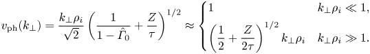 \begin{equation} {{v}_\textrm{ph}(k_{{\perp}})}= \frac{k_\perp \rho_i }{\sqrt{2}} \left(\dfrac{1}{1-\hat{\varGamma}_{0}}+\dfrac{Z}{\tau}\right)^{1/2}\approx \begin{cases} 1 & k_\perp\rho_i\ll1 ,\\ \left({\dfrac{1}{2}+\dfrac{Z}{2\tau}}\right)^{1/2} {k_\perp \rho_i} & k_\perp\rho_i\gg1 . \end{cases} \end{equation}
Finite Larmor radius MHD thus recovers shear-Alfvén waves when  $k_{\perp }\rho _{i}\ll 1$ and (low-
 $\beta$) KAWs when
  $k_{\perp }\rho _{i}\gg 1$. The eigenfunctions of these linear modes, known as the generalised Elsässer potentials, will provide a useful basis for intuitive discussion of the nonlinear problem and turbulence. At wavenumber
  $\boldsymbol {k}$, these are
 \begin{equation} \varTheta_{\boldsymbol{k}}^{{\pm}} ={-}\varOmega_{i}\frac{{v}_\textrm{ph}(k_{{\perp}})}{ k_{{\perp}}^{2}} \frac{\delta n_{e}}{n_{0e}} \mp \frac{A_{\|}}{\sqrt{4{\rm \pi} m_{i} n_{0i} }}.\end{equation}
At large scales  $k_{\perp }\rho _{i}\ll 1$, they have the property
  $\hat {\boldsymbol {z}}\times \boldsymbol {\nabla }_{\perp }\varTheta ^{\pm }=\boldsymbol {Z}^{\pm }=\boldsymbol {u}_{\perp }\pm \boldsymbol {B}_{\perp }/\sqrt {4{\rm \pi} m_{i}n_{0i}}$, where
  $\boldsymbol {Z}^{\pm }$ are the Elsässer variables (Elsasser Reference Elsasser1950).
The utility of  $\varTheta ^{\pm }$ arises from the fact that at large scales (i.e. in the RMHD limit), nonlinear interaction – and thus the turbulent cascade – requires the interaction between
  $\boldsymbol {Z}^{+}$ and
  $\boldsymbol {Z}^{-}$ (equivalently,
  $\varTheta ^{+}$ and
  $\varTheta ^{-}$). Thus, the difference in amplitude of
  $\boldsymbol {Z}^{+}$ and
  $\boldsymbol {Z}^{-}$, which is known as the energy imbalance and is determined by the outer-scale forcing of the plasma, has a strong influence on the properties of the turbulent cascade. We will quantify it in the standard way with
 \begin{equation} \sigma_{c}= \frac{\displaystyle\int\, \textrm{d}^{3}\boldsymbol{x}(|\boldsymbol{Z}^{+}|^{2}-|\boldsymbol{Z}^{-}|^{2})}{\displaystyle\int\, \textrm{d}^{3}\boldsymbol{x}(|\boldsymbol{Z}^{+}|^{2}+|\boldsymbol{Z}^{-}|^{2})}, \end{equation}
so  $\sigma _{c}=\pm 1$ if
  $\boldsymbol {Z}^{-}=0$ or
  $\boldsymbol {Z}^{+}=0$. Although imbalanced RMHD turbulence remains poorly understood (Lithwick, Goldreich & Sridhar Reference Lithwick, Goldreich and Sridhar2007; Chandran Reference Chandran2008; Beresnyak & Lazarian Reference Beresnyak and Lazarian2009; Perez & Boldyrev Reference Perez and Boldyrev2009; Chandran & Perez Reference Chandran and Perez2019; Schekochihin Reference Schekochihin2020), observations show that solar-wind turbulence is usually imbalanced, particularly in near-Sun regions where
  $|\sigma _{c}|\gtrsim 0.9$ (McManus et al. Reference McManus, Bowen, Mallet, Chen, Chandran, Bale, Larson, de Wit, Kasper and Stevens2020). This occurs because Alfvénic perturbations are launched outwards from the corona and only generate an inwards propagating component due to their interaction with background density and field gradients (Velli Reference Velli1993; Chandran & Perez Reference Chandran and Perez2019). Our understanding of plasma turbulence thus remains incomplete without addressing the effect of the imbalance on the flow of energy.
At subion scales ( $k_{\perp }\rho _{i}\gg 1$), the dispersive nature of KAWs makes possible nonlinear interactions between copropagating perturbations (e.g.
  $\varTheta ^{+}$ with
  $\varTheta ^{+}$). This implies that the two components can exchange energy and that a turbulent cascade is, in principle, possible with just one component
  $\varTheta ^{\pm }$ (Cho Reference Cho2011; Kim & Cho Reference Kim and Cho2015; Voitenko & De Keyser Reference Voitenko and De Keyser2016).
2.3. The ‘Helicity Barrier’
Here we argue that the conservation properties of FLR-MHD imply that a turbulent flux of energy cannot proceed in the usual way to small scales (where it needs to get to be dissipated), violating the zeroth law. We term the barrier in the cascade at scales  $l_{\perp }\sim \rho _{i}$, the ‘helicity barrier’.
As discussed above, a necessary (though not sufficient) condition for a turbulent system to satisfy the zeroth law is that it has the ability to transfer energy from the largest scales, where energy is assumed to be injected by external processes, to the smallest, where it can be dissipated. The concept can be formalised by the idea of a turbulent ‘flux’ through scale space; if a system is to remain in statistical steady state, each of its nonlinearly conserved invariants with a source at large scales must have an associated flux.Footnote 3 This flux must be constant across all scales until the invariant can be dissipated. Importantly, this must hold for all nonlinear invariants together: if the flux of one invariant is non-constant and/or insufficient to allow its dissipation, the invariant will change in time, implying that the system is not in steady state. This concept is familiar in the study of two-dimensional (2-D) hydrodynamics, where the dual conservation of energy and enstrophy stops the flux of energy to small scales, causing both energy and enstrophy to build up in time (in the absence of a large-scale dissipation mechanism). The zeroth law can thus be studied in terms of either the dissipation properties, considering how the dissipation rate varies with microphysical dissipation at fixed large-scale conditions (e.g. Pearson et al. Reference Pearson, Yousef, Haugen, Brandenburg and Krogstad2004), or in terms of the large-scale properties, considering how the statistics of the largest scales depend on the microphysical dissipation when the rate of energy injection is fixed. In the following, we examine the conservation laws of FLR-MHD and prove that they do not admit a solution with a constant flux of energy to small perpendicular scales when the energy injection is imbalanced at large scales. This implies that large-scale flows and fields cannot reach steady state through perpendicular dissipation, violating the zeroth law.Footnote 4
2.3.1. Conservation laws of FLR-MHD
The FLR-MHD system has two nonlinearly conserved quadratic invariants, (free) energy and (generalised) helicity. These are most easily and clearly written in terms of the generalised Elsässer variables. The free energy is
 \begin{equation} E=\dfrac{1}{4}\sum_{\boldsymbol{k}}\left( |k_{{\perp}}\varTheta_{\boldsymbol{k}}^{+}|^{2} + | k_{{\perp}}\varTheta_{\boldsymbol{k}}^{-}|^{2} \right),\end{equation}
which reduces to
 \begin{equation} E\approx \frac{1}{4}\int\, \frac{\textrm{d}^{3}\boldsymbol{x}}{V}(|\boldsymbol{Z}^{+}|^{2}+|\boldsymbol{Z}^{-}|^{2})=\frac{1}{2}\int\, \frac{\textrm{d}^{3}\boldsymbol{x}}{V}\left(|\boldsymbol{u}_{{\perp}}|^{2}+\frac{|\boldsymbol{B_{{\perp}}}|^{2}}{4{\rm \pi} n_{0i}m_{i}}\right) \end{equation}
at large scales. The generalised helicity is
 \begin{equation} \mathcal{H}=\frac{1}{4}\sum_{\boldsymbol{k}} \frac{|k_{{\perp}}\varTheta_{\boldsymbol{k}}^{+}|^{2} - |k_{{\perp}}\varTheta_{\boldsymbol{k}}^{-}|^{2}}{{v}_\textrm{ph}(k_{{\perp}})},\end{equation}
which reduces to the MHD cross-helicity at  $k_{\perp }\rho _{i}\ll 1$,
 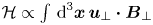 $\mathcal {H}\propto \int \,\textrm {d}^{3}\boldsymbol {x}\,\boldsymbol {u}_{\perp }\boldsymbol {\cdot }\boldsymbol {B}_{\perp }$, and becomes magnetic helicity at
  $k_{\perp }\rho _{i}\gg 1$,
 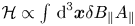 $\mathcal {H}\propto \int \, \textrm {d}^{3}\boldsymbol {x} \delta B_{\|} A_{\|}$.Footnote 5 If the
  $k_{\perp }\rho _{i}\ll 1$ motions dominate over the smaller scales, the energy imbalance is
  $\sigma _{c}\approx \mathcal {H}/E$. We also define the
  $\varTheta ^{\pm }$ ‘energies’,
  $E^{\pm }=\sum _{\boldsymbol {k}}|k_{\perp }\varTheta _{\boldsymbol {k}}^{\pm }|^{2} /4$, along with perpendicular spectra for
  $E$,
$E$,  $\mathcal {H}$, and
  $E^{\pm }$, denoted
  $E(k_{\perp })$,
  $E_{\mathcal {H}}(k_{\perp })$ and
  $E^{\pm }(k_{\perp })$, respectively.
2.3.2. The inevitability of the helicity barrier
Consider the case where energy and helicity are injected at large scales at the rates  $\varepsilon$ and
  $\varepsilon _{\mathcal {H}}$, respectively, with injection imbalance
  $\sigma _{\varepsilon }\equiv |\varepsilon _{\mathcal {H}}|/\varepsilon$. The conservation laws above tell us that in a statistical steady state, there must be a non-zero energy flux
  $\varPi (k_{\perp })$ and helicity flux
  $\varPi _{\mathcal {H}}(k_{\perp })$ to small scales where they can be dissipated. If we further assume that (i) energy transfer due to nonlinearity is significant only for modes with similar scales (locality), and (ii) parallel dissipation is small because eddies are highly elongated along the magnetic field, then
  $\varPi (k_{\perp })$ and
  $\varPi _{\mathcal {H}}(k_{\perp })$ must be constant between the forcing and dissipation scales. In the following argument, based on Alexakis & Biferale (Reference Alexakis and Biferale2018), we assume such a constant-flux solution and find a contradiction, suggesting that this type of solution is not possible in FLR-MHD when
  $\sigma _{\varepsilon }\neq 0$. Fundamentally, the contradiction arises because at large scales
  $\mathcal {H}$ is the RMHD cross-helicity, which undergoes a forward cascade, while at small scales
  $\mathcal {H}$ is magnetic helicity, which undergoes an inverse cascade (Schekochihin et al. Reference Schekochihin, Cowley, Dorland, Hammett, Howes, Quataert and Tatsuno2009; Cho Reference Cho2011; Kim & Cho Reference Kim and Cho2015; Miloshevich et al. Reference Miloshevich, Laveder, Passot and Sulem2021; Pouquet, Stawarz & Rosenberg Reference Pouquet, Stawarz and Rosenberg2020).
Mathematically, the constant-flux solution is
 \begin{gather} \varPi(k_{{\perp}})\simeq \varepsilon\simeq \varepsilon^\textrm{diss}_{{\perp}} = \nu_{n}\sum_{k_{{\perp}}}k_{{\perp}}^{2n} E(k_{{\perp}}), \end{gather}
 \begin{gather}\varPi_{\mathcal{H}}(k_{{\perp}})\simeq\varepsilon_{\mathcal{H}}\simeq \varepsilon^\textrm{diss}_{\mathcal{H},\perp} = \nu_{n}\sum_{k_{{\perp}}}k_{{\perp}}^{2n} E_{\mathcal{H}}(k_{{\perp}}), \end{gather}
where  $\varepsilon ^\textrm {diss}_{\perp }$ and
  $\varepsilon ^\textrm {diss}_{\mathcal {H},\perp }$ are the energy and helicity dissipation rates (we assume hyperviscous dissipation of
  $\delta n_{e}$ and
  $A_{\|}$ of the form
  $\nu _{n}k_{\perp }^{2n}$). This solution satisfies the following inequalities:
 \begin{align} |\varPi_{\mathcal{H}}(k_{{\perp}})|&\simeq \nu_{n}\left| {\sum_{p_{{\perp}}=k_{{\perp}}}^{\infty}p_{{\perp}}^{2n} E_{\mathcal{H}}(p_{{\perp}})}\right| \leqslant \nu_{n} {v}_\textrm{ph}^{{-}1}(k_{{\perp}})\left|{ \sum_{p_{{\perp}}=k_{{\perp}}}^{\infty} p_{{\perp}}^{2n} {v}_\textrm{ph} (p_{{\perp}})E_{\mathcal{H}}(p_{{\perp}})}\right| \nonumber\\ & \leqslant {v}_\textrm{ph}^{{-}1}(k_{{\perp}})\nu_{n} { \sum_{p_{{\perp}}=k_{{\perp}}}^{\infty} p_{{\perp}}^{2n} E(p_{{\perp}})}\simeq {v}_\textrm{ph}^{{-}1}(k_{{\perp}}) \varPi(k_{{\perp}}), \end{align}
where we have used the fact that  ${v}_\textrm {ph}(k_{\perp })$ is a monotonically increasing function of
  $k_{\perp }$, as well as the inequality
 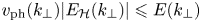 ${v}_\textrm {ph}(k_{\perp }) |E_{\mathcal {H}}(k_{\perp }) |\leqslant E(k_{\perp })$ from (2.7)–(2.9). The ratio of fluxes
 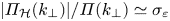 $|\varPi _{\mathcal {H}}(k_{\perp })|/\varPi (k_{\perp })\simeq \sigma _{\varepsilon }$ must thus satisfy
  $\sigma _{\varepsilon }\leqslant 1/{v}_\textrm {ph}(k_{\perp })$ for all
  $k_{\perp }$ above the dissipation scales. But
  $1/{v}_\textrm {ph}(k_{\perp })$ decreases with
  $k_{\perp }$ to arbitrarily small values (
 ${v}_\textrm {ph}\propto k_{\perp }$ at
  $k_{\perp }\rho _{i}\gg 1$). This suggests that, no matter what the injection imbalance, a cascade that tries to proceed to small scales will at some
  $k_{\perp }$ violate the inequality (2.11).Footnote 6 In such a case, the constant-flux solution fails, indicating that the system is unable to thermalise energy and helicity input through small-scale dissipation. We further see that the failure occurs only below the scale where
  $1/{v}_\textrm {ph}(k_{\perp })\simeq \sigma _{\varepsilon }$; this is around
  $k_{\perp }\rho _{i}\simeq 1$ for
  $\sigma _{\varepsilon }\approx 0.7$ but moves to larger scales with increasing
  $\sigma _{\varepsilon }$. This highlights an interesting difference compared with the well known inverse energy cascade of 2-D hydrodynamics (Fjørtoft Reference Fjørtoft1953; Alexakis & Biferale Reference Alexakis and Biferale2018): while standard inverse cascades inhibit forward transfer already at the injection scale, helicity must first travel to microphysical (
 $\rho _{i}$) scales before it hits the barrier. As a consequence, despite FLR effects not influencing directly the nonlinear interactions at MHD scales, they could strongly influence turbulence statistics at those scales by insulating them from the dissipation scales.
3. Numerical experiments
The argument above suggests that it is not possible to have a constant flux of both energy and helicity through the ion-kinetic transition scale. It does not, however, elucidate how the system behaves in the presence of continuous imbalanced injection of energy at large scales. For this, we turn to numerical simulations.
3.1. Numerical set-up
We solve (2.1)–(2.3) using a modified version of the pseudospectral code TURBO (Teaca et al. Reference Teaca, Verma, Knaepen and Carati2009) in a cubic box  $L_{\perp }=L_{z}=L$ with
  $N_{\perp }^{2}\times N_{z}$ Fourier modes. A third-order modified Williamson (Reference Williamson1980) algorithm is used for time stepping. The values of hyperdissipation coefficients
  $\nu _{6\perp }$ and
  $\nu _{6z}$ are chosen based on the numerical resolution, ensuring that the energy spectrum falls off sufficiently rapidly before the resolution cutoff. Fluctuations are stirred at large scales by added forcing terms (
 $f^{n_{e}}$ and
  $f^{A_{\|}}$) in (2.1)–(2.2). This forcing is confined to
  $0< k_{\perp }\leqslant 4{\rm \pi} /L$ and
  $\vert k_{z} \vert = 2{\rm \pi} /L$ and takes the form of negative damping (
 $f^{n_{e}}$ and
  $f^{A_{\|}}$ proportional to the large-scale modes of
  $n_{e}$ and
  $A_{\|}$); this method allows the level of energy and helicity injection (
 $\varepsilon$ and
  $\varepsilon _{\mathcal {H}}$) to be controlled exactly, while producing sufficiently chaotic motions to generate turbulence. While
  $\sigma _{\varepsilon }=\varepsilon _{\mathcal {H}}/\varepsilon$ is thus fixed, the imbalance
  $\sigma _{c}\approx \mathcal {H}/E$ is determined by the turbulence and evolves in time. Initial conditions are random and large-scale with energy
  $E=10\varepsilon \tau _{A}$, where
  $\tau _A=L_z/v_A$ is the Alfvén crossing time. The perpendicular and parallel energy dissipation rates are
  $\varepsilon ^\textrm {diss}_{\perp }=\nu _{6\perp }\sum _{k_{\perp },k_{z}}k_\perp ^6 E(k_\perp ,k_z)$ and
  $\varepsilon ^\textrm {diss}_{z}=\nu _{6z}\sum _{k_{\perp },k_{z}}k_z^6 E(k_\perp ,k_z)$, where
  $E(k_\perp ,k_z)$ is the 2-D energy spectrum (in steady state, if it exists, we would have
  $\varepsilon =\varepsilon ^\textrm {diss}=\varepsilon ^\textrm {diss}_{\perp }+\varepsilon ^\textrm {diss}_{z}$). Simulations are run across a range of resolutions up to
  $N_{\perp }=N_{z}=2048$. For the highest-resolution cases, we use a recursive refinement procedure, restarting a lower-resolution case at twice the resolution and running until
  $\varepsilon ^\textrm {diss}_{\perp }$ converges in time; this dramatically reduces the computational cost to enable otherwise unaffordable simulations. All simulations use
  $Z=1$ and
  $\tau =0.5$ (so that the ion-sound radius is equal to
  $\rho _{i}$).
3.2. Results
Figure 3 demonstrates how imbalanced FLR-MHD turbulence violates the zeroth law of turbulence. Figure 3(a) shows the normalised perpendicular dissipation rate  $\varepsilon ^\textrm {diss}_{\perp }/\varepsilon$ in the saturated state of 16 FLR-MHD simulations with
  $\sigma _{\varepsilon }=0.88$,
  $\rho _{i}=0.02L_{\perp }$ and varying perpendicular hyperdissipation
  $\nu _{6\perp }$. The simulations have fixed
  $\nu _{6z}$, resolution
  $N_{\perp }=N_{z}=256$ (or
  $N_{\perp }=512$ for the four lowest-
 $\nu _{6\perp }$ cases), and were run by restarting from the saturated state of the
  $1/\nu _{6\perp }\simeq 3\times 10^{10}$ simulation (denoted by the purple star), which will be discussed in detail below. We see a precipitous drop in
  $\varepsilon ^\textrm {diss}_{\perp }$ for
  $1/\nu _{6\perp }\gtrsim 10^{8}$, which signifies that the turbulent energy flux cannot proceed to small perpendicular scales for small
  $\nu _{6\perp }$. This is the signature of the helicity barrier predicted above in § 2.3.2: if the scale at which the energy dissipates due to
  $\nu _{6\perp }$ is such that the inequality (2.11) is violated, the constant perpendicular flux solution cannot hold.
The vertical dashed line in figure 3(a) shows the critical value  $\nu _{6\perp }^\textrm {crit}$ needed to set the perpendicular dissipation scale of RMHD turbulence equal to the scale
  $k_{\perp }^\textrm {crit}\simeq 22.4(2{\rm \pi} /L_{\perp })$ where
  $1/{v}_\textrm {ph}(k_{\perp }^\textrm {crit})=\sigma _{\varepsilon }=0.88$. We estimate
  $\nu _{6\perp }^\textrm {crit}$ from
  $\nu _{6\perp }k_\perp ^6\sim k_\perp Z^-_{k_\perp }$, where
  $Z^-_{k_\perp }\sim Z^-_{0}(k_\perp L_\perp )^{-1/4}$ is the typical variation in
  $Z^-$ across scale
  $k_\perp ^{-1}$, and the outer-scale amplitude
  $Z^-_{0}$ is taken from saturated state of the similar RMHD simulation shown in figure 5. If
  $\nu _{6\perp }>\nu _{6\perp }^\textrm {crit}$, the cascade can dissipate in the standard way on hyperdissipation, setting up an imbalanced RMHD cascade; if
  $\nu _{6\perp }<\nu _{6\perp }^\textrm {crit}$, the inequality (2.11) applies, stopping the cascade before it reaches small perpendicular scales and causing
  $\varepsilon ^\textrm {diss}_{\perp }\ll \varepsilon$.
This inability of the perpendicular cascade to process injected energy into perpendicular dissipation suggests that the parallel dissipation must play a role. This is surprising given that parallel dissipation is usually neglected in magnetised-turbulence theories because the increasing elongation of eddies at smaller scales generally implies  $\varepsilon ^\textrm {diss}_{\perp }\gg \varepsilon ^\textrm {diss}_{z}$. In figure 3(b), we show the turbulent-energy saturation amplitude
  $E_\textrm {sat}$ as a function of the parallel hyperdissipation
  $\nu _{6z}$. These simulations are again forced with injection imbalance
  $\sigma _{\varepsilon }=0.88$ and use a lower resolution
  $N_{\perp }=64$ and
  $64\leqslant N_{z}\leqslant 256$ (with
  $N_{z}$ chosen as appropriate for each
  $\nu _{6z}$) because of the long saturation times. The perpendicular dissipation is fixed and sufficiently small for there to be a helicity barrier. We compare FLR-MHD turbulence with
  $\rho _{i}=0.1L_{\perp }$ (coloured points) with RMHD turbulence (
 $\rho _{i}=0$, black points) to demonstrate the significant role played by FLR effects. The difference is obvious: FLR-MHD turbulence saturates at much larger amplitudes, which increase with decreasing dissipation; larger amplitudes are associated with longer saturation times (see inset, cf. Miloshevich et al. (Reference Miloshevich, Laveder, Passot and Sulem2021)). This dependence of saturation time and large-scale properties on
  $\nu _{6z}$ shows that imbalanced FLR-MHD turbulence violates the zeroth law of turbulence with respect to the parallel, as well as the perpendicular, dissipation.
The implications of these findings are twofold. First, in order to saturate, imbalanced FLR-MHD turbulence must access small-scale parallel physics, escaping the ordering assumptions ( $l_{\|}\gg l_{\perp }$) used to derive the FLR-MHD model in the first place. This suggests that detailed properties of the saturated state achieved by this model are not relevant to real physical systems. Secondly, when the helicity barrier halts the perpendicular cascade, the system does not develop a true parallel cascade that can process the energy and helicity input into parallel dissipation. Rather, its saturated amplitude depends directly on the microphysical parallel dissipation (the specific
  ${\sim }\nu _{6z}^{-1/4}$ dependence is explained below), suggesting that in the limit of vanishing parallel dissipation, the turbulence would fail to saturate completely.
These highly unusual characteristics motivate a more thorough exploration of imbalanced FLR-MHD turbulence. Below and in figures 1–2, we present detailed simulation results to help explain the effect of the helicity barrier and its potential relevance to space plasmas. We compare imbalanced FLR-MHD with an equally imbalanced RMHD simulation and balanced FLR-MHD, all at the same  $\varepsilon$. To aid discussion, we break the time evolution into three phases: first, a transient phase during which small-scale motions are produced from the initial conditions; next, a pseudo-stationary phase, which is the long phase of slow energy growth (seen in the inset of figure 3b) that occurs due to the helicity barrier; and finally, saturation, when
  $\varepsilon \approx \varepsilon ^\textrm {diss}_{\perp }+\varepsilon ^\textrm {diss}_{z}$ and
  $\partial _{t}E\approx 0$. During the pseudo-stationary phase and saturation, the helicity barrier creates a sharp break in the perpendicular spectrum at a wavenumber that we will denote
  $k_{\perp }^{*}$.
3.2.1. The effect of the helicity barrier
Figures 4–6 show the time evolution of the energy, dissipation  $\varepsilon ^\textrm {diss}_{\perp ,\|}$, energy spectra
  $E^{\pm }(k_{\perp })$ and total energy flux
  $\varPi (k_{\perp })$, comparing imbalanced FLR-MHD at
  $\sigma _{\varepsilon }=0.88$ and
  $\rho _{i} = 0.02 L_{\perp }$Footnote 7 with balanced FLR-MHD (
 $\sigma _{\varepsilon }=0$,
  $\rho _{i} = 0.02 L_{\perp }$) and imbalanced RMHD (
 $\sigma _{\varepsilon }=0.88$,
  $\rho _{i} = 0$). These simulations, which have a resolution of
  $N_{\perp }=N_{z}=256$, are used as low-resolution seeds (starting at
  $t\approx 18\tau _{A0}$) for the recursive resolution refinement that allows us to reach
  $N_{\perp }=N_{z}=2048$ in figure 2 (the full time evolution is only computationally accessible at modest resolution). Let us first describe the balanced FLR-MHD and imbalanced RMHD cases in order to highlight the effect of the helicity barrier.

Figure 4. Energy and dissipation properties from a set of simulations at resolution  $N_\perp =N_z=256$. Panel (a) compares the time evolution of energy in imbalanced FLR-MHD (
 $\sigma _{\varepsilon }=0.88$,
  $\rho _i=0.02L$) with balanced FLR-MHD (
 $\sigma _{\varepsilon }=0$,
  $\rho _i=0.02L$) and imbalanced RMHD (
 $\sigma _{\varepsilon }=0.88$,
  $\rho _i=0$). The stars indicate the time from which the higher-resolution simulations of figures 1–2 were initialised. Panel (b) shows
  $\varepsilon ^\textrm {diss}_{\perp }$ (solid lines) and
  $\varepsilon ^\textrm {diss}_{z}$ (dotted lines) for each case, to show that saturation is reached through parallel dissipation (unlike in balanced turbulence and in imbalanced RMHD). Panel (c) shows the (
 $k_{\perp },k_{z}$) dissipation spectrum in the saturated state of imbalanced FLR-MHD, illustrating that dissipation occurs primarily at the perpendicular break scale (
 $k_{\perp }^{*}\rho _{i}\simeq 0.15$) at high
  $k_{z}$.

Figure 5. Time evolution of the spectra,  $E^\pm (k_\perp )$, for the simulations shown in figure 4, comparing imbalanced FLR-MHD (a), balanced FLR-MHD (b) and imbalanced RMHD (c). Individual spectra are shown at times spaced by
  $t=0.1\tau _A$, as indicated by the colour. While the spectrum converges rapidly in balanced FLR-MHD and imbalanced RMHD turbulence, the spectra of imbalanced FLR-MHD turbulence continue to evolve until
  $t\simeq 200\tau _{A}$, with the break continuously moving to larger scales.

Figure 6. Time evolution of the normalised energy flux  $\varPi (k_{\perp })/\varepsilon$ for the simulations of figures 4–5, comparing imbalanced FLR-MHD (top panel) and balanced FLR-MHD (bottom panel). The colouring is the same as in figure 5. While balanced FLR-MHD turbulence shows the expected near-constant flux to small scales (where it is dissipated), imbalanced FLR-MHD turbulence is characterised by wild fluctuations in
  $\varPi$ (note different ordinate scale and the position of the grey line at
  $\varPi =\varepsilon$), which, with time, are increasingly confined to large scales. The time-dependent wavenumber of the break (
 $k_{\perp }^{*}$) is shown with the coloured vertical lines. We also show, with
  $k_{\nu _\perp }$, the scale at which
  $\varPi$ is equal to the perpendicular dissipation flux (brown lines) in each simulation. The small flux
  $\varPi \ll \varepsilon$ at smaller scales provides direct evidence for the existence of the helicity barrier.
The balanced FLR-MHD simulation reaches saturation after a transient phase lasting several  $\tau _{A}$, exhibiting a
  $\sim \!k_{\perp }^{-3/2}$ spectrum at large scales (figure 5) and constant flux of energy to small scales (figure 6) where it is dissipated with
  $\varepsilon ^\textrm {diss}_{\perp }\gg \varepsilon ^\textrm {diss}_{z}$ (figure 4b). While the transition to KAW turbulence (
 $\sim \!k_{\perp }^{-2.8}$) at
  $k_{\perp }\rho _{i}\simeq 1$ is superseded by the dissipation range at
  $N_{\perp }=256$, it is clearly visible in the
  $N_{\perp }=2048$ spectrum in figure 2. The imbalanced RMHD simulation is similar, although it is slower to saturate, reaching steady state by
  $\tau _{A}\simeq 40$, with a
  $\sim \!k_{\perp }^{-3/2}$ spectrum in
  $E^{+}$ and
  $E^{-}$ (figure 5) and energy fluxes to small perpendicular scales (not shown). The larger saturated energy arises because the cascade time
  $\tau _\textrm {cas}$ is larger in imbalanced turbulence due to its slower nonlinear interactions (Lithwick et al. Reference Lithwick, Goldreich and Sridhar2007; Chandran Reference Chandran2008), implying
  $E_\textrm {sat}\sim \varepsilon \tau _\textrm {cas}$ is larger with fixed
  $\varepsilon$. As
  $E$ grows, the parallel outer scale
  $l_{\|0}$ decreases due to critical balance (
 $l_{\|0}\sim L_{\perp }v_{A}/E^{1/2}$), which causes a modest parallel dissipation (
 $\varepsilon ^\textrm {diss}_{z}\simeq 0.3 \varepsilon ^\textrm {diss}$) observed in RMHD for the chosen parameters (figure 4b). This disappears at either lower
  $\varepsilon$ and/or higher resolution.
Imbalanced FLR-MHD turbulence is markedly different from both its balanced counterpart and imbalanced RMHD turbulence. As noted above, the latter is especially remarkable because FLR-MHD is identical to RMHD at  $k_{\perp }\rho _{i}\ll 1$, and
  $\rho _{i}$ (vertical line in figure 5) lies only slightly above the resolution cutoff (where perpendicular dissipation dominates) at these parameters. After an initial transient phase (
 $t\lesssim 5\tau _{A}$) when its evolution is similar to RMHD, the system forms a sharp spectral break at
  $k_{\perp }^{*}$, and the pseudo-stationary phase begins. During this phase, the outer-scale energy in
  $E^{+}(k_{\perp })$ grows in time, while the spectral break, which lies near
  $k_{\perp }^{*}\rho _{i}\simeq 1$ at early times, migrates to larger scales. That this break is due to the ‘helicity barrier’ can be seen directly in the energy flux (figure 6): as time goes on,
  $\varPi (k_{\perp })$ is confined to increasingly large scales (broadly matching
  $k_{\perp }^{*}$, shown with coloured lines), as well as fluctuating wildly compared with balanced turbulence. Clearly,
  $\varPi \ll \varepsilon$ for
  $k_{\perp }>k_{\perp }^{*}$, which explains the continual increase in
  $E$ with time during this phase. The subdominant mode's spectrum
  $E^{-}(k_{\perp })$ behaves quite differently to
  $E^{+}(k_{\perp })$, undergoing a modest decrease at earlier times and saturating well before
  $E^{+}$. This implies that the energy imbalance
  $\sigma _{c}$ increases with time during the pseudo-stationary phase. Interestingly, the
  $E^{-}$ cascade appears agnostic to the break in
  $E^{+}(k_{\perp })$ and proceeds to small perpendicular scales. This is consistent with the observation that the saturated perpendicular energy dissipation seems to approach
  $\varepsilon ^\textrm {diss}_{\perp }\approx 2\varepsilon ^{-}=\varepsilon (1-\sigma _{\varepsilon })$ in the pseudo-stationary phase (a result that has been confirmed at higher resolution and at other
  $\sigma _{\varepsilon }$). This suggests a form of ‘flux pinning’ (
 $\varepsilon ^{-}\approx \varepsilon ^{+}$), whereby the energy flux to small scales is determined by the requirement of a near-balanced KAW cascade (as seen in figure 2), which thus avoids the problems associated with the inverse cascade of helicity. The amplitude of this cascade appears to be limited by the availability of
  $\varTheta ^{-}$ fluctuations arriving from the inertial range.Footnote 8
The saturation mechanism in imbalanced FLR-MHD is fundamentally different from the balanced case or from imbalanced RMHD turbulence, because  $\varPi (k_{\perp })$ at
  $k_{\perp }\gtrsim k_{\perp }^{*}$ remains limited to
  ${\simeq }2\varepsilon ^{-}$, no matter what the turbulence amplitude. Saturation finally occurs – at
  $t\approx 200\tau _{A}$ with energy imbalance reaching
  $\sigma _{c}\approx 0.999$ for the FLR-MHD simulation of figures 4–6 – once eddies of perpendicular scale
  $k_{\perp }^{*}$ reach sufficiently large amplitudes and small parallel scales to dissipate through parallel hyperdissipation (figure 4). Our simulations indicate that this generation of small parallel scales occurs due to critical balance rather than through an independent parallel cascade to small
  $l_{\|}$ at fixed
  $k_{\perp }$ (which would imply a
  $\nu _{6z}$-independent
  $E_\textrm {sat}$). We can thus estimate the saturation amplitude using
  $l_{\|}(k_{\perp })\sim l_{\|0} (L_{\perp }k_{\perp })^{-1/2}$ and
  $Z^{+}_{k_{\perp }}\sim E^{1/2}(L_{\perp }k_{\perp })^{-1/4}$, where
  $Z^{+}_{k_{\perp }}$ is the typical variation in
  $\boldsymbol {Z}^{+}$ across scale
  $k_{\perp }^{-1}$ and
  $l_{\|}(k_{\perp })$ is the corresponding parallel correlation length (Mallet & Schekochihin Reference Mallet and Schekochihin2017). Noting that saturation occurs at
  $\nu _{6z}l_{\|}(k_{\perp }^{*})^{-6}(Z^{+}_{k_{\perp }^{*}})^{2}\sim \varepsilon$ and
  $l_{\|0}\sim L_{\perp }v_{A}/E_\textrm {sat}^{1/2}$, we find
 \begin{equation} E_\textrm{sat}\sim (\varepsilon/\nu_{6z})^{{-}1/4} (k_{{\perp}}^{*} L_{{\perp}})^{{-}5/8}(v_{A}L_{{\perp}})^{3/2}. \end{equation}
The  $\nu _{6z}^{-1/4}$ scaling is approximately satisfied by the simulations in figure 3 (which all saturate with similar
  $k_{\perp }^{*}$ near the forcing scales), while the 2-D dissipation spectrum in figure 4(c) confirms directly that most dissipation occurs at small
  $l_{\|}$ on
  $k_{\perp }^{*}$-scale eddies. Figure 4(c) also shows the critical-balance scaling
  $l_{\|}\sim k_{\perp }^{-1/2}$ (although note that
  $k_{z}$ rather than
  $k_{\|}\sim l_{\|}^{-1}$ is plotted) and the finite
  $\varepsilon ^\textrm {diss}_{\perp }$ at larger
  $k_{\perp }$ from flux leakage through the barrier. As mentioned above, this saturation mechanism is unphysical: by growing to
  $\varepsilon ^\textrm {diss}_{z}>\varepsilon ^\textrm {diss}_{\perp }$, the system is trying to break the
  $l_{\|}\ll l_{\perp }$ ordering used to derive FLR-MHD. Nonetheless, only with this basic understanding of why the system saturates can we evaluate how the helicity barrier might evolve in more realistic scenarios.
Finally, it is worth noting an interesting feature of the MHD-scale ( $k_{\perp }< k_{\perp }^{*}$) turbulence in the pseudo-stationary phase: even though most of the energy input is unable to be thermalised during this phase, causing
  $E^{+}$ to grow in time, the spectrum remains approximately
  $E^{+}(k_{\perp })\sim k_{\perp }^{-3/2}$ for
  $k_{\perp }< k_{\perp }^{*}$ (see figure 2 and the inset of figure 7). This is in contrast to standard (e.g. hydrodynamic) turbulence with insufficient small-scale dissipation, which usually forms a thermal spectrum that is an increasing function of
  $k_{\perp }$ (see e.g. Cichowlas et al. (Reference Cichowlas, Bonaïti, Debbasch and Brachet2005) and Frisch et al. (Reference Frisch, Kurien, Pandit, Pauls, Ray, Wirth and Zhu2008), for a study of the truncated Euler equations). We speculate that this occurs because, even in the presence of a helicity barrier,
  $\varTheta ^{-}$ still nonlinearly cascades to dissipate at small scales (see discussion above), thus behaving in a way similar to RMHD. But, for
  $k_{\perp }\rho _{i}<1$ where
  $\boldsymbol {Z}^{-}\approx \hat {\boldsymbol {z}}\times \boldsymbol {\nabla }_{\perp }\varTheta ^{-}$, the nonlinear cascade of
  $\varTheta ^{+}$ is governed by
  $\varTheta ^{-}$ because only counter-propagating waves interact in RMHD. This suggests that
  $E^{+}$ does not form a thermal spectrum because of the
  $\varTheta ^{-}$ cascade, although the phenomenology of the cascade in the presence of a barrier remains highly uncertain. Nonetheless, our simulations robustly show that both
  $E^{+}(k_{\perp })$ and
  $E^{-}(k_{\perp })$ scale as
  ${\sim }k_{\perp }^{-3/2}$, as observed in the solar wind (Chen Reference Chen2016; Chen et al. Reference Chen, Bale and Bonnell2020).

Figure 7. Position of the break  $k_{\perp }^{*}\rho _{i}$ versus the energy imbalance (
 $1-\sigma _{c}$) for a number of
  $N_{\perp }=N_{z}=256$ simulations with different injection imbalances
  $\sigma _{\varepsilon }$. As
  $\sigma _{c}(t)$ grows in time due to the helicity barrier, there is concurrent decrease in
  $k_{\perp }^{*}$, with no obvious dependence on the helicity injection
  $\sigma _{\varepsilon }=\varepsilon _{\mathcal {H}}/\varepsilon$ or other time dependence. The black line shows the empirical fit (3.2), the star shows the fit for figure 2, and the greyed out region indicates where
  $k_{\perp }^{*}$ gets within a factor of 2 of the forcing scale (
 $k_{\perp }^{*}< 4\times 2{\rm \pi} /L$). The inset shows a histogram of the fitted spectral slope
  ${\sim }k_{\perp }^{-\alpha }$ above and below the break for the
  $\sigma _{\varepsilon }=0.88$ simulation of figure 5 (the averages are
  $\langle \alpha \rangle \approx 1.67$ above the break and
  $\langle \alpha \rangle \approx 3.8$ below the break).
3.2.2. The ion spectral break
For testing of the helicity-barrier hypothesis against observations, it is of interest to understand the position and spectral slope of the ion-kinetic transition region around  $\rho _{i}$ scales. Given the unphysical saturation mechanism in our simulations, we hypothesise that the pseudo-stationary phase is of more relevance to realistic space plasmas and that the ‘instantaneous’ state of turbulence during that stage can be characterised by the energy imbalance
  $\sigma _{c}(t)$ and the injection imbalance
  $\sigma _{\varepsilon }$, i.e. that the time history of the growth is unimportant. Figure 7 shows
  $k_{\perp }^{*} \rho _{i}$ versus imbalance (
 $1-\sigma _{c}$) for simulations with four different
  $\sigma _{\varepsilon }$ at
  $N_{\perp }=N_{z}=256$, as well as the spectral slopes (
 ${\sim }k_{\perp }^{-\alpha }$) above and below
  $k_{\perp }^{*}$ for
  $\sigma _{\varepsilon }=0.88$ (inset; the values of
  $\alpha$ are obtained via a broken-power-law fit (Astropy Collaboration 2013)). We see good correlation of
  $k_{\perp }^{*}$ to
  $\sigma _{c}(t)$, approximately
 \begin{equation} k_{{\perp}}^{*} \rho_{i} \simeq (1-\sigma_{c})^{1/4},\end{equation}
with little dependence on the injected flux. We have also confirmed that the  $1/4$-power scaling (although not the numerical coefficient) is robust to the order of the parallel hyperdissipation (it also holds if
  $\nu _{6z}=0$; not shown). Spectral slopes in the ion-kinetic transition range (
 $k_{\perp }> k_{\perp }^{*}$) are seen to vary more than in the MHD range (
 $k_{\perp }< k_{\perp }^{*}$) and are very steep,
  $\alpha \simeq 4$, in good agreement with PSP observations (Bowen et al. Reference Bowen, Mallet, Bale, Bonnell, Case, Chandran, Chasapis, Chen, Duan and de Wit2020a).
4. Discussion
Our simulations show a dramatic difference in imbalanced Alfvénic turbulence depending on whether or not energy can be dissipated at spatial scales above the ion-gyroradius scale. If it can, turbulence proceeds in a relatively conventional way, with energy reaching small perpendicular scales where it is thermalised by (hyper)-dissipation. If it cannot, the helicity barrier blocks the cascade at  $k_{\perp }^{*}\rho _{i}\lesssim 1$, only a small proportion (
 ${\simeq }2\varepsilon ^{-}$) of the energy can reach the smallest perpendicular scales where it would heat electrons, while
  $E^{+}$ grows with time until it becomes so large that modes at
  $k_{\perp }^{*}$ (which itself moves to large scales) dissipate on the parallel viscosity. The latter effect is unphysical – FLR-MHD is derived by assuming
  $l_{\|}\gg l_{\perp }$ – so the obvious question that arises is what would happen in a real plasma such as the solar wind. In order for the barrier to lose its importance for large-scale dynamics, some mechanism must either remove nearly all of the helicity in the system, thus allowing the energy to be channelled into the small-scale KAW cascade, or significantly dissipate both energy and helicity at or above the scale of the barrier (as the parallel dissipation does in FLR-MHD). Presumably, a real plasma will find a way to accomplish one of these feats – the question is which, and what conditions (e.g. fluctuation amplitudes) are required for it to do so. A definitive answer will have to wait either for observations or for high-resolution six-dimensional kinetic simulations, but we can nonetheless speculate on possibilities.
The first possibility is that there exists another perpendicular dissipation mechanism that stops the formation of a helicity barrier in the first place. Within the gyrokinetic ordering  $l_{\perp }\ll l_{\|}$, because the low ion-thermal speed at
  $\beta _{i}\ll 1$ implies that Alfvénic energy is incapable of heating ions significantly at any scale, there are in principle three possible such mechanisms: electron Landau damping; electron-inertial effects; and interactions with the compressive cascade. Electron Landau damping is modest at
  $k_{\perp }\rho _{i}\sim 1$ when
  $1\gg \beta \gg m_{e}/m_{i}$ (e.g. normalised damping of
  ${\simeq }1\,\%$ at
  $\beta \simeq 0.1$, see Howes et al. (Reference Howes, Cowley, Dorland, Hammett, Quataert and Schekochihin2006)), while electron-inertial effects change the equations only once
  $k_{\perp }d_{e}\sim 1$; so, neither of these effects seems capable of damping substantial helicity or energy. A compressive cascade, although it cannot exchange energy with Alfvénic motions (Schekochihin et al. Reference Schekochihin, Kawazura and Barnes2019), does break helicity conservation around
  $k_{\perp }\rho _{i}\sim 1$; however, in order to have a significant effect, the compressive and Alfvénic cascades must have similar energy contents, which is not generally observed in the solar wind (Bruno & Carbone Reference Bruno and Carbone2013; Chen Reference Chen2016; Chen et al. Reference Chen, Bale and Bonnell2020). Beyond gyrokinetics, cyclotron damping, although perhaps important in the KAW range (Arzamasskiy et al. Reference Arzamasskiy, Kunz, Chandran and Quataert2019), requires Larmor-frequency fluctuations, a requirement that is difficult to reach for
  $k_{\perp }\rho _{i}\lesssim 1$ fluctuations with
  $l_{\|}\ll \rho _{i}$. Stochastic-ion heating (Chandran et al. Reference Chandran, Li, Rogers, Quataert and Germaschewski2010) is more promising – it can dissipate significant turbulent energy at
  $k_{\perp }\rho _{i}\sim 1$ so long as the fluctuation amplitude there exceeds a critical threshold
  ${\simeq }0.2\beta ^{1/2}$ – perhaps acting as a dissipation ‘switch’ as the amplitude grows. It is worth noting, however, that if a
  $k_{\perp }^{*}\rho _{i}\lesssim 1$ barrier has formed before significant stochastic heating occurs, this reduces the
  $\rho _{i}$-scale turbulence amplitude substantially, which also reduces the heating efficiency.
If the aforementioned perpendicular dissipation mechanisms fail to dissolve the barrier, it is also possible that – even in a real plasma – large-scale energy cannot dissipate, either growing until significant power reaches small parallel scales (of order  $d_{i}$ or
  $\rho _{i}$) or, in stratified environments such as the solar wind (Chandran & Perez Reference Chandran and Perez2019), propagating and growing without dissipation until wave reflection causes the imbalance to decrease enough to allow the cascade to proceed. In the former case, various other, non-gyrokinetic dissipation avenues are made available to the plasma; for example, other cascade channels (Saito et al. Reference Saito, Gary, Li and Narita2008; Meyrand & Galtier Reference Meyrand and Galtier2012) and ion-cyclotron damping, which could absorb the cascade's energy (much like the parallel hyperdissipation in our simulations). Interestingly, PSP has observed surprisingly high power in
  $l_{\|}\sim \rho _{i}$ ion-cycloton waves (Huang et al. Reference Huang, Zhang and Sahraoui2020; Bowen et al. Reference Bowen, Mallet, Huang, Klein, Malaspina, Stevens, Bale, Bonnell, Case and Chandran2020b), which may be a signature of this mechanism. Further, Duan et al. (Reference Duan, He, Bowen, Woodham, Wang, Chen, Mallet and Bale2021) find a sharp drop in the wavevector anisotropy
  $l_\|(l_\perp )$ around the break scale, indicating that the dynamics are generating small parallel scales faster than small perpendicular scales. Finally, magnetic reconnection may play an important role by enabling non-local energy or helicity transfers (Loureiro & Boldyrev Reference Loureiro and Boldyrev2017; Mallet et al. Reference Mallet, Schekochihin and Chandran2017; Vech et al. Reference Vech, Mallet, Klein and Kasper2018); although reconnection is possible within FLR-MHD, it is necessary to include electron-inertial effects to capture this physics properly.
4.1. A critical imbalance?
Our theoretical arguments for helicity-barrier formation, which relied on conservation of energy and helicity in FLR-MHD, suggest that a barrier should form with any injected imbalance  $\sigma _{\varepsilon }$, but with the constant flux solution failing at smaller scales for smaller
  $\sigma _{\varepsilon }$, viz., for
  $1/ {v}_\textrm {ph}(k_{\perp })<\sigma _{\varepsilon }$.Footnote 9 We have confirmed this prediction numerically down to
  $\sigma _{\varepsilon }\simeq 0.3$ (not shown). It is challenging to observe at yet smaller
  $\sigma _{\varepsilon }$, both because very small scales (compared with
  $\rho _{i}$) must be resolved, and because a large proportion of the energy flux (
 ${\simeq } 2\varepsilon ^{-}$) is not affected by the barrier, making the resulting growth in energy rather slow. It is, however, clear that non-FLR-MHD effects will give rise to a critical
  $\sigma _{\varepsilon }$, below which there is no barrier. Finite Larmor radius MHD breaks down at
  $d_{e}$ scales and helicity is no longer conserved, implying that the helicity barrier will likely not form if
 \begin{equation} \sigma_{\varepsilon}\lesssim \frac{1}{{v}_\textrm{ph}(d_{e}^{{-}1})}\sim \frac{d_{e}}{\rho_{i}}=\frac{Z}{\sqrt{\tau}} \sqrt{\frac{m_{e}}{m_{i}}}\,\beta_{e}^{{-}1/2} \end{equation}
(the latter estimates assume  $\beta _{e}\gg m_{e}/m_{i}$). The discussion of the previous paragraph also suggests that other effects (e.g. stochastic-ion heating) would further increase the minimal
  $\sigma _{\varepsilon }$ for which the barrier forms, by dissipating some helicity or energy. Measurement of this critical imbalance, along with improved theoretical understanding of helicity-barrier formation and dissolution, is left to future studies.
4.2. Implications for the solar wind
The qualitative agreement of our FLR-MHD energy spectra with those observed in the solar wind is highly suggestive. As far as we are aware, no previous numerical simulations have been able to produce similar double-kinked spectra. The position, shape and cause of the ion-kinetic transition has been a decades-long puzzle with numerous proposed explanations (Schekochihin et al. Reference Schekochihin, Cowley, Dorland, Hammett, Howes, Quataert and Tatsuno2009; Sahraoui et al. Reference Sahraoui, Goldstein, Belmont, Canu and Rezeau2010; Meyrand & Galtier Reference Meyrand and Galtier2012; Lion, Alexandrova & Zaslavsky Reference Lion, Alexandrova and Zaslavsky2016; Voitenko & De Keyser Reference Voitenko and De Keyser2016; Mallet et al. Reference Mallet, Schekochihin and Chandran2017; Woodham et al. Reference Woodham, Wicks, Verscharen and Owen2018); observations show widely varying break positions and slopes (Leamon et al. Reference Leamon, Smith, Ness, Matthaeus and Wong1998) often followed by a spectral flattening at yet smaller scales (Sahraoui et al. Reference Sahraoui, Goldstein, Robert and Khotyaintsev2009; Bowen et al. Reference Bowen, Mallet, Bale, Bonnell, Case, Chandran, Chasapis, Chen, Duan and de Wit2020a; Duan et al. Reference Duan, He, Bowen, Woodham, Wang, Chen, Mallet and Bale2021). In addition, larger-scale transitions to steeper spectra correlate with higher-amplitude fluctuations, lower  $\beta$, higher proton-scale magnetic helicity and fast-wind regions (Smith et al. Reference Smith, Hamilton, Vasquez and Leamon2006; Bruno, Trenchi & Telloni Reference Bruno, Trenchi and Telloni2014; Vech et al. Reference Vech, Mallet, Klein and Kasper2018; Zhao et al. Reference Zhao, Lin, Wang, Wu, Feng, Liu, Zhao and Li2020), the latter of which is known to be more imbalanced than the slow wind. Each of these observations is well explained by the helicity-barrier hypothesis, at least qualitatively: we reproduce double-kinked spectra with the first break at a non-universal scale above
  $k_{\perp }\rho _{i}=1$, while steeper spectra and larger-scale breaks result from the energy growing in time (figure 5). It is also worth noting that direct measurement of the turbulent energy flux in the solar wind has found the surprising result that the
  $\boldsymbol {Z}^{+}$ flux seems to reverse at large imbalance (Smith et al. Reference Smith, Stawarz, Vasquez, Forman and MacBride2009); although not fully explained by our simulations (given that our forcing injects energy only at large scales), the result does indicate the presence of a critical imbalance that controls key features of the cascade. Future observations, combined with more realistic simulations, will provide more stringent tests of the theory.
More generally, if the helicity barrier proves to be a robust feature of plasma turbulence, we see a number of interesting implications. Turbulence is believed to contribute importantly to solar-wind heating (Dmitruk et al. Reference Dmitruk, Matthaeus, Milano, Oughton, Zank and Mullan2002), so the requirement that it build up significantly in amplitude before being able to dissipate may have consequences for global heliospheric models (Verdini & Velli Reference Verdini and Velli2007; Chandran & Hollweg Reference Chandran and Hollweg2009). It is also interesting to ask about the plausible relevance to the sudden large-scale field reversals, or ‘switchbacks’, observed ubiquitously by PSP (Bale et al. Reference Bale, Badman, Bonnell, Bowen, Burgess, Case, Cattell, Chandran, Chaston and Chen2019; Kasper et al. Reference Kasper, Bale, Belcher, Berthomier, Case, Chandran, Curtis, Gallagher, Gary and Golub2019): if switchbacks form in situ due to wave growth in the expanding plasma (Squire, Chandran & Meyrand Reference Squire, Chandran and Meyrand2020), their existence relies on the dominance of growth over dissipation through turbulence. Halting energy dissipation via the helicity barrier could thus favour the development of sharp, large-amplitude structures, as observed. Finally, and more generally, the helicity barrier reveals yet another way that weakly collisional plasmas confound standard intuition about their thermodynamics. While Joule found that water or mercury possess a well-defined heat capacity, independent of how the fluid is heated, heating of ions and electrons in a plasma depends not just on bulk properties such as  $T_{e}/T_{i}$ or
  $\beta$ (Howes et al. Reference Howes, Cowley, Dorland, Hammett, Quataert and Schekochihin2008; Kawazura, Barnes & Schekochihin Reference Kawazura, Barnes and Schekochihin2019), but also, quite sensitively, on how it is stirred. While the influence of the driving compressibility on heating is already known (Schekochihin et al. Reference Schekochihin, Kawazura and Barnes2019; Kawazura et al. Reference Kawazura, Schekochihin, Barnes, TenBarge, Tong, Klein and Dorland2020), we see that driving imbalance should also have a strong effect, by halting the flow of Alfvénic energy to electron scales. The helicity barrier is thus expected to narrow yet further the range of plasma conditions under which electrons are heated preferentially to ions.
Acknowledgements
The authors wish to acknowledge the use of New Zealand eScience Infrastructure (NeSI) high performance computing facilities and consulting support as part of this research. This work was partially performed using HPC resources from GENCI-CINES (Grant 2019-A0060510871).
Editor Francesco Califano thanks the referees for their advice in evaluating this article.
Funding
Support for R.M. and J.S. was provided by Rutherford Discovery Fellowship RDF-U001804 and Marsden Fund grant UOO1727, which are managed through the Royal Society Te Apārangi. The work of A.A.S. was supported in part by the UK EPSRC programme grant EP/R034737/10. W.D was supported by the US Department of Energy through grant DE-FG02-93ER-54197.
Declaration of interests
The authors report no conflict of interest.
 Romain Meyrand carried out his undergraduate degree in physics at the Paris-Saclay University, where he received his PhD in 2013 on space plasma turbulence. After postdoctoral positions at the École Polytechnique and the Paris Observatory he obtained a Marie Sklodowska Curie Global Fellowship in 2015 to carry is research at the University of Berkeley California. He moved to the Otago University in 2019 to join the astro plasmas and fluids group and was awarded a Marsden Fast Start grant in 2020.


