


1. Introduction
Agricultural economics has a rich heritage, not only in farm management and applied production economics, but in production theory as well—dating well before Heady's 1952 classic treatise, Economics of Agricultural Production and Resource Use. Among others, two prominent pioneers were Spillman (Reference Spillman1923, 1924 [with Lang]) and Black (Reference Black1926). Despite this long-standing interest in applied production theory, a continuing frustration is that most of our empirically viable production function models—for example, Cobb-Douglas and constant elasticity of substitution—presume the production function emanates from the origin, that is, no output-axis nor input-axis intercept. However, for many important production function applications in agriculture, a threshold input requirement to obtain positive output is likely the case. Examples that immediately come to mind are irrigation water in arid environments, minimum labor requirements for planting or harvesting a plot or field, and minimum energy requirements for vegetable production using greenhouse technology. In fact, it is hard to think of many production processes (agricultural or otherwise) where one might reasonably expect positive output with input levels near zero. That a proper production function model should accommodate the possibility of the production function emanating from some positive factor level along the input axis seems compelling.
Accommodating the threshold factor idea utilizing the Stone-Geary functional form as a production function model follows in the next section. We then provide empirical support for the validity of the threshold factor idea for irrigation water in the desert Southwest and finish with a brief summary and conclusions. As an aside, the attractive pedagogical implication of a Stone-Geary production function model for properties of the associated variable cost, average variable cost, and marginal cost curves are addressed in the Appendix. Also presented in the Appendix are the Stone-Geary functional forms for conditional and ordinary factor demands and product supply.
2. Stone-Geary and Threshold Factor Level(s)
Convention has it that the production function should emanate from the origin (i.e., it should exhibit neither a y-axis nor an x-axis intercept). However, the truth is that in most real-world situations, it is unlikely that a positive level of output is obtained with only a miniscule amount of input(s). Indeed, it is difficult to think of any modern-day manufacturing or construction (buildings, roads, and bridges) process where minimum or threshold levels of the requisite inputs (labor, materials, energy, and machine hours) are not the norm rather than the exception. The implication for production function specification is to impose an x-axis intercept with a kink in the production function at the threshold factor level. A functional form that accommodates either the possibility of a positive or negative x-axis intercept (depending on the sign of the threshold coefficient) is the Stone-Geary function.Footnote 1
Assume a production function with two-variable factors with thresholds and one fixed factor without a threshold:
 $$\begin{equation}
y = \left\{ {\begin{array}{*{20}l}
0 &\quad {{\rm for}\,x_1 \le a_1 \,{\rm or}\,x_2 \le a_2 } \\
{A(x_1 - a_1 )^{b_1 } (x_2 - a_2 )^{b_2 } x_3^{b_3 } } &\quad {{\rm otherwise,}} \\
\end{array}}\right.\end{equation}$$
$$\begin{equation}
y = \left\{ {\begin{array}{*{20}l}
0 &\quad {{\rm for}\,x_1 \le a_1 \,{\rm or}\,x_2 \le a_2 } \\
{A(x_1 - a_1 )^{b_1 } (x_2 - a_2 )^{b_2 } x_3^{b_3 } } &\quad {{\rm otherwise,}} \\
\end{array}}\right.\end{equation}$$where y is output, x 1 and x 2 are variable factors, and x 3 is a fixed factor. The threshold requirements for x 1 and x 2 indicate that their employment must exceed some threshold level, specifically a 1 for x 1 and a 2 for x 2, for positive output.Footnote 2 The idea/construction is similar to the Stone-Geary utility function in consumer theory in which the consumer is presumed to require some minimal amount of some goods for survival—before gaining further utility from consumption of those goods (Geary, Reference Geary1950; Stone, Reference Stone1954).Footnote 3
To simplify exposition, consider a single-variable-factor case by fixing x 2 at x 02 > a 2 and x 3 at x 03, and letting α = A(x 02 − a 2)b 2(x 03)b 3 in equation (1), yielding
 $$\begin{equation}
y = \left\{ {\begin{array}{c@{\quad}c}
0 & {{\rm for}\,x_1 \le a_1 } \\
{\alpha (x_1 - a_1 )^{b_1 } } & {{\rm otherwise,}} \\
\end{array}}\right.\end{equation}$$
$$\begin{equation}
y = \left\{ {\begin{array}{c@{\quad}c}
0 & {{\rm for}\,x_1 \le a_1 } \\
{\alpha (x_1 - a_1 )^{b_1 } } & {{\rm otherwise,}} \\
\end{array}}\right.\end{equation}$$
where α > 0, a 1 > 0, and 0 < b 1 < 1. Assuming a 1 = 9, α = 2, and  $b_1 = {1 / 2}$, equation (2) suggests a kink in the production function at 9 units of x 1 as depicted in Figure 1.

Figure 1. Plot of the Single-Variable-Factor Stone-Geary Production Function with a Threshold Factor Requirement, y = 2(x 1 − 9)1/2 for x 1 > 9
An advantage of modeling threshold effects using a Stone-Geary model rather than by simply adding a negative constant term to a Cobb-Douglas or a quadratic polynomial model is that multiple threshold effects (owing to the individual variable factors) are disentangled. This could be particularly important when, as demonstrated in our empirical application, the individual factor threshold effects are opposite in sign. We might expect a negative sign for a 1 if, for example, x 1 was fertilizer nitrogen. Because a crop obtains plant available nitrogen from sources in addition to applied fertilizer, it is almost always the case that positive output (albeit suboptimal) is obtained even when applied nitrogen is zero. When the sign of a 1 is negative, we hereafter call that a “gratis threshold.” The term gratis seems apropos in the case of nitrogen, whether the “free” plant-available nitrogen in the present production period is from Mother Nature (fertile soil or mineralization during the course of the growing season) or from carryover nitrogen from fertilization in a previous production period.
3. Empirical Support
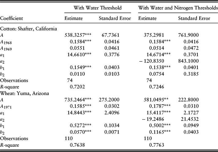
The empirical validity of the threshold factor idea is readily seen for the case of irrigation water for crop production in the desert Southwest region of the United States. During the late 1960s and early 1970s, Hexem and Heady (Reference Hexem and Heady1978) in collaboration with numerous agronomists and irrigation specialists conducted extensive field experiments involving crop (corn, corn silage, wheat, cotton, and sugar beets) response to varying irrigation water and nitrogen fertilization rates at 13 different agricultural experiment stations in Arizona, California, Colorado, Kansas, and Texas. In all, this massive project resulted in 52 distinct data sets (Hexem, Heady, and Caglar, Reference Hexem, Heady and Caglar1974). Characteristic of Heady's voluminous agricultural production function work, he and his coauthors estimated parameters for alternative quadratic polynomial and 1/2 and 3/2 power (quasi-polynomial) functional forms to the data.
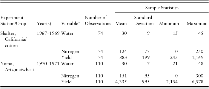
For purposes of this study, we fit two different variants of a Stone-Geary model to two of the Hexem-Heady desert Southwest data sets—cotton at Shafter, California, and wheat at Yuma (Valley), Arizona. In both cases, we took advantage of pooling multiple year data sets as the crop, experimental design, and experimental site was the same across time (see Table 1). Yearly dummies were included to capture otherwise unaccounted for differences between years (A 1968 and A 1969 for cotton at Shafter; A 1971 for wheat at Yuma). Of importance for our purpose—ascertaining the threshold level of water that is essential for positive yield—is the fact that the total water applied included preplant irrigation water applied and any rainfall in excess of one-quarter of an inch per occurrence during the growing season.
Table 1. Descriptive Statistics of Variables

a Water is measured in acre-inches, and nitrogen is measured in pounds per acre. Cotton yield is measured in pounds of lint per acre, and wheat yield is measured in pounds of wheat per acre. Because the Stone-Geary production function requires nonzero values for inputs, 1 was added to all nitrogen values in the estimations.
We used nonlinear least squares estimation, given that the Stone-Geary model is nonlinear in parameters. Columns 2 and 3 of Table 2 (water threshold only) are results of particular interest in demonstrating the viability of the Stone-Geary model in capturing the threshold input phenomenon. The empirical results are encouraging. Both base-year A-coefficient estimates are positive and statistically significant at the 1% level. All of the individual factor exponent estimates (bi) have the expected positive signs, and all have magnitudes in the required 0 < bi < 1 range for diminishing marginal productivity. Further, the 0 < b 1 + b 2 < 1 restriction for strict concavity for the two-variable-factor, short-run model is met. Three of the four exponent coefficient estimates are significant at the 1% level (the exception being the b 2 coefficient [nitrogen] for cotton at Shafter). Finally, and most important for demonstrating the empirical viability of the threshold factor idea, both a 1 estimates are positive and strongly significant (at the 1% level).
Table 2. Nonlinear Least Squares Estimates of Stone-Geary Production Functions
Notes: Asterisks (*, **, and ***) indicate significance at the 10%, 5%, and 1% levels, respectively. The complete empirical model for the Stone-Geary with two thresholds for cotton at Shafter, California, is y = Ae A 1968D1968e A 1969D1969(x 1 − a 1)b 1(x 2 − a 2)b 2, where D 1968 is a dummy variable for the year 1968, D 1969 is a dummy variable for the year 1969, x 1 is quantity of water, and x 2 is quantity of applied nitrogen. The empirical model for wheat is similarly defined.
The last two columns of Table 2 show results for a Stone-Geary specification with thresholds for both water and nitrogen. Initially, we did not consider a “threshold” for nitrogen in our modeling because in most fertilizer production-function applications one finds that a positive yield (a positive y-axis intercept) is obtained even when the fertilizer application rate is zero (a gratis threshold). This is attributable to naturally occurring plant-available nitrogen via agronomic nitrogen fixation prior to and during the course of the growing season. Nitrogen fixation, the conversion of N2 to plant-available N, is an ongoing process during the course of a growing season owing to microbial fixation (mineralization) in the soil and lightning and rain events (Allison, Reference Allison and Norman1955; Brady and Weil, Reference Brady and Weil2010; Stanford and Smith, Reference Stanford and Smith1972). The upshot is that applied (fertilizer) nitrogen represents only a partial accounting of the actual nitrogen that is available for plant growth during the course of a growing season, even when one includes, in measured N, preplant nitrogen estimates determined by soil testing.
This generalization of the Stone-Geary specification for firm-level production function modeling provides a way to parsimoniously deal with the unaccounted for (unmeasured/gratis) portion of an input. What one would hypothesize in such instances is that the threshold coefficient would have a negative rather than positive sign. As expected, that is what we found (see last two columns of Table 2). In both applications, the nitrogen threshold coefficient, a 2, is negative, although not significant. The fact that the gratis threshold for N is not significant is not particularly troubling. Although some N (specifically N that is mineralized during the course of the growing season) is unaccounted for in measured N, it is probably in most instances not a relatively great amount.
We believe these results provide compelling evidence that a threshold level of water necessary for positive yield clearly exists, at least in the desert Southwest—somewhere in the neighborhood of 15 acre-inches in our applications. It is our hypothesis that if our Stone-Geary model were fitted to other agricultural (and for that matter nonagricultural) production data sets, empirical evidence would mount for the threshold factor idea needing to be an important consideration for improved production function modeling for many, if not most, applications.
4. Summary and Conclusions
This article proposes and explores the implications of the Stone-Geary utility function as a production function model. The allowance for the possibility of threshold factor levels is theoretically compelling. The empirical support for a threshold factor level for irrigation water for crop production in the desert Southwest region of the United States is encouraging. Our empirical results, although less convincingly so, also suggest the possibility of a gratis threshold for nitrogen.
Also, as demonstrated in the Appendix, a Stone-Geary production function gives rise to an easily tractable variable cost function with U-shaped average variable cost. This pedagogical advantage enables a coherent presentation of production theory—consistency of input-side (factor demand) and output-side (product supply) analyses—without the unwieldy and unnecessary distractions of U-shaped marginal cost. It is our belief that the theoretical simplicity and empirical parsimony of the Stone-Geary model for accommodating factor thresholds for firm-level production modeling holds much promise for applied research and teaching in agricultural and resource economics.
Appendix
In the first section of this pedagogical appendix, we demonstrate the advantage of the Stone-Geary model for enabling a tractable variable cost function with U-shaped average variable cost from the underlying production function. The second section presents the Stone-Geary functional forms for conditional and ordinary factor demand and for product supply.
Tractable Variable Cost
Often in teaching principles and intermediate microeconomics, the (short-run) variable cost (VC) function is characterized as an elongated (stretched-out) backward S with associated U-shaped marginal cost (MC) and average variable cost (AVC) curves. Although we have no quarrel with such textbook presentations, we believe the suggestion (even if only implicit) that U-shaped MC is “typical” should be tempered. At a minimum, a caveat should be offered noting that most of the tractable production function models espoused by economists are not sufficiently flexible to enable U-shaped MC (Beattie and Almarri, Reference Beattie, Almarri and Beattie2011). Finally, to make matters worse, the mathematical specification of production function models consistent with U-shaped MC are sufficiently complex that getting from the production function to the VC function is generally intractable.
However, U-shaped AVC is necessary for development of the twin ideas of short-run shutdown and truncated supply for product prices less than minimum AVC as total revenue is insufficient to cover variable costs. An attractive feature of a Stone-Geary production function is that its associated AVC curve is U-shaped without the complication of U-shaped MC. For the single-variable-factor, short-run case and assuming perfect competition in the factor market, the variable-factor-cost equation is
 $$\begin{equation}
c = r_1 x_1 ,\end{equation}$$
$$\begin{equation}
c = r_1 x_1 ,\end{equation}$$where r 1 is the price of x 1. Taking the inverse of text equation (2), that is, finding x 1 = f − 1(y), and substituting into equation (A-1) gives the VC function, namely,
 $$\begin{equation}
{\rm VC} = r_1 \left( {a_1 + \alpha ^{ - {1 / {b_1 }}} y^{{1 /{b_1 }}} }\right),\end{equation}$$
$$\begin{equation}
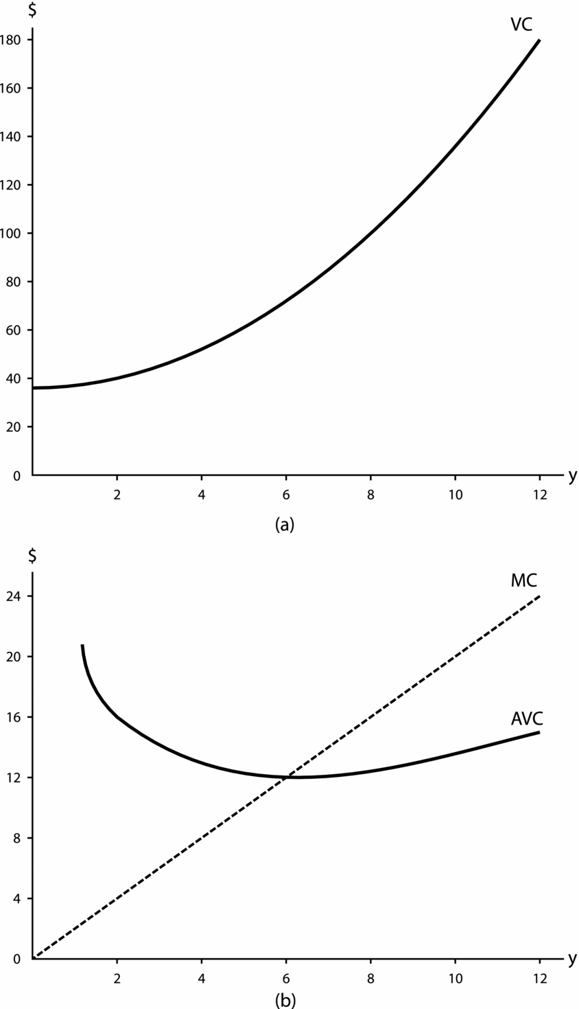
{\rm VC} = r_1 \left( {a_1 + \alpha ^{ - {1 / {b_1 }}} y^{{1 /{b_1 }}} }\right),\end{equation}$$which is plotted in Figure A1 (panel a) for the parameter values used for the plot of Figure 1 and assuming r 1 = 4.
Figure A1. Plot of Variable Cost (VC) and Marginal Cost (MC) and Average Variable Cost (AVC) for the Production Function, y = 2(x 1 − 9)1/2 for x 1 > 9
The derivative of equation (A-2) yields
 $$\begin{equation}
{\rm MC} = {{d{\rm VC}} / {dy = b_1^{ - 1} \alpha ^{{{ - 1} / {b_1 }}} r_1 y^{\left( {{1 / {b_1 }}}\right) - 1} = }}b_1^{ - 1} \alpha ^{{{ - 1} / {b_1 }}} r_1 y^{{{\left( {1 - b_1 }\right)} / {b_1 }}} .\end{equation}$$
$$\begin{equation}
{\rm MC} = {{d{\rm VC}} / {dy = b_1^{ - 1} \alpha ^{{{ - 1} / {b_1 }}} r_1 y^{\left( {{1 / {b_1 }}}\right) - 1} = }}b_1^{ - 1} \alpha ^{{{ - 1} / {b_1 }}} r_1 y^{{{\left( {1 - b_1 }\right)} / {b_1 }}} .\end{equation}$$
Notice that MC is monotonic, emanates from the origin, and increases either at an increasing, a constant, or a decreasing rate depending on whether  $b_1 < {1 / {2{\rm , } = }}{1 / {2{\rm , } > {1 / 2}}}$, respectively. In addition,
 $$\begin{equation}
{\rm AVC} = {\rm VC} \cdot y^{ - 1} = r_1 y^{ - 1} \left( {a_1 + \alpha ^{{{ - 1} / {b_1 }}} y^{{1 / {b_1 }}} }\right).\end{equation}$$
$$\begin{equation}
{\rm AVC} = {\rm VC} \cdot y^{ - 1} = r_1 y^{ - 1} \left( {a_1 + \alpha ^{{{ - 1} / {b_1 }}} y^{{1 / {b_1 }}} }\right).\end{equation}$$MC and AVC are shown in panel b of Figure A1. (Linearity of MC is an artifact of choosing b 1=1/2, giving rise to a quadratic VC function in equation A-4). What we observe in Figure A1 (panel b) is monotonically increasing MC intersecting a U-shaped AVC at its minimum—all that is needed for truncated product supply and short-run shutdown.
The results nicely and easily extend to multiple-variable-factor, short-run cases. The essential algebra for the two-variable-factor case follows:
 $$\begin{equation}
c = r_1 x_1 + r_2 x_2 ,\end{equation}$$
$$\begin{equation}
c = r_1 x_1 + r_2 x_2 ,\end{equation}$$the factor cost equation;
 $$\begin{equation}
y = A\left( {x_1 - a_1 }\right)^{b_1 } x_2^{b_2 } ,\end{equation}$$
$$\begin{equation}
y = A\left( {x_1 - a_1 }\right)^{b_1 } x_2^{b_2 } ,\end{equation}$$the short-run yield/production function (assuming a threshold for x 1 but not for x 2 and at least one suppressed fixed factor); and
 $$\begin{equation}
\frac{{f_1 }}{{f_2 }} = \frac{{r_1 }}{{r_2 }}\Rightarrow x_2 = \frac{{b_2 r_1 }}{{b_1 r_2 }}\left( {x_1 - a_1 }\right),\end{equation}$$
$$\begin{equation}
\frac{{f_1 }}{{f_2 }} = \frac{{r_1 }}{{r_2 }}\Rightarrow x_2 = \frac{{b_2 r_1 }}{{b_1 r_2 }}\left( {x_1 - a_1 }\right),\end{equation}$$the expansion path from the cost-minimization problem.
Substituting equation (A-7) into equations (A-5) and (A-6), respectively, to eliminate x 2 gives
 $$\begin{equation}
c = r_1 x_1 + r_2 \frac{{b_2 r_1 }}{{b_1 r_2 }}\left( {x_1 - a_1 }\right) = \left( {1 + \frac{{b_2 }}{{b_1 }}}\right)r_1 x_1 - a_1 \frac{{b_2 }}{{b_1 }}r_1\end{equation}$$
$$\begin{equation}
c = r_1 x_1 + r_2 \frac{{b_2 r_1 }}{{b_1 r_2 }}\left( {x_1 - a_1 }\right) = \left( {1 + \frac{{b_2 }}{{b_1 }}}\right)r_1 x_1 - a_1 \frac{{b_2 }}{{b_1 }}r_1\end{equation}$$and
 $$\begin{equation}
y = A\left( {x_1 - a_1 }\right)^{b_1 } \left( {\frac{{b_2 r_1 }}{{b_1 r_2 }}\left( {x_1 - a_1 }\right)}\right)^{b_2 } .\end{equation}$$
$$\begin{equation}
y = A\left( {x_1 - a_1 }\right)^{b_1 } \left( {\frac{{b_2 r_1 }}{{b_1 r_2 }}\left( {x_1 - a_1 }\right)}\right)^{b_2 } .\end{equation}$$Taking the inverse of equation (A-9) yields
 $$\begin{equation}
x_1 = y^{\frac{1}{{b_1 + b_2 }}} A^{ - \frac{1}{{b_1 + b_2 }}} \left( {\frac{{b_2 r_1 }}{{b_1 r_2 }}}\right)^{ - \frac{{b_2 }}{{b_1 + b_2 }}} + a_1 .\end{equation}$$
$$\begin{equation}
x_1 = y^{\frac{1}{{b_1 + b_2 }}} A^{ - \frac{1}{{b_1 + b_2 }}} \left( {\frac{{b_2 r_1 }}{{b_1 r_2 }}}\right)^{ - \frac{{b_2 }}{{b_1 + b_2 }}} + a_1 .\end{equation}$$Finally, substituting equation (A-10) into equation (A-8) obtains
 $$\begin{equation}
{\rm VC} = \left( {1 + \frac{{b_2 }}{{b_1 }}}\right)r_1 y^{\frac{1}{{b_1 + b_2 }}} A^{ - \frac{1}{{b_1 + b_2 }}} \left( {\frac{{b_2 r_1 }}{{b_1 r_2 }}}\right)^{ - \frac{{b_2 }}{{b_1 + b_2 }}} + a_1 \frac{{b_2 }}{{b_1 }}r_1 .\end{equation}$$
$$\begin{equation}
{\rm VC} = \left( {1 + \frac{{b_2 }}{{b_1 }}}\right)r_1 y^{\frac{1}{{b_1 + b_2 }}} A^{ - \frac{1}{{b_1 + b_2 }}} \left( {\frac{{b_2 r_1 }}{{b_1 r_2 }}}\right)^{ - \frac{{b_2 }}{{b_1 + b_2 }}} + a_1 \frac{{b_2 }}{{b_1 }}r_1 .\end{equation}$$Notice that if 0 < b 1 + b 2 < 1 as required for concavity of the production function, then the exponent on y will necessarily be >1 and VC will increase at an increasing rate. Also notice that VC has a positive $-axis intercept at a 1b −11b 2r 1.
Before considering MC and AVC, simplify equation (A-7) by letting  $A = \sqrt 8$, a 1 = 9, and $b_1 = b_2 = {1 / 4}$. Doing so gives
 $$\begin{equation}
{\rm VC} = (1/4)r_1^{1/2} r_2^{1/2} y^2 + 9r_1 .\end{equation}$$
$$\begin{equation}
{\rm VC} = (1/4)r_1^{1/2} r_2^{1/2} y^2 + 9r_1 .\end{equation}$$Letting r 1 = r 2 = 4, equation (A-12) simplifies to
 $$\begin{equation}
{\rm VC} = 36 + y^2 .\end{equation}$$
$$\begin{equation}
{\rm VC} = 36 + y^2 .\end{equation}$$Having purposefully selected parameter values different from those chosen for graphing the single-variable-factor case in Figure A1 results in the same VC, MC, and AVC as obtained previously. So, Figure A1 suffices.
We should note that one could obtain a like result (U-shaped AVC) that is similarly quite tractable by simply adding a negative constant term to a quadratic production function or, as we did in an earlier version of this article, adding a single constant term to the Cobb-Douglas. The problem with simply adding a single constant term to either a quadratic or Cobb-Douglas is that what one ends up with is a hodgepodge threshold effect that somehow applies across the board to all the inputs. The Stone-Geary formulation is preferable in that it enables us to sort out the threshold effect(s) and properly attribute it (them) to the appropriate factor(s). Indeed, as demonstrated in the empirical applications in the main text, we see that “thresholds” for some factors may in fact not be thresholds at all, but rather gratis thresholds or less than fully accounted for input effects. Certainly, for some (perhaps most) inputs, we might correctly presume no threshold effect at all. A single additive constant term unnaturally and undesirably muddles all such effects together.
Stone-Geary Factor Demand and Product Supply Functions
Assume two variable factors—both with threshold possibilities—and one fixed factor as given in text equation (1):
 $$\begin{equation}
y = \left\{ {\begin{array}{*{20}c}
0 & {{\rm for}\,x_1 \le a_1 \,{\rm or}\,x_2 \le a_2 } \\
{A(x_1 - a_1 )^{b_1 } (x_2 - a_2 )^{b_2 } x_3^{b_3 } } & {{\rm otherwise.}} \\
\end{array}}\right.\end{equation}$$
$$\begin{equation}
y = \left\{ {\begin{array}{*{20}c}
0 & {{\rm for}\,x_1 \le a_1 \,{\rm or}\,x_2 \le a_2 } \\
{A(x_1 - a_1 )^{b_1 } (x_2 - a_2 )^{b_2 } x_3^{b_3 } } & {{\rm otherwise.}} \\
\end{array}}\right.\end{equation}$$The conditional (cost-minimizing) factor demand functions are as follows:
 $$\begin{eqnarray}
x_1^c = A^{{{ - 1} / {(b_1 + b_2 }})} b_1^{{{b_2 } / {(b_1 + b_2 )}}} b_2^{{{ - b_2 } / {(b_1 + b_2 )}}} r_1^{{{ - b_2 } / {(b_1 + b_2 )}}} r_2^{{{b_2 } / {(b_1 + b_2 )}}} x_3^{{{ - b_3 } / {(b_1 + b_2 )}}} y^{{1 / {(b_1 + b_2 )}}}+ a_1\nonumber\\ \end{eqnarray}$$
$$\begin{eqnarray}
x_1^c = A^{{{ - 1} / {(b_1 + b_2 }})} b_1^{{{b_2 } / {(b_1 + b_2 )}}} b_2^{{{ - b_2 } / {(b_1 + b_2 )}}} r_1^{{{ - b_2 } / {(b_1 + b_2 )}}} r_2^{{{b_2 } / {(b_1 + b_2 )}}} x_3^{{{ - b_3 } / {(b_1 + b_2 )}}} y^{{1 / {(b_1 + b_2 )}}}+ a_1\nonumber\\ \end{eqnarray}$$ $$\begin{eqnarray}
x_2^c = A^{{ - 1}/{(b_1 + b_2 )}} b_1^{{{ - b_1 }/ {(b_1 + b_2 )}}} b_2^{{{b_1 }/{(b_1 + b_2 )}}} r_1^{{{b_1 }/{(b_1 + b_2 )}}} r_2^{{{ - b_1 }/{(b_1 + b_2 )}}} x_3^{{{ - b_3 }/{(b_1 + b_2 )}}} y^{{{1}/{(b_1 + b_2 )}}} + a_2 .\nonumber\\
\end{eqnarray}$$
$$\begin{eqnarray}
x_2^c = A^{{ - 1}/{(b_1 + b_2 )}} b_1^{{{ - b_1 }/ {(b_1 + b_2 )}}} b_2^{{{b_1 }/{(b_1 + b_2 )}}} r_1^{{{b_1 }/{(b_1 + b_2 )}}} r_2^{{{ - b_1 }/{(b_1 + b_2 )}}} x_3^{{{ - b_3 }/{(b_1 + b_2 )}}} y^{{{1}/{(b_1 + b_2 )}}} + a_2 .\nonumber\\
\end{eqnarray}$$Ordinary (profit-maximizing) factor demand and product supply functions are the following:
 $$\begin{equation}
x_1^* = A^{{{ - 1} / \alpha }} b_1^{{{(b_2 - 1)} / \alpha }} b_2^{{{ - b_2 } / \alpha }} r_1^{(1{{ - b_2 )} / \alpha }} r_2^{{{b_2 } / \alpha }} p^{{{ - 1} / \alpha }} x_3^{{{ - b_3 } / \alpha }} + a_1\end{equation}$$
$$\begin{equation}
x_1^* = A^{{{ - 1} / \alpha }} b_1^{{{(b_2 - 1)} / \alpha }} b_2^{{{ - b_2 } / \alpha }} r_1^{(1{{ - b_2 )} / \alpha }} r_2^{{{b_2 } / \alpha }} p^{{{ - 1} / \alpha }} x_3^{{{ - b_3 } / \alpha }} + a_1\end{equation}$$ $$\begin{equation}
x_2^* = A^{{{ - 1} / \alpha }} b_1^{{{ - b_1 } / \alpha }} b_2^{{{(b_1 - 1)} / \alpha }} r_1^{{{b_1 } / \alpha }} r_2^{{{(1 - b_1 )} / \alpha }} p^{{{ - 1} / \alpha }} x_3^{{{ - b_3 } / \alpha }} + a_2\end{equation}$$
$$\begin{equation}
x_2^* = A^{{{ - 1} / \alpha }} b_1^{{{ - b_1 } / \alpha }} b_2^{{{(b_1 - 1)} / \alpha }} r_1^{{{b_1 } / \alpha }} r_2^{{{(1 - b_1 )} / \alpha }} p^{{{ - 1} / \alpha }} x_3^{{{ - b_3 } / \alpha }} + a_2\end{equation}$$ $$\begin{equation}
y^* = A^{{{ - 1} / \alpha }} b_1^{{{ - 1} / \alpha }} b_2^{{{ - 1} / \alpha }} r_1^{{{b_1 } / \alpha }} r_2^{{{b_2 } / \alpha }} p^{{{ - (b_1 + b_2 )} / \alpha }} x_3^{{{ - b_3 } / \alpha }} ,\end{equation}$$
$$\begin{equation}
y^* = A^{{{ - 1} / \alpha }} b_1^{{{ - 1} / \alpha }} b_2^{{{ - 1} / \alpha }} r_1^{{{b_1 } / \alpha }} r_2^{{{b_2 } / \alpha }} p^{{{ - (b_1 + b_2 )} / \alpha }} x_3^{{{ - b_3 } / \alpha }} ,\end{equation}$$Given strict quasi-concavity (b 1 + b 2 > 0) for conditional factor demand and strict concavity (0 < b 1 + b 2 < 1) for ordinary factor demand and product supply, it is easily confirmed that the previous functions satisfy the usual expected homogeneity and comparative static properties.
As discussed in the previous section, because the Stone-Geary model affords U-shaped AVC, the product supply function in equation (A-19) does not hold for all r 1, r 2, p > 0. That is, the supply function is truncated where product price is less than minimum AVC as net returns exclusive of fixed cost (TR – VC) would be negative. The algebra for establishing the truncation point in general is onerous, but quite manageable if one chooses convenient numerical values for the production function parameters (A, a 1, a 2, b 1, b 2) and the fixed factor x 3 level. Using the same numerical values for those parameters as previously, that is,  $A = \sqrt 8 ,$a 1 = 9, a 2 = 0, $b_1 = b_2 = {1 / 4},$ and setting x 3 = 1, the truncation point for equation (A-19) is
 $$\begin{equation}
p \ge 3r_1^{3/4} r_2^{1/4} .\end{equation}$$
$$\begin{equation}
p \ge 3r_1^{3/4} r_2^{1/4} .\end{equation}$$Similarly, the ordinary factor demand curve truncation points for x*1 and x*2 given the same production function parameter values and fixed factor level as previously are easily established by solving equation (A-20) for the upper-bound r 1 and r 2 level, respectively.


 Open access