


1. Introduction
The exclusiveness of artificial microswimmers in harnessing energy from the surrounding fluid and converting it to useful mechanical energy for propulsion has made them suitable for a wide range of potential applications that include, but are not limited to, targeted drug delivery (Wang & Gao Reference Wang and Gao2012), disease diagnosis (Chałupniak, Morales-Narváez & Merkoçi Reference Chałupniak, Morales-Narváez and Merkoçi2015), environmental remediation (Li et al. Reference Li, Singh, Sattayasamitsathit, Orozco, Kaufmann, Dong, Gao, Jurado-Sanchez, Fedorak and Wang2014) and photothermal therapy (Choi et al. Reference Choi, Lee, Kim and Hahn2018). These microswimmers often take the form of micron-sized colloidal particles, widely known as Janus particles, which have asymmetric properties of their two faces. This asymmetric distribution of transport characteristics essentially triggers self-generated chemical, electrical, optical or thermal gradients (Paxton et al. Reference Paxton, Sundararajan, Mallouk and Sen2006; Howse et al. Reference Howse, Jones, Ryan, Gough, Vafabakhsh and Golestanian2007; Qian et al. Reference Qian, Montiel, Bregulla, Cichos and Yang2013; Jiang, Yoshinaga & Sano Reference Jiang, Yoshinaga and Sano2010; Lozano et al. Reference Lozano, Ten Hagen, Löwen and Bechinger2016), leading to intriguing propulsion characteristics despite the absence of any external forcing.
Among the different propulsion mechanisms, the chemical decomposition of hydrogen peroxide as a fuel source has been extensively studied in the literature (Paxton et al. Reference Paxton, Kistler, Olmeda, Sen, St. Angelo, Cao, Mallouk, Lammert and Crespi2004, Reference Paxton, Sundararajan, Mallouk and Sen2006; Gibbs & Zhao Reference Gibbs and Zhao2009; Wang et al. Reference Wang, Li, Li, Zhang and Sun2015; Poddar, Bandopadhyay & Chakraborty Reference Poddar, Bandopadhyay and Chakraborty2019a). However, its use in biomedical applications is limited due to its toxicity and the requirement of continuous supply of the same in the environment. Fuel-free locomotion can, however, be realized by localized heating of a metallic cap engendering a temperature gradient, which causes a directed self-thermophoretic locomotion (Jiang et al. Reference Jiang, Yoshinaga and Sano2010). The heating can be accomplished by different external stimuli such as illumination by laser beams (Jiang et al. Reference Jiang, Yoshinaga and Sano2010; Qian et al. Reference Qian, Montiel, Bregulla, Cichos and Yang2013; Bregulla, Yang & Cichos Reference Bregulla, Yang and Cichos2014; Ilic et al. Reference Ilic, Kaminer, Lahini, Buljan and Soljacic2016) or employing an alternating magnetic field (Baraban et al. Reference Baraban, Streubel, Makarov, Han, Karnaushenko, Schmidt and Cuniberti2013). Opto-thermal steering of the micromotor can also be performed by layering the two faces with different light-absorbing materials (Ilic et al. Reference Ilic, Kaminer, Lahini, Buljan and Soljacic2016). This coating pattern renders the local temperature gradient bidirectional, and selective lighting can result in a greater degree of control over the autonomous movement. Recently, a rotating electric field has also been employed to enhance the self-generated motion due to intrinsic thermophoresis (Chen, Yang & Jiang Reference Chen, Yang and Jiang2018). In addition, thermal modulation of microscale transport had been found advantageous in diverse aspects of lab-on-a-chip applications, e.g. drop manipulation (Das et al. Reference Das, Mandal, Som and Chakraborty2017; Das & Chakraborty Reference Das and Chakraborty2018; Das, Mandal & Chakraborty Reference Das, Mandal and Chakraborty2018), electrothermal flows (Kunti et al. Reference Kunti, Dhar, Bhattacharya and Chakraborty2018, Reference Kunti, Agarwal, Bhattacharya, Maiti and Chakraborty2019) and capillary transport (Chaudhury & Chakraborty Reference Chaudhury and Chakraborty2015; Bandopadhyay & Chakraborty Reference Bandopadhyay and Chakraborty2018).
Despite the obvious physical distinctions, thermally driven and solutally driven transport phenomena are commonly attributed to several conceptual similarities. In fact, it has been established that temperature and solute concentration fields as well as the fluid-flow patterns around an autophoretic particle in an unconfined fluid domain bear qualitative similarities, primarily due to analogies in the respective constitutive laws relating the fluxes with the gradients of the forcing parameter, and often a common framework of analysis may be adopted (Golestanian, Liverpool & Ajdari Reference Golestanian, Liverpool and Ajdari2007) to probe the pertinent implications. Exclusive geometrical and physical implications of a nearby wall, in addition, may influence the concerned aspects of particle locomotion to a significant extent. Inspired by the experimental evidence about the capability of a nearby wall in achieving precise navigation of a chemically active particle (Das et al. Reference Das, Garg, Campbell, Howse, Sen, Velegol, Golestanian and Ebbens2015), a host of studies has been aimed at analysing the motion of a self-diffusiophoretic micromotor near a solute-impermeable plane wall (Crowdy Reference Crowdy2013; Uspal et al. Reference Uspal, Popescu, Dietrich and Tasinkevych2015a; Ibrahim & Liverpool Reference Ibrahim and Liverpool2016; Mozaffari et al. Reference Mozaffari, Sharifi-Mood, Koplik and Maldarelli2016). However, taking cues from previously studied problems on passive particle thermophoresis near a wall (Chen Reference Chen1999, Reference Chen2000a,Reference Chenb), it can be realized that an isothermal wall is likely to bring in unique artefacts to the thermal modulations in active phoretic transport which by no means may be extrapolated trivially from other previously reported observations on diffusiophoretic transport in a wall-bounded flow. This may be attributed to the fact that the physical similitude of solute-impermeability condition for a diffusiophoresis problem leads to an equivalent adiabatic paradigm for a thermophoresis problem, which grossly deviates from an isothermal scenario.
In addition, contrasts in thermal conductivity between the particle and surrounding fluid are likely to result in key dynamical evolutions by virtue of altering the incipient thermo-hydrodynamic characteristics (Chen Reference Chen1999, Reference Chen2000a,Reference Chenb). While the implications of a nearby isothermal wall on the latter are presumably very complicated, the aspect of thermal conductivity gradient-driven transport of an active micromotor by itself has turned out to be an unaddressed phenomenon, even in an unbounded-flow domain (Jiang et al. Reference Jiang, Yoshinaga and Sano2010; Bickel, Majee & Würger Reference Bickel, Majee and Würger2013).
Here, we aim to unveil the physical consequences of a self-thermophoretic microswimmer adjacent to an isothermal plane wall; an aspect of active particle hydrodynamics that has hitherto remained unaddressed. The coupling between the thermal and the hydrodynamic field, mediated by kinematic constraints and thermal boundary conditions, is portrayed to be the key in dictating the unique dynamical evolution of the microswimmer trajectory under this purview. Instead of solving the full velocity profile of the fluid, we make use of the Lorentz reciprocal theorem (Happel & Brenner Reference Happel and Brenner1983) to evaluate the phoretic thrust experienced by the particle and employ the force-free conditions in obtaining the translational and rotation velocities of the swimmer. The exact solution of the energy equation is obtained by considering steady-state conditions and neglecting temperature distortion due to fluid advection. The results indicate that the thermal conductivity contrast between the particle and the surrounding fluid serves as a switching mechanism for the micromotor trajectories. With the interplay of the consequent forcing with the wall-induced thermophoresis, we further bring out multiple characteristics of near-wall swimming states that stand apart from the widely studied problem of self-diffusiophoresis in the proximity of an inert wall, and hold the key in opening up several novel applications featuring thermally activated control of active matter in a wall-bounded flow.
2. Mathematical formulation
We consider a micron-size Janus particle of thermal conductivity  $\varkappa _p$ in a fluid of thermal conductivity
  $\varkappa _f$. In typical cases, the particle is partially coated with gold (Au) or titanium-nitride (TiN), which absorbs light of specific frequency (Jiang et al. Reference Jiang, Yoshinaga and Sano2010; Ilic et al. Reference Ilic, Kaminer, Lahini, Buljan and Soljacic2016). This coating has been assumed to be axisymmetric about the director vector,
  $\boldsymbol {{d}}$, as shown in the figure 1(a). Upon irradiation of a laser beam, an asymmetric conversion to thermal energy takes place along the coated and uncoated faces of the particle. This has been modelled by incorporating a heat flux,
  $q''$ (in W m
 $^{-2}$), applied at the metal-coated half of the particle. This applied heat flux triggers a local temperature gradient around the particle, and, subsequently, a difference in osmotic pressure is created. Correspondingly, a slip flow is developed along the particle surface, and, while viewing from the laboratory frame, the particle is seen to propel itself. In an unbounded domain, the propulsion is directed along the director vector
  $\boldsymbol {{d}}$. This comprises the basics of an auto-thermophoretic microswimmer (Jiang et al. Reference Jiang, Yoshinaga and Sano2010; Bickel et al. Reference Bickel, Majee and Würger2013), albeit without any interactions with a nearby bounding wall. In the proximity to a constant temperature
  $(T_w)$ plane wall, this thermophoretic motion is likely to be altered significantly, which is the focal point of the subsequent analysis.
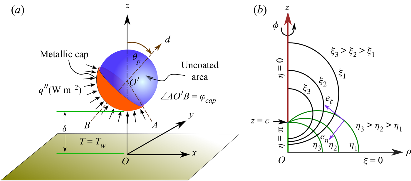
Figure 1. (a) Schematic of an auto-thermophoretic microswimmer near a constant temperature plane wall. The orange and blue faces of the particle represent the heat-absorbing metallic cap (hot) and uncoated (cold) areas on the micromotor surface, respectively. The angular orientation of the director vector  $\boldsymbol {{d}}$ is denoted by the angle
  $\theta _{p}$, measured in the clockwise direction from the positive
  $z$-axis. The coverage area of the metallic cap is represented by the angle
  $\varphi _{cap}$. The centre of the particle is at a distance of
  $\tilde {h}$ from the wall. (b) Schematic description of the bispherical coordinate used in the present study.
For theoretical depiction, we adopt the bispherical coordinate system  $(\xi , \eta , \phi )$ as shown in figure 1(b). This bispherical system is related to a corresponding cylindrical system
  $(\rho ,z,\phi )$ (with origin at the plane wall and the
  $z$-axis being directed normal to the wall and passing through the swimmer centre) as (Happel & Brenner Reference Happel and Brenner1983)
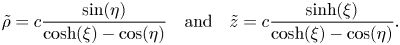 \begin{equation} \tilde{\rho}=c\frac{\sin(\eta)}{\cosh(\xi)-\cos(\eta)} \quad \text{and} \quad \tilde{z}=c\frac{\sinh(\xi)}{\cosh(\xi)-\cos(\eta)}. \end{equation}
Here,  $c$ is a positive scale factor,
  $\xi =0$ denotes the plane wall location and
  $\xi =\xi _0$ (
 $>$0) represents the spherical swimmer surface. The sphere has its centre situated at a height of
  $\tilde {z}=\tilde {h}=c \coth (\xi _0)$, and it has a radius of
  $a= c/\sinh (\xi _0)$. Thus, the smallest distance between the sphere surface and plane wall is
 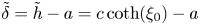 $\tilde {\delta }=\tilde {h}-a=c \coth (\xi _0)-a$.
2.1. Temperature distribution in and around the microswimmer
We neglect the flow-induced distortions in the temperature field and consider rapid diffusion of thermal energy, leading to a quasi-steady-state behaviour of the temperature distribution (Golestanian et al. Reference Golestanian, Liverpool and Ajdari2007). Hence, the energy equations in both the particle  $(p)$ and the surrounding fluid
  $(f)$ phases reduce to
 \begin{equation} \nabla^{2}T_{i} = 0,\quad i=p,f. \end{equation}
We leverage the fact that the laser-absorbing metallic cap, in many experimental scenarios, is only tens of nanometres in thickness  $(t_{cap})$, and that the particle radius
  $(a)$ lies in the range of microns (Jiang et al. Reference Jiang, Yoshinaga and Sano2010; Ilic et al. Reference Ilic, Kaminer, Lahini, Buljan and Soljacic2016). Moreover, the thermal conductivity of the cap is much larger than that of either the particle or the fluid. Thus, the condition
  $\varkappa _{cap}t_{cap} \gg \varkappa _p a$ is satisfied, and, following the earlier works (Jiang et al. Reference Jiang, Yoshinaga and Sano2010; Bickel et al. Reference Bickel, Majee and Würger2013), it may be judicious to assume the ‘thin-cap limit’. The thermal energy emitting from the laser-absorbing metallic cap causes a jump in the heat flux across the coated portion of the particle, while along the uncoated colder portion, a simple continuity of the heat flux is maintained. This is mathematically described by employing the following boundary condition at the particle surface:
 \begin{equation} \text{at} \ \xi=\xi_0, \quad -\varkappa_{f}(\boldsymbol{\nabla} T_{f})\boldsymbol{\cdot}\boldsymbol{{n}} + \varkappa_{p}(\boldsymbol{\nabla} T_{p})\boldsymbol{\cdot}\boldsymbol{{n}} = \mathcal{Q}(\boldsymbol{{n}}), \end{equation}
where  $\mathcal {Q}(\boldsymbol {{n}})$ is a piecewise function depicting the local rate of heat absorption per unit area of the particle surface, defined as
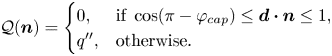 \begin{equation} \mathcal{Q}(\boldsymbol{{n}})=\begin{cases} 0, & \text{if} \ \cos(\pi- \varphi_{cap}) \le \boldsymbol{d} \boldsymbol{\cdot} \boldsymbol{n} \le 1,\\ q'', & \text{otherwise}. \end{cases} \end{equation}
The temperature is held fixed at the nearby flat wall  $(T_w)$. Without loss of generality, we set the wall temperature to zero with respect to a suitably chosen reference temperature, i.e.
 \begin{equation} \text{at} \ \ \xi=0,\quad T_w=0. \end{equation}
Further, the temperature gradient must vanish at large distances from the particle in the domain  $z > 0$.
In terms of the eigenfunctions in the bispherical coordinates, the temperature field in the surrounding fluid medium can be expressed as a solution of the Laplace equation (2.2) (Jeffery Reference Jeffery1912; Subramanian & Balasubramaniam Reference Subramanian and Balasubramaniam2001), as given below:
 \begin{align} T_{f} &= \sqrt{\cosh \xi - \cos\eta} \sum_{n=0}^{\infty} \sum_{m=0}^{\infty}[A_{n,m}\sinh(n+1/2)\xi +B_{n,m}\cosh(n+1/2)\xi] \nonumber\\ &\quad \times P_n^{m}(\cos\eta)\cos(m\phi + \gamma_m), \end{align}
with  $P_n^m$ denoting the associated Legendre polynomial of degree
  $n$ and order
  $m$; and
  $A_{n,m}$,
  $B_{n,m}$ and
  $\gamma_m$ are constant coefficients of degree n and order m. We emphasize the fundamental differences of the temperature distribution with that of the concentration profile of a closely related self-diffusiophoresis problem (Mozaffari et al. Reference Mozaffari, Sharifi-Mood, Koplik and Maldarelli2016). First, the boundary condition at
  $\xi =0$ (2.5) gives
  $B_{n,m}=0$. Thus, the outer region temperature profile reduces to
 \begin{equation} T_{f} = \sqrt{\cosh \xi - \cos\eta} \sum_{n=0}^{\infty} \sum_{m=0}^{\infty}A_{n,m}\sinh((n+1/2)\xi)P_n^{m}(\cos\eta)\cos(m\phi). \end{equation}
In stark contrast, the solute flux vanishes at the wall for the said self-diffusiophoresis problem, leading to the condition  $A_{n,m}=0$. The present solution exploits the bispherical coordinate system and renders the scalar (temperature or solute concentration) field easier to solve for a constant value of the scalar or its zero gradient at the wall. While tackling a wall boundary condition of Neumann type, i.e. the situation with specified, non-zero wall flux or, equivalently, a reactive wall with solute flux in self-diffusiophoresis, the present framework needs a few adjustments. In that case, the far-field natural boundary condition of zero scalar gradient has to be replaced with an essential boundary condition in terms of a specified scalar value. It is to be noted that this second category of problem is not the exact mathematical equivalent of the present work because the presence of the wall-adjacent micromotor breaks the equivalence that is observed in classical heat transfer problems with either specified wall flux or wall temperature in a semi-infinite domain (Carslaw & Jaeger Reference Carslaw and Jaeger1992).
In addition, contrary to the concentration profile for the corresponding self- diffusiophoresis problem, here, a complete description of the temperature profile demands a concurrent solution of the inner phase temperature distribution resulting from the redistribution of thermal energy inside the particle due to absorption of heat flux  $(q'')$ at the coated surface. Thus, the physical properties of the particle material also contribute to the final temperature distribution. In view of the boundedness of the temperature everywhere inside the particle, the solution of the thermal field turns out to be (Subramanian & Balasubramaniam Reference Subramanian and Balasubramaniam2001)
 \begin{equation} T_{p} = \sqrt{\cosh \xi - \cos\eta} \sum_{n=0}^{\infty} \sum_{m=0}^{\infty}d_{n,m} \textrm{e}^{-(n+1/2)\xi} P_n^{m}(\cos\eta)\cos(m\phi + \gamma_m), \end{equation}
 where  $d_{n,m}$ is a constant coefficient of degree n and order m and where the symmetry of the metallic cap about the
  $x$–
$x$– $z$ plane gives
  $\gamma _{n,m}=0$.
2.2. Hydrodynamics of near-wall self-thermophoresis
The selective absorption of heat along the swimmer surface creates an asymmetric distribution of temperature around the particle. Since the length scale  $(\tilde {l})$ of interaction between the particle and suspending fluid is much smaller than the microswimmer radius
  $(\tilde {l} \ll a)$, the flow pattern can be obtained following the boundary-layer theory (Anderson Reference Anderson1989; Golestanian et al. Reference Golestanian, Liverpool and Ajdari2007; Würger Reference Würger2010). The genesis of a tangential temperature gradient creates an osmotic pressure difference, which, in turn, drives a thermo-osmotic slip flow along the particle surface, given as (Anderson Reference Anderson1989; Kroy, Chakraborty & Cichos Reference Kroy, Chakraborty and Cichos2016)
 \begin{equation} \tilde{\boldsymbol{u}}^s=\mathcal{M} (\boldsymbol{I}-\boldsymbol{nn}) \boldsymbol{\cdot} \boldsymbol{\nabla} T_{S}, \end{equation}
where  $T_{S}$ denotes the particle surface temperature. Also,
  $\mathcal {M}$ denotes the thermophoretic mobility characterizing the particle–fluid interaction and is defined as
  $\mathcal {M} =-{\tilde {l}^2 \bar {\mathfrak {H} }}/{\mu T_0},$ where
  $\mu$ is the fluid viscosity,
  $\bar {\mathfrak {H}}$ is the characteristic value of the excess enthalpy and
  $T_0$ is the ambient temperature. In the present demonstrations, we consider a negative value of the excess enthalpy
  $(\bar {\mathfrak {H} }<0)$, which results in a fluid flow directed opposite to the temperature gradient in the surrounding fluid medium (Weinert & Braun Reference Weinert and Braun2008; Jiang et al. Reference Jiang, Yoshinaga and Sano2010). Since the fluid phase is initially immobile here, this thermo-osmotic flow from a co-moving frame is tantamount to a corresponding phoretic movement of the particle from a laboratory frame. It is noteworthy that in the case of passive diffusiophoresis, the mobility varies with solute concentration (Ault, Shin & Stone Reference Ault, Shin and Stone2019). Similarly, the temperature dependence of thermophoretic mobility may become significant for passive thermophoresis with nanometre-size particles (Braibanti, Vigolo & Piazza Reference Braibanti, Vigolo and Piazza2008). However, the works related to self-thermophoresis of micron-sized particles give substantial evidence that a theoretical treatment based on temperature-independent thermophoretic mobility is sufficient in this case (Jiang et al. Reference Jiang, Yoshinaga and Sano2010; Bregulla et al. Reference Bregulla, Yang and Cichos2014; Kroy et al. Reference Kroy, Chakraborty and Cichos2016). The analysis of the present work is in line with this observation in the latter scenario.
Subsequently, we incorporate a non-dimensionalization scheme, where different quantities are normalized by the following reference values: length  $\sim a$, heat flux
  $\sim q''$, thermal conductivity
  $\sim \varkappa _f$, temperature
  $\sim q'' a/ \varkappa _f$ and velocity
  $\sim - (\tilde {l}^2 \bar {\mathfrak {H} } q'' a/\mu T_0 \varkappa _f)$. Hereafter, we drop the ‘
  $\widetilde {\ }$ ’ symbol from various dimensional variables, and use the symbols
  $\boldsymbol {u}$,
  $\mathcal {K} (=\varkappa _p/\varkappa _f)$ and
  $\mathcal {T}$ in the analysis to denote dimensionless velocity, particle-to-fluid thermal conductivity ratio and dimensionless temperature, respectively.
In the creeping-flow limit (Happel & Brenner Reference Happel and Brenner1983), the flow field obeys the incompressibility condition and the Stokes equation as follows:
 \begin{equation} \boldsymbol{\nabla} \boldsymbol{\cdot} {\boldsymbol{u}}=0 \quad \text{and} \quad -\boldsymbol{\nabla} {p}+ \nabla^2 {\boldsymbol{u}}=0. \end{equation}
We analyse the hydrodynamic problem by observing the particle swimming from the laboratory reference frame. Thus, the flow velocity obeys the following boundary condition at the particle surface:
 \begin{equation} \boldsymbol{u}_s=\boldsymbol{V}+\boldsymbol{\varOmega} \times \boldsymbol{r}_{O'} + \boldsymbol{u}^s, \end{equation}
where  $\boldsymbol {V}$,
  $\boldsymbol {\varOmega }$ are the particle linear and rotational velocities, respectively, and
  $\boldsymbol{r}_{O'}$ is the radial distance vector from the particle center
  $O'$. On the other hand, a no-slip boundary condition is realized at the plane wall. The problem gets further simplified in view of the assumed axisymmetric coverage of the metal cap. This restricts the particle trajectory in the plane containing the wall normal and the symmetry axis of the swimmer. At the same time, the particle can rotate along an axis oriented orthogonal to both the plane wall normal and microswimmer director. Thus, the swimmer kinematics can be fully captured by focusing on
  $V_x$,
  $V_z$ and
  $\varOmega _y$. Additionally, due to its neutrally buoyant nature, the microswimmer will experience net-zero hydrodynamic force and torque conditions, i.e.
 \begin{equation} \boldsymbol{F}= \iint _{S_p} \boldsymbol{\sigma}\boldsymbol{\cdot} \boldsymbol{n}_{\boldsymbol{p}}\, \textrm{d}S=0 \quad \text{and} \quad \boldsymbol{C}= \iint_{S_p} \boldsymbol{r}_{O'} \times (\boldsymbol{\sigma}\boldsymbol{\cdot} \boldsymbol{n}_{\boldsymbol{p}})\, \textrm{d}S=0. \end{equation}
Here,  $S_p$ denotes the swimmer surface,
  $\boldsymbol {n}_{\boldsymbol {p}}$ is the unit normal to the swimmer surface and
  $\boldsymbol {\sigma }$ is the fluid stress tensor.
Similar to the earlier works on force-free microswimming (Lauga & Powers Reference Lauga and Powers2009; Montenegro-Johnson, Smith & Loghin Reference Montenegro-Johnson, Smith and Loghin2013; Qiu et al. Reference Qiu, Lee, Mark, Morozov, Münster, Mierka, Turek, Leshansky and Fischer2014; Datt et al. Reference Datt, Zhu, Elfring and Pak2015), we decompose the hydrodynamic problem into two subproblems: (i) the thrust problem that depicts fluid flow around a fixed microswimmer experiencing only a thermophoretic slip at the surface and (ii) the drag problem dealing with the rigid-body motion of a spherical particle where the hydrodynamic drag is only in action. Thus, the force and torque-free conditions can be written as
 \begin{equation} \boldsymbol{F}^{(Drag)}+\boldsymbol{F}^{(Thrust)}=0 \quad \mathrm{and} \quad \boldsymbol{C}^{(Drag)}+\boldsymbol{C}^{(Thrust)}=0, \ \text{respectively.} \end{equation}
The force and torque on a particle that is translating and rotating near a wall can be obtained by following the earlier works on a passive particle motion (Dean & O'Neill Reference Dean and O'Neill1963; O'Neill Reference O'Neill1964; Pasol et al. Reference Pasol, Chaoui, Yahiaoui and Feuillebois2005) and hence are not repeated here for the sake of brevity. Using the expressions for force and torque, determined for either unit velocity or rotation, as the resistance factors  $(\boldsymbol {\mathcal {R}}_T$,
  $\boldsymbol {\mathcal {R}}_C$ and
  $\boldsymbol {\mathcal {R}}_R$), we proceed to evaluate the drag force and torque for the unknown swimming velocity
  $(\boldsymbol {V})$ and rotation
  $(\boldsymbol {\varOmega })$, as given below
 \begin{align} \boldsymbol{F}^{(Drag)}&=\boldsymbol{\mathcal{R}}_T\boldsymbol{\cdot} \boldsymbol{V}+\boldsymbol{\mathcal{R}}_C^T\boldsymbol{\cdot} \boldsymbol{\varOmega}, \end{align}
 \begin{align} \boldsymbol{C}^{(Drag)}&=\boldsymbol{\mathcal{R}}_C\boldsymbol{\cdot} \boldsymbol{V}+\boldsymbol{\mathcal{R}}_R\boldsymbol{\cdot} \boldsymbol{\varOmega}. \end{align}
The task that remains is to determine the thrust force and torque on the microswimmer due to the self-thermophoretic actuation.
2.3. Employing the reciprocal theorem
To obtain the propulsive thrust on the microswimmer, we use the Lorentz reciprocal theorem applicable between two Stokes flows with similar geometry. It has the following general form (Happel & Brenner Reference Happel and Brenner1983):
 \begin{equation} \iint_{\partial S} \boldsymbol{{n}} \boldsymbol{\cdot} \boldsymbol{\sigma}' \boldsymbol{\cdot} \boldsymbol{u}''\,\textrm{d}S=\iint_{\partial S} \boldsymbol{{n}} \boldsymbol{\cdot} \boldsymbol{\sigma}'' \boldsymbol{\cdot} \boldsymbol{u'}\,\textrm{d}S. \end{equation}
Here ‘  $'$ ’ and ‘
  $''$ ’ superscripted variables correspond to those associated with the thrust problem and a complementary Stokes problem, respectively;
  $\partial S$ denotes the fluid confining boundary. Keeping in view of the no-slip condition for fluid velocity at the plane wall and decaying flow field at large distances from the microswimmer, we can simply use the swimmer surface
  $(S_p)$ in place of
  $\partial S$ in (2.15).
Since the kinematics of the problem indicate only non-zero components of velocities to be the translational velocities in the  $x$ and
  $z$ directions, and the rotational velocity in the
  $y$ direction, the calculation of thrust components demands the choice of the complementary Stokes problems as the following three fundamental problems related to the motion of a passively driven spherical particle near a wall:
(i) translation of the particle in the
 $+x$ direction with unit magnitude of the translational velocity;
(ii) translation of the particle in the
$+z$ direction with unit magnitude of the translational velocity; and(iii) rotation of the particle in the
$+y$ direction with unit magnitude of the rotational velocity.


A detailed treatment of these problems can be found from earlier works in the literature O'Neill (Reference O'Neill1964), Pasol et al. (Reference Pasol, Chaoui, Yahiaoui and Feuillebois2005) and Dean & O'Neill (Reference Dean and O'Neill1963), respectively.
Now utilizing the boundary condition on the surface of a fixed swimmer (2.11), the reciprocal relation (2.15) gives the thrust components on the swimmer as
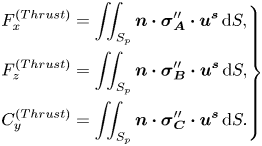 \begin{equation} \left.\begin{aligned} & F^{(Thrust)}_x=\iint_{S_p} \boldsymbol{n} \boldsymbol{\cdot} \boldsymbol{\sigma}_{\boldsymbol{A}}'' \boldsymbol{\cdot} \boldsymbol{u}^{\boldsymbol{s}}\,\textrm{d}S,\\ & F^{(Thrust)}_z=\iint_{S_p} \boldsymbol{n} \boldsymbol{\cdot} \boldsymbol{\sigma}_{\boldsymbol{B}}'' \boldsymbol{\cdot} \boldsymbol{u}^{\boldsymbol{s}}\,\textrm{d}S, \\ & C^{(Thrust)}_y=\iint_{S_p} \boldsymbol{n} \boldsymbol{\cdot} \boldsymbol{\sigma}_{\boldsymbol{C}}'' \boldsymbol{\cdot} \boldsymbol{u}^{\boldsymbol{s}}\,\textrm{d}S. \end{aligned}\right\} \end{equation}
Here,  $\boldsymbol {\sigma }_{\boldsymbol {A}}''$,
  $\boldsymbol {\sigma }_{\boldsymbol {B}}''$ and
  $\boldsymbol {\sigma }_{\boldsymbol {C}}''$ represent the fluid stress tensors corresponding to the complementary problems discussed above.
Although evaluated at the particle surface, the stress tensors in the force and torque expressions of (2.16) implicitly contain information about the flow boundary condition at the wall, i.e. the no-slip and no-penetration flow conditions. On the other hand, the surface-flow velocity embodies the effect of the specific thermal boundary condition at the wall due to the relation in (2.9). The thermal and the hydrodynamic field distributions are further interconnected through the kinematic constraints imposed by the wall and the constraints on force and torque (2.12).
3. Results and discussion
In the experimental realizations of the auto-thermophoresis (Jiang et al. Reference Jiang, Yoshinaga and Sano2010; Qian et al. Reference Qian, Montiel, Bregulla, Cichos and Yang2013; Chen et al. Reference Chen, Yang and Jiang2018), materials that have been used so far to fabricate a thermally asymmetric particle include microspheres made of ceramics, such as fused silica, and polymers, such as polystyrene, while the continuous fluid medium has been commonly taken as a mixture of water and glycerol. The typical thermal conductivities of these materials are given by: 1.3 W mK $^{-1}$ – fused silica (Touloukian et al. Reference Touloukian, Powell, Ho and Klemens1970), 0.13 W mK
 $^{-1}$ – polystyrene (Sombatsompop & Wood Reference Sombatsompop and Wood1997) and 0.54 W mK
 $^{-1}$ – water–glycerol mixture (Glycerine Producers’ Association 1963). Considering these materials, the thermal conductivity ratio is
  $\mathcal {K}=0.24$ (polystyrene–water) or
  $\mathcal {K}=2.407$ (silica–water). However, plenty of other materials have also been used to produce Janus particles with different functionalities (Hu et al. Reference Hu, Zhou, Sun, Fang and Wu2012) and are yet to be tested for their performance in auto-thermophoresis. It should be noted that, in the previous theoretical treatments of an unconfined self-thermophoresis (Jiang et al. Reference Jiang, Yoshinaga and Sano2010; Bickel et al. Reference Bickel, Majee and Würger2013), the parameter
  $\mathcal {K}$ has simply been chosen as 1, in view of the same order of magnitudes of the particle and fluid thermal conductivities. Thus, remaining consistent with the practical values and from the theoretical interest of capturing the key physical aspects of the thermal conductivity variation of the particle or fluid, we vary the thermal conductivity ratio
  $(\mathcal {K})$ from 0.1 to 10 during the illustration of results.
3.1. Temperature profile
In figure 2, we describe the effects of certain parameters on the resulting temperature profile due to self-thermophoresis. In the first case (figure 2a–c), the microswimmer director is leaning towards the wall, i.e. the cold portion is facing away from the isothermal wall  $(\theta _p=60^{\circ })$. Similarly, in figure 2(d–f), the inclination angle is
  $120^{\circ }$. The presence of the wall breaks the symmetry of the temperature distribution along the director axis.
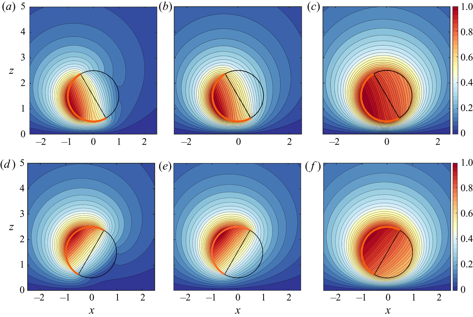
Figure 2. Spatial variation of the scaled temperature 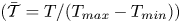 $(\bar {\mathcal {T}}=T/(T_{max}-T_{min}))$ in the
  $x$–
$x$– $z$ plane, both inside the microswimmer and in the surrounding fluid medium, for a fixed wall-swimmer distance of
  $\delta =0.5$ and a coverage angle of the metal coating
  $\varphi _{cap}=90^{\circ }$. The orientation angle (
 $\theta _{p}$) is
  $60^{\circ }$ in (a–c), while it is
  $120^{\circ }$ in (d–f). The thermal conductivity contrast has been varied as 0.1, 1 and 10 from left to right panels. The thick orange arc in each figure represents the metal-coated area of the surface.
  $(a,d)\, \mathcal {K} = 0.1, (b,e)\ \mathcal {K} = 1,\ (c,f)\ \mathcal {K} = 10.$
The surface temperature of the microswimmer  $\mathcal {T}_S$ is highly dependent on its distance from the wall, as shown in figures 3(a) and 3(c). In these figures, the variation of the angle
  $\theta_d$ denotes distance along the surface, measured clockwise from the director axis
  $\boldsymbol{d}$. Sensing a nearby low-temperature thermal obstacle, the micromotor surface temperature drops when the swimmer approaches the wall, irrespective of its inclination. Besides, the locations of the maximum and minimum temperatures on the particle surface vary with the distance. For both of the inclinations considered, the minimum temperature location shifts more towards the wall as the swimmer enters a wall-adjacent zone. In the former configuration, where the heated portion is closer to the wall, the maximum temperature location is shifted away from the wall as
  $\delta$ decreases. However, in the latter configuration, the maximum temperature location has only a negligible shift in the same direction. The above-mentioned maxima and minima locations of the surface temperature control the direction of surface slip flow, which, in the present case, is directed from a colder point to a hotter one on the surface.
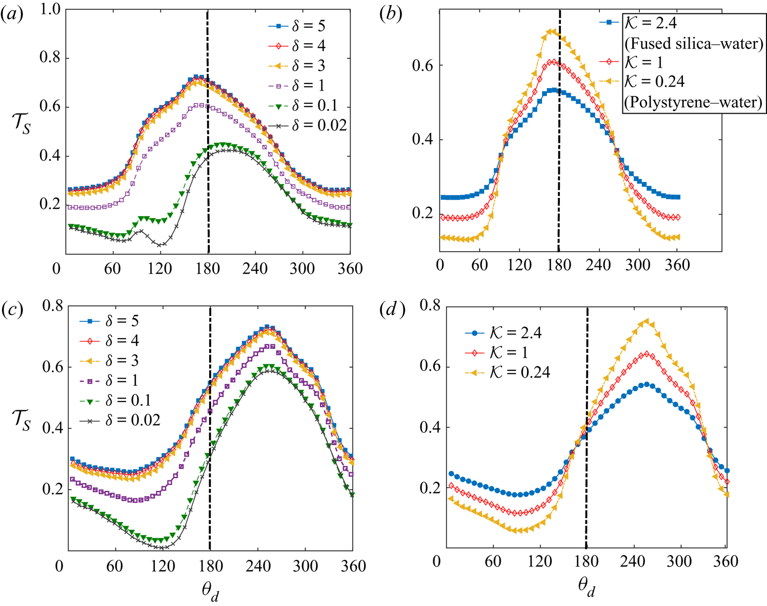
Figure 3. (a,b) Surface temperature  $(\mathcal {T}_S)$ variation along the surface for different wall distances and thermal conductivity ratios, respectively. Here, the angle
  $\theta _d$ is at the surface of the microswimmer, measured clockwise from the director axis
  $\boldsymbol {d}$. In (a), we have taken
  $\mathcal {K}=1$, while in (b)
  $\delta =1$. Other parameters are
  $\varphi _{cap} =90 ^{\circ }$ and
  $\theta _{p} =60 ^{\circ }$. In (c,d), similar variations are shown for a different inclination of
  $\theta _{p} = 120 ^{\circ }$. In each plot, the central vertical line provides visual assistance to identify the degree of asymmetry around the director axis,
  $\boldsymbol { d}$.
Comparing the temperature distributions in figures 2(a–c) or 2(d–f) we find that, as the particle material becomes relatively less thermally conductive than that of the surrounding fluid (i.e. a change of  $\mathcal {K}$ from 10 to 0.1), the hot-spot on the particle surface becomes progressively more localized owing to a poorer heat loss to the fluid. Such a physical situation can be imagined for metal-coated polymer spheres which bear distinct thermal properties, i.e. perfect conduction and perfect insulation, respectively. This ideal condition holds true only in the limit of
  $\varkappa _p \ll \varkappa _f$ or
  $\mathcal {K} \ll 1$. Consequently, such cases result in an enhanced temperature asymmetry around the micromotor. Along similar lines, in the above figures for
  $\mathcal {K}=0.1$ and 1, the metal-coated and uncoated halves show a vivid contrast in the isotherm contours coming out from the surface of the particle. On the other hand, with
  $\varkappa _{p}$ much higher than
  $\varkappa _{f}$, the hot area occupies a greater extent of the particle. However, in the limit of
  $\mathcal {K} \gg 1$, the particle becomes highly conducting and behaves almost as an isothermal body. This trend is reflected in figure 2(c,f) where the fluid-medium isotherms cut the surface almost parallel to it, and the insulating nature of the uncoated half is merely observed.
Strikingly, although the cap angle is low in figure 2, a high particle conductivity acts behind the trend of diminishing temperature heterogeneity around the particle, a phenomenon that is expected for the case of a very high metallic coverage, i.e.  $\varphi _{cap} \to 180^{\circ }$. For a generalized quantitative assessment of this observation, we define a temperature heterogeneity parameter
  $\mathcal {H}_T$ as
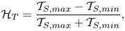 \begin{equation} \mathcal{H}_T=\frac{\mathcal{T}_{S,max}-\mathcal{T}_{S,min}}{\mathcal{T}_{S,max} +\mathcal{T}_{S,min}}, \end{equation}
representing a scaled difference between the maximum and minimum swimmer surface temperatures. This quantification is motivated from the deformation parameter frequently employed in drop deformation studies (Taylor Reference Taylor1966; Poddar et al. Reference Poddar, Mandal, Bandopadhyay and Chakraborty2018, Reference Poddar, Mandal, Bandopadhyay and Chakraborty2019b). To untangle the behaviour of the said heterogeneity from that due to non-axisymmetry around the wall normal, we have chosen  $\theta _p=180^{\circ }$ in figure 4. In figure 4(a), the effect of high thermal conductivity ratio
  $\mathcal {K}$ has been captured for different gaps from the wall. Here, a low coating coverage,
  $\varphi _{cap} =40 ^{\circ }$, has been chosen. On the other hand, figure 4(b) highlights the variations of
  $\mathcal {H}_T$ with high coating coverages,
  $\varphi _{cap}$, for different gaps from the wall. This case corresponds to a low conductivity ratio,
  $\mathcal {K}=0.1$. A comparison of the two figures re-affirms the common trend of decreasing heterogeneity for the two cases: (i)
  $\{ \mathcal {K} \gg 1 , \text { but low} \ \varphi _{cap} \}$ and (ii)
  $\{ \mathcal {K} \ll 1, \text { but high} \ \varphi _{cap} \}$. In addition, figure 4 suggests that, with decreasing gap between the microswimmer and the wall, the heterogeneous nature of surface temperature increases due to the tendency of reaching the limit of
  $\mathcal {T}_{S,min} \to \mathcal {T}_{wall}=0$. However, the impact of increasing
  $\mathcal {K}$ or
  $\varphi _{cap}$ on the temperature heterogeneity is asymptotically less pronounced at smaller gaps.
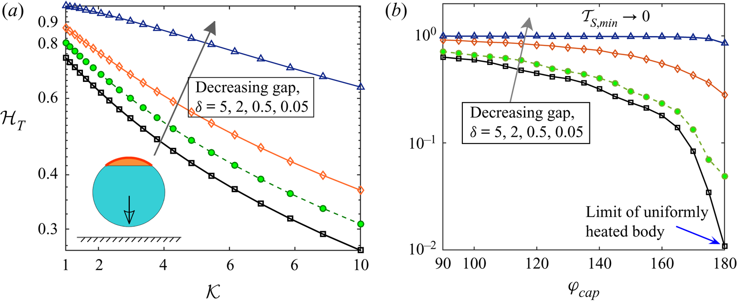
Figure 4. (a) Variation of temperature heterogeneity parameter,  $\mathcal {H}_T$, with high
  $\mathcal {K}$ for different gaps from the wall. Here, a low coating coverage,
  $\varphi _{cap} =40 ^{\circ }$, has been chosen. (a) Variation of
  $\mathcal {H}_T$ with high coverage angles,
  $\varphi _{cap}$, for different gaps from the wall. Here, a low conductivity ratio,
  $\mathcal {K}=0.1$, has been chosen. In both panels,
  $\theta _{p}=180^{\circ }$. The wall-swimmer configuration has been shown as an inset to the panel (a).
The effect of thermal conductivity contrast between the particle and fluid is also prominently extended in the fluid domain. For example, in the case of a highly conducting particle, the heated zone in the fluid almost surrounds the full circumference of the particle, as portrayed in figure 2(c,f).
The effects of contrasting thermal conductivities on the surface temperature profile have been demonstrated in figures 3(b) and 3(d) for inclinations  $60^{\circ }$ and
  $120^{\circ }$, respectively. We have chosen typical values of
  $\mathcal {K}$ for which the particle is more conductive than the fluid (
 $\mathcal {K}>1$) and vice versa (
 $\mathcal {K}<1$). With the hot surface facing the wall, the
  $\mathcal {K}>1$ condition causes a raise in the surface temperature before reaching
  $\theta \approx 155^ \circ$; thereafter, the temperature decays until
  $\theta \approx 325^ \circ$ and again raises beyond this location. Locations of these turnover points on the surface as well as the behaviour of temperature with changing
  $\mathcal {K}$ between these points are modified when the cold portion faces the wall.
3.2. Effect of thermal conductivity contrast in an unbounded flow
Before investigating the coupled interplay between the thermal conductivity contrast and the bounding wall on the microswimmer velocity, we delineate its behaviour in an unbounded domain. In an unbounded flow, the rotational component of the swimmer velocity does not exist since the wall-induced asymmetry in the temperature and flow field are absent in this case. The linear velocity magnitude 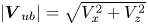 $|\boldsymbol {V}_{ub}|=\sqrt {V_x^2+V_z^2}$ depends only on the metallic cap coverage,
  $\varphi _{cap}$, and the thermal conductivity ratio,
  $\mathcal {K}$, as portrayed in figure 5(a). It is observed that the effect of
  $\varphi _{cap}$ on
  $|\boldsymbol {V}_{ub}|$ is symmetric about the
  $50\,\%$ coverage
  $(\varphi _{cap}=90^{\circ })$. On the other hand, the effect of increasing
  $\mathcal {K}$ is to decrease the velocity magnitude due to reduced temperature gradients.
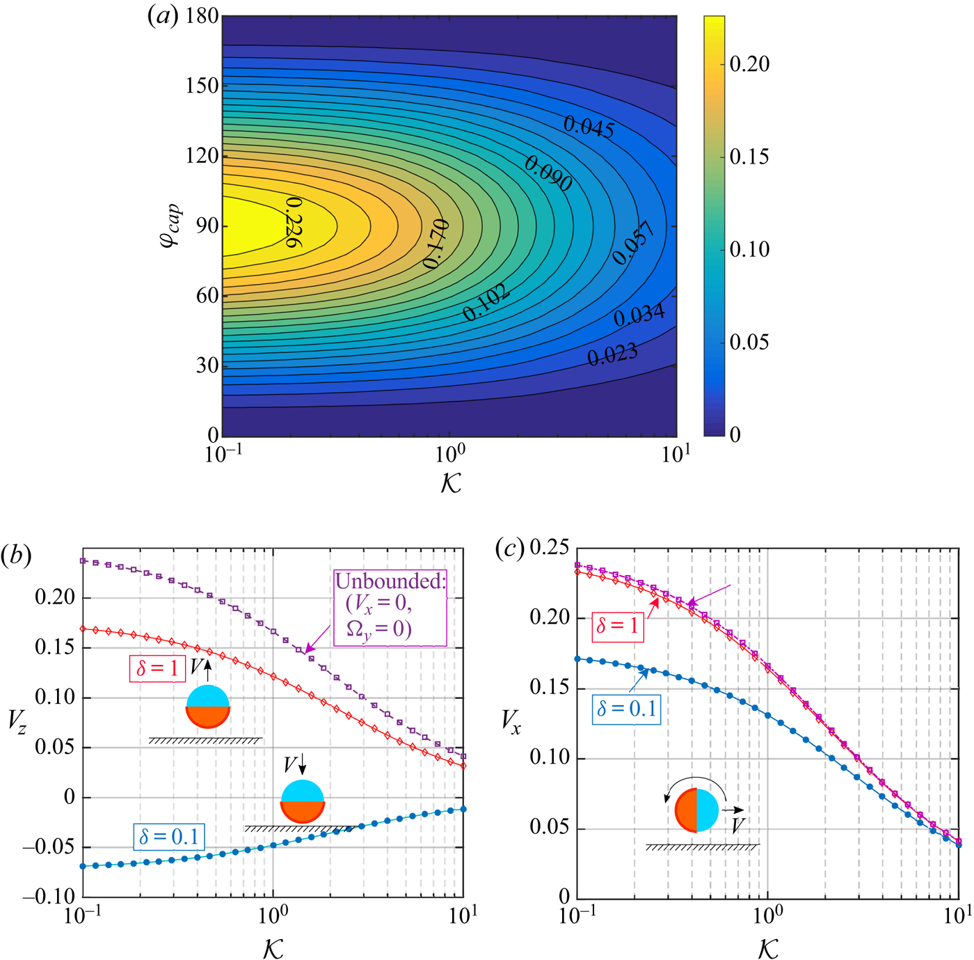
Figure 5. In (a), the unbounded swimming velocity magnitude  $|\boldsymbol {V}_{ub}|$ is shown in the
  $\mathcal {K}-\varphi _{cap}$ plane. In (b,c), the variations in velocity components (
 $V_z$ and
  $V_x$, respectively) with the thermal conductivity contrast (
 $\mathcal {K}$) are shown for both unbounded and near-wall scenarios. The orientation and velocity direction of the particle are shown schematically in each figure.
The wall-induced distortion of the temperature field weakens asymptotically and, beyond a certain height, the thermal boundary condition at the wall is likely to become inconsequential. A simultaneous decay in the hydrodynamic disturbance also takes place, tending towards a situation equivalent to that of an unbounded scenario. We quantify this distance with an effective separation distance,  $\delta _{ub}$, at which a velocity component of the microswimmer becomes
  $99\,\%$ of the unbounded velocity magnitude
  $|\boldsymbol {V}_{ub}|$. This effective distance is a function of the thermal and configurational parameters, i.e.
  $\delta _{ub}=\delta _{ub}(\mathcal {K},\theta _p,\varphi _{cap})$. As an example of this functional dependence, we show two reference configurations of the particle motion in figures 5(a) and 5(b), where either of the linear velocity component of the microswimmer exists in an unbounded domain. While in the first instance (figure 5b), the
  $\delta _{ub}$ for the vertical velocity component reduces from
  $\delta _{ub}=7.58$ for
  $\mathcal {K}=0.1$ to
  $\delta _{ub}=6.89$ for
  $\mathcal {K}=10$, in the second instance, (figure 5c) the
  $\delta _{ub}$ for the horizontal velocity component reduces from
  $\delta _{ub}=1.61$ for
  $\mathcal {K}=0.1$ to
  $\delta _{ub}=0.63$ for
  $\mathcal {K}=10$. The difference in the
  $\delta _{ub}$ for different velocity components indicates a contrasting nature of the wall effects in different flow directions.
3.3. Combined interplay of bounding wall and thermal conductivity contrast
In both the figures 6(a) and 6(b), the downward translation of the swimmer is intensified due to the presence of the wall, and, subsequently, it reaches an optimum (maximum magnitude) at a certain vertical distance  $(\delta _{opt})$. Away from the wall, this motion is retarded. When the coated surface faces the wall
  $(\theta _p=60^\circ )$,
  $V_z$ remains negative until a certain distance of
  $\delta _{cr} \approx 0.3$ from the wall; then it shows a trend of positive
  $V_z$. Finally, the swimmer gradually reaches a velocity that it would have attained if it were isolated. In the second configuration
  $(\theta _p=120^\circ )$, where the uncoated surface is nearer to the wall, the swimmer continues to translate downwards irrespective of the wall distance. For both the configurations, the location of
  $\delta _{opt}$ is shifted far from the wall, as the particle becomes increasingly more conductive (increasing
  $\mathcal {K}$). Such a consequence implies the coupled interplay between the particle-to-fluid thermal conductivity ratio and the wall distance in influencing the particle velocity.
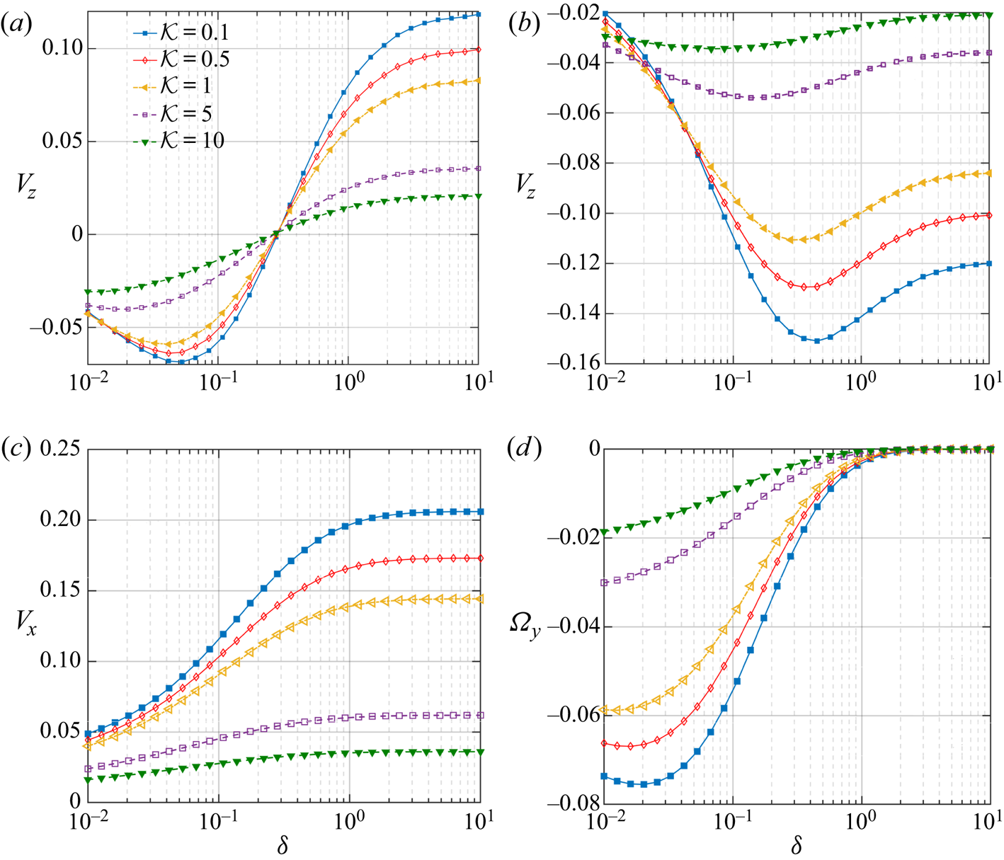
Figure 6. Variation of translational and rotational velocity components of the microswimmer with distance from the wall  $(\delta )$ and various thermal conductivity ratios
  $(\mathcal {K})$. The heated cap coverage is identically chosen as
  $\varphi _{cap} =90 ^{\circ }$ for all the cases. In (a,b),
  $\theta _{p} =60 ^{\circ }$ and
  $120\,^{\circ }$, respectively. Due to symmetry reasons, the (c) and (d) are applicable for both
  $\theta _{p}= 60 ^{\circ }$ or
  $120\,^{\circ }$.
The vertical translational velocity  $V_z$ can be calculated from the following reduced version of the general force-free relation (2.13):
 \begin{equation} V_z={-}F_z^{(Thrust)}/f_z^{T}, \end{equation}
where  $f_z^T$ is the resistance factor for translation in the
  $z$ direction. Thus, the velocity reversal in the
  $z$ direction can be explained solely from the behaviour of the vertical phoretic thrust, considering that the associated resistance factor,
  $f_z^T$, does not change its sign. As previously discussed, a variation in the swimmer-wall distance intervenes with the swimmer surface temperature distribution, and thereby its gradient along the surface is also affected. Because of this, the slip flow at the particle surface (2.9) is modified. Simultaneous to the distortions in the temperature field, the hydrodynamic stress distribution around the particle is also disturbed by the confining boundary. Both of these mechanisms work behind an altered thrust force experienced by the microswimmer (2.16).
Following the same figures, the thermal conductivity contrast  $(\mathcal {K})$ can neither shift the critical distance for the velocity reversal, nor can it alter the sign of velocity in both the swimmer inclinations considered. However, for a specific wall to swimmer distance
  $(\delta )$, the swimmer translates slower with escalating values of
  $\mathcal {K}$. While uncovering the associated physical mechanism, we refer to the attenuation of the asymmetry in temperature around the coated and uncoated faces of the microswimmer with high particle conductivity (see figure 2c,f), causing attenuation in the surface temperature gradient. This occurrence can be quantitatively visualized from the fact that in figure 3(b,d), with increasing
  $\mathcal {K}$, the maximum temperature falls, but the minimum temperature hikes, despite their corresponding locations on the surface being hardly affected. Hence, a weaker surface temperature gradient (i.e.
  $\mathcal {T}_{max}-\mathcal {T}_{min}$) is generated and, eventually, the surface flow is weakened. Accordingly, a diminishing surface traction strength on the swimmer surface results. It is to be noted that, in figure 6(b), very close to the wall
  $( \delta \lesssim 0.05)$, the variation in
  $V_z$ shows a non-monotonic dependence on the thermal conductivity contrast,
  $\mathcal {K}$. In the narrow gap region, strong hydrodynamic stresses build up, which are critically coupled with the flow modulations due to variations in the thermal conductivity. Accordingly, the thrust force varies non-monotonically with
  $\mathcal {K}$, as portrayed in figure 7.
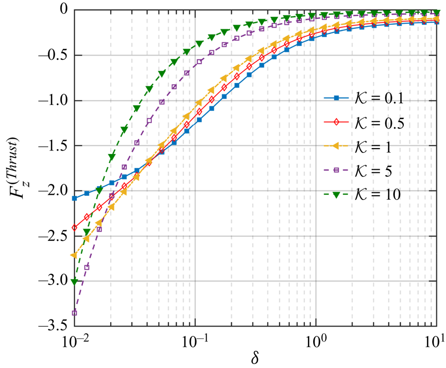
Figure 7. Variation of the vertical thermophoretic thrust  $(F_z^{(Thrust)})$ with
  $\delta$ and for different values of
  $\mathcal {K}$. The parameters are similar to figure 6(b).
In figure 6(c,d), we portray the variations in wall-parallel translational and rotational velocities with the parameters  $\delta$ and
  $\mathcal {K}$. The particle is slowed down as it approaches the wall, and it moves faster with lessened particle thermal conductivities. The near-wall rotation remains in the clockwise direction throughout, although the magnitude decays with strengthened particle thermal conductivity. While exploring other interesting facets of the velocity components, we have shown the variations in
  $V_x$ and
  $\varOmega _y$ in figures 8(a) and 8(b), respectively, for a different coverage angle of
  $\varphi _{cap} =140^{\circ }$ and inclination,
  $\theta _{p} =150 ^{\circ }$. As suggested by figure 8(a), with increasing distances from the wall, the horizontal migration velocity of the microswimmer also shows an increasing tendency. However, the swimmer is subsequently retarded beyond a specific separation height. Further, as the particle thermal conductivity reduces, the location of this maximum point shifts far from the wall. We also observe a change in the direction of the particle rotation from counterclockwise to clockwise at a fixed distance from the wall
  $(\delta \approx 0.11)$.
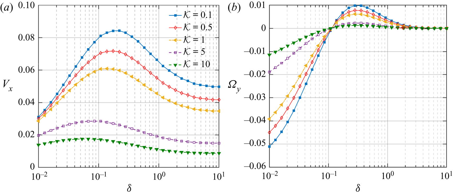
Figure 8. Variation of wall-parallel translational and rotational velocities of the microswimmer with distance from the wall  $(\delta )$ and different thermal conductivity ratios
  $(\mathcal {K})$. Other parameters are chosen as
  $\varphi _{cap} =140 ^{\circ }$ and
  $\theta _{p} =150 ^{\circ }$.
For gaining an insight into the physical origin of such behaviours, we first look into the expressions of  $V_x$ and
  $\varOmega _y$. Unlike the vertical velocity, the parallel rotation and translation velocities can only be obtained by solving a coupled system (2.13). This gives
  $V_x$ and
  $\varOmega _y$ in the following forms:
 \begin{equation} V_x=\dfrac{{F_x^{(Thrust)} f_{y}^R}- C_y^{(Thrust)} f_{x}^R }{f_{x}^Rf_{y}^T-f_{x}^T f_{y}^R} \quad \text{and} \quad \varOmega_y=\frac{C_y^{(Thrust)} f_{x}^T- F_x^{(Thrust)} f_{y}^T}{f_{x}^Rf_{y}^T-f_{x}^Tf_{y}^R}, \end{equation}
where different hydrodynamic resistance factors are defined as 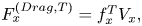 $F_{x}^{(Drag,T)}=f_{x}^TV_x,$
  $F_{x}^{(Drag,R)}=f_{x}^R\varOmega _y$,
  $C_{y}^{(Drag,T)}=f_{y}^T V_x$ and
  $C_{y}^{(Drag,R)}=f_{y}^R\varOmega _y$. It can be inferred from (3.3b) that the actual sign of the rotational velocity is a complex function of the hydrodynamic resistance factors as well as the thrust force and torque. From the previous investigations, it is known that these resistance factors increase in magnitude with a gradual descent of the particle towards the wall (Goldman, Cox & Brenner Reference Goldman, Cox and Brenner1967; Chaoui & Feuillebois Reference Chaoui and Feuillebois2003). Now, since the hydrodynamic resistance term in the denominator remains negative always (see figure 9), it is evident that the sign of
  $\varOmega _y$ is set by the relative importance of the phoretic torque (
 $C_y^{(Thrust)} f_{x}^T$) and the phoretic force
  $(F_x^{(Thrust)} f_{y}^T)$, adjusted by appropriate units. From a physical perspective, these two effects correspond to the counterclockwise torque due to the propulsive effects and the clockwise torque due to its forward movement
  $(+V_x)$, respectively. The counterclockwise torque is a net effect of the differently directed surface flows based on the locations of peak points in the surface temperature (a diagrammatic representation of a similar scenario has been provided later in figure 16d). The mechanism of the clockwise torque can be understood by considering the case when a lateral force causes a spherical particle to translate without any rotation parallel to a plane wall. The existence of confinement creates high velocity gradients in the lower half of the particle that faces the wall. In turn, the shear stress that the fluid exerts on the particle becomes much stronger in this region than that in the upper half away from the wall. This asymmetry in stress build-up exerts a torque on the particle. For translation along the
  $+x$ direction, this generated toque always acts in the clockwise direction, and the torque magnitude increases with a raise in
  $V_x$.
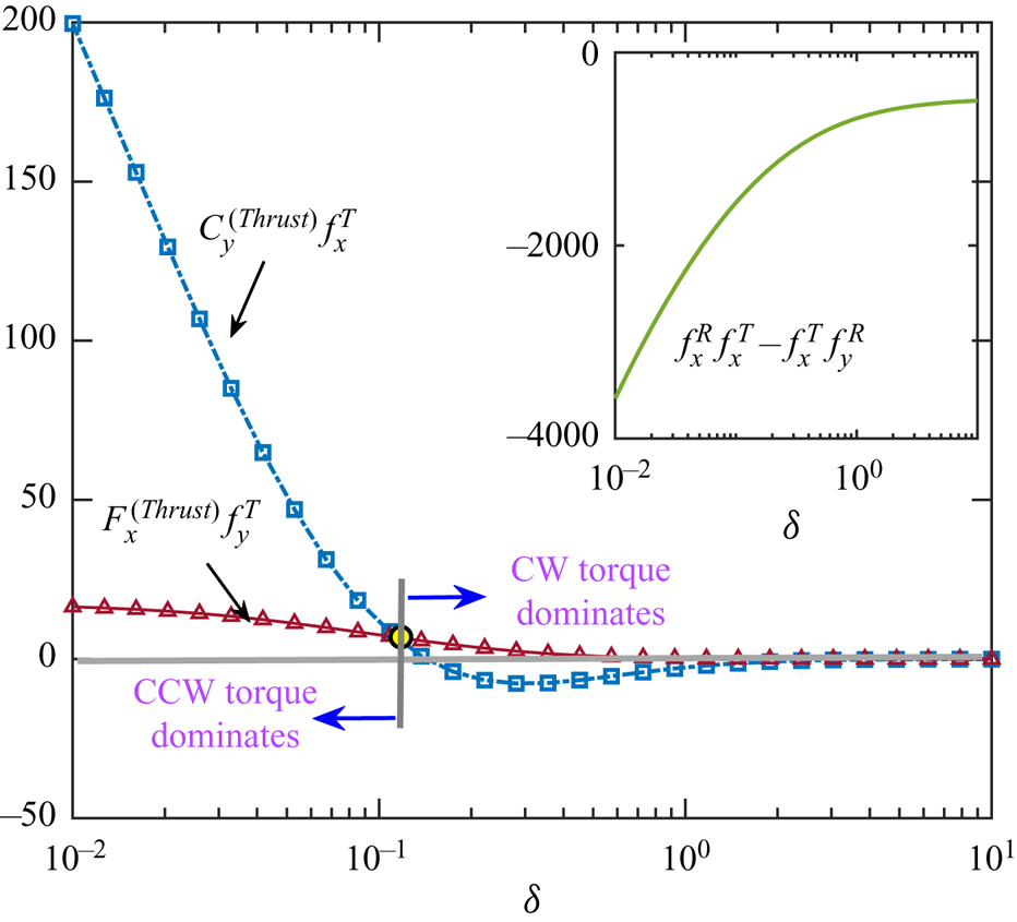
Figure 9. Detailed variation of different terms in (3.3b). The parameters are similar to figure 8(b). The yellow bubble signifies the location where 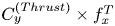 $C_y^{(Thrust)}\times f_{x}^T$ becomes smaller than
 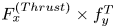 $F_x^{(Thrust)}\times f_{y}^T$.
Inspection of the temperature profiles at different distances from the wall reveals that the minimum temperature location shifts more towards the wall with a decreasing gap, while the maximum point remains almost unaffected. Subsequently, greater strength of the clockwise surface flow and an ensuing counterclockwise torque result. Also, as the micromotor approaches closer to the wall, it is subjected to the elevated hydrodynamic stresses because of near-wall velocity gradients. Such effects result in the relative dominance of the counterclockwise torque surpassing the opposing clockwise torque. Thus, at the reduced distances from the wall, we have a negative sign of  $\varOmega _y$. However, beyond a critical height, the effect of increasing
  $V_x$ (see figure 8a) becomes dominant and so does the corresponding clockwise torque.
It is exciting to note that the critical gap sizes  $(\delta _{cr})$ at which the particle switches its vertical swimming direction (figure 6a) and angular rotation (figure 8b) are independent of the conductivity ratio,
  $\mathcal {K}$. The physical origin of such behaviour can be perceived by investigating the way the factor
  $\mathcal {K}$ influences the thermophoretic thrust. Any characteristic shift in thrust force or torque has to be assisted by corresponding modulations in the thermophoretic slip flow around the particle. For a better understanding, we first appeal to figures 3(b) and 3(d) where it has been observed that the locations of the peaks of surface temperature,
  $\mathcal {T}_{S,max}$ and
  $\mathcal {T}_{S,min}$, remain unaltered with variations in
  $\mathcal {K}$. These peak locations are crucial in governing the fluid flow directions at the surface, as indicated by (2.9). As a consequence, the direction of surface flow will also remain unaltered with
  $\mathcal {K}$ owing to fixed peak temperature locations. This characteristic feature of surface flow is responsible for not altering the condition (i.e. the specific value of
  $\delta$) required for vanishing phoretic thrust force and torque.
3.4. Existence of fixed points
Here, we report the existence of fixed points in the vertical component of velocity of the self-thermophoretic microswimmer. It has been found that the critical gap size for the reversal of vertical motion,  $\delta _{cr}$, depends both on the metallic coating coverage,
  $\varphi _{cap}$, and the swimmer orientation,
  $\theta _p$, as depicted in figure 10(a). Conceptually similar fixed points were reported in the literature dealing with self-diffusiophoretic microswimmers near confinements (Uspal et al. Reference Uspal, Popescu, Dietrich and Tasinkevych2015a; Nasouri & Golestanian Reference Nasouri and Golestanian2020).
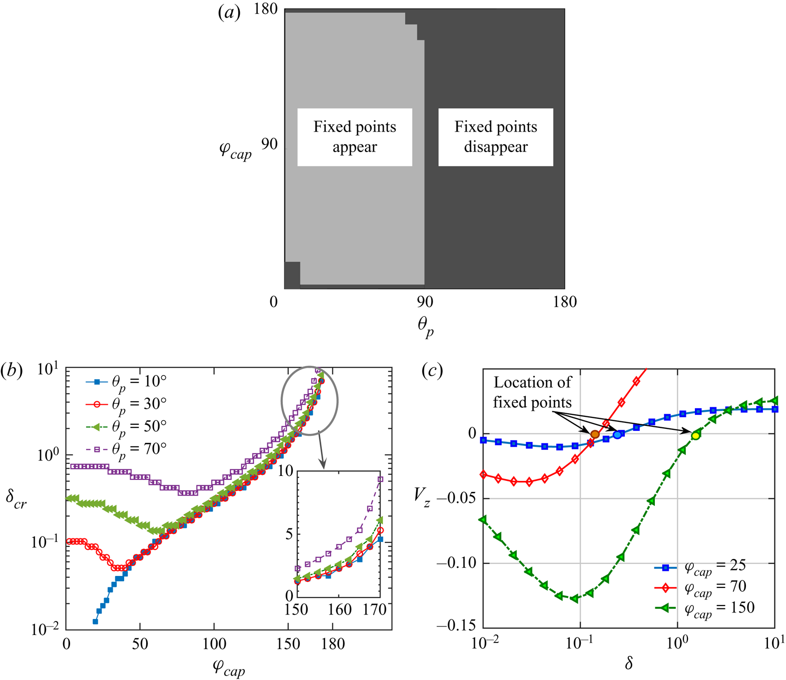
Figure 10. (a) Phase map demarcating the limits of metallic coating coverage,  $\varphi _{cap}$, and the swimmer orientation,
  $\theta _p$, for the existence of fixed points in the vertical component of velocity,
  $V_z$. (b) Critical gap size,
  $\delta _{cr}$, vs. the coating coverage,
  $\varphi _{cap}$, for different swimmer orientations,
  $\theta _p$. Data points have been obtained by searching in a grid of 50 equally spaced points (in log scale) for
  $\delta$ and with a linear increment of
  $2.5^{\circ }$ for
  $\varphi _{cap}$. (c) The vertical velocity,
  $V_z$, vs. gap thickness,
  $\delta$, for different coating coverages and
  $\theta _p=50^{\circ }$.
Figure 10(a) suggests that for  $\theta _p \ge 90^{\circ }$, the fixed points do not appear, while for
  $\theta _p < 90^{\circ }$, the fixed points appear even for very low extent of metallic coating. In addition, for low values of
  $\theta _p$, e.g. for
  $\theta _p \lesssim 10^{\circ }$, a minimum metallic coverage,
  $\varphi _{cap} \gtrsim 17.5 ^{\circ }$, is required for the fixed points to exist. However, for greater orientation angles,
  $10^{\circ } < \theta _p <90^{\circ }$, the fixed points appear even for a minimal coating extent of
  $\varphi _{cap} \gtrsim 2.5 ^{\circ }$. It is to be noted that the disappearance of fixed points below these minimum coating angles is due to the mathematical artefact that a minimum cutoff gap is required to be set while searching for the fixed points employing a numerical algorithm. The minimum cutoff gap has been presently chosen as
  $\delta =0.01$, while the same was chosen as
  $\delta =0.02$ in Uspal et al. (Reference Uspal, Popescu, Dietrich and Tasinkevych2015b). Similarly, the upper limit of
  $\delta$ during the numerical searching of fixed points has been chosen as
  $\delta =10$. The reader may refer to the work of Ishimoto & Gaffney (Reference Ishimoto and Gaffney2013) for the practicality behind choosing such a limiting value. This is the reason behind the vanishing fixed points in the common region near
  $\theta _p \to 90^{\circ }$ and
  $\varphi _{cap} \gtrsim 160^{\circ }$ (see the upper right corner of the grey half in figure 10a), indicating the probable fixed points beyond the highest gap considered here.
The variation of the critical gap size with the coating coverage has been highlighted in figure 10(b). The figure suggests a non-monotonic dependence of  $\delta _{cr}$ on
  $\varphi _{cap}$, especially when the orientation angle,
  $\theta _{p},$ is high. In these cases, the critical gap has a minimum value at a certain value of coating coverage for the respective orientation. Any shift from these coverage extents causes an increase in the critical gap magnitude. Figure 10(c) displays the location of fixed points for varying coating coverages on the
  $V_z$ vs.
  $\delta$ curves for a specific swimmer orientation,
  $\theta _p=50^{\circ }$. This behaviour was not reported concerning self-diffusiphoresis (Uspal et al. Reference Uspal, Popescu, Dietrich and Tasinkevych2015a). The said distinguishing non-monotonicity in the present result can be attributed to the contrasting wall-boundary conditions and the consequent variations in flow field as pointed out in the discussion following the later (3.6). Besides, the angle
  $\theta _{p}$ has an effect of raising the maximum gap at which a fixed point can occur, as highlighted in the inset to figure 10(b).
3.5. Swimming trajectories
The near-wall movement of the microswimmer has been captured in the present study by considering only the deterministic forces acting on the swimmer and neglecting any stochastic contribution due to thermal fluctuation to the translational and rotational diffusion. While deriving the governing differential equations, we have assumed a quasi-steady-state condition and neglected any rotational diffusion associated due to thermal fluctuations. The validity of these assumptions can be justified by considering the fact that the ensuing diffusive transport behaviour due to thermal fluctuations becomes important only when  $a > ({k_B T_{ref}}/{\mu \tilde {u}_{drift}} )^{1/2}$ (Golestanian et al. Reference Golestanian, Liverpool and Ajdari2007), where
  $k_B$ and T ref are the Boltzmann constant and reference temperature, respectively. With a practical value of the drift velocity as
  $\tilde {u}_{drift} \sim 10$
  $\mathrm {\mu }$m s
 $^{-1}$ in water, the above conditions suggest that the particle radius (a) has to be greater than a few 100 nm for negligible enhancement in diffusive transport, consistent with the present analysis with the assumption of
  $a \geq 1$
  $\mathrm {\mu }$m. Thus the swimming trajectories can be characterized by considering the following dynamic system:
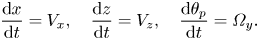 \begin{equation} \dfrac{\textrm{d}x}{\textrm{d}t}=V_x,\quad \dfrac{\textrm{d}z}{\textrm{d}t}=V_z, \quad \dfrac{\textrm{d}\theta_p}{\textrm{d}t}=\varOmega_y. \end{equation}
In the case of a self-diffusiophoretic micromotor near a wall (Mozaffari et al. Reference Mozaffari, Sharifi-Mood, Koplik and Maldarelli2016), the near-wall adjustments in the concentration distribution provide a cushioning effect against the steric collision between the swimmer and the wall. Conversely, in the present situation, the swimmer often approaches very close to the wall, leading to an inevitable crashing against the wall, and no further information about its motion can be retrieved beyond this point. Such a contrast arises due to different physical conditions of the concentration and temperature fields at the plane wall in the respective cases. In the case of a comparable self-diffusiophoretic swimmer, the physical circumstance of the impermeability of solutes at the wall demands a zero-flux boundary condition. Here, on the other hand, the wall is maintained isothermal by using a constant temperature bath therefore allowing a finite normal temperature gradient at the wall. The dimensionless heat flux absorbed by the cold isothermal wall from the heated fluid takes the form
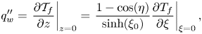 \begin{equation} q''_w= \left.\frac{\partial \mathcal{T}_{f}}{\partial z}\right|_{z=0}= \left.\frac{1-\cos(\eta)}{\sinh(\xi_0)}\frac{\partial T_f}{\partial \xi} \right|_{\xi=0}, \end{equation}
which upon using (2.7) yields
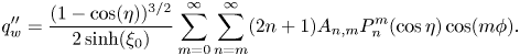 \begin{equation} q''_w=\frac{(1-\cos(\eta))^{3/2}}{2\sinh(\xi_0)} \sum_{m=0}^{\infty}\sum_{n=m}^{\infty} (2 n+1) A_{n,m} P_n^{m}(\cos\eta)\cos(m\phi). \end{equation}
This allows for corresponding adjustments in the temperature distribution keeping the whole wall-adjacent region cool, conforming to the boundary condition of a cold wall. As a consequence, the accumulation of heat in the gap between the particle and wall is nullified. Such a physical scenario is in stark contrast to the comparable self-diffusiophoretic problem where solute molecules are forced to accumulate in the gap, leading to a fluid flow favourable for the near-wall cushioning characteristics. Another wall boundary condition analysed in relation to self-diffusiophoreis is the one having chemiosmotic slip (Uspal et al. Reference Uspal, Popescu, Dietrich and Tasinkevych2016). An analogous system for a self-thermophoretic swimmer should contain a varying temperature boundary condition at the wall, allowing for a thermo-osmotic slip (Lou et al. Reference Lou, Yu, Liu, Chen and Yang2018). This has been left as an intriguing extension of the present work.
The problem of steric collision has been circumvented by employing an electrostatic-type, short-ranged repulsive force at the plane wall (Spagnolie & Lauga Reference Spagnolie and Lauga2012):
 \begin{equation} \boldsymbol{F}_{rep}= \dfrac{\alpha_1 \exp{(-\alpha_2 \delta)}}{1-\exp{(-\alpha_2 \delta)}} \hat{\boldsymbol{e}}_{\boldsymbol{z}} . \end{equation}
The parameters  $\alpha _1,\alpha _2$ have typical values 200, 100, respectively, so that the swimmer does not approach closer than
  $\approx$0.01 times the swimmer radius. Such a scenario was previously encountered by others in relation to ‘squirmers’ (Spagnolie & Lauga Reference Spagnolie and Lauga2012; Li & Ardekani Reference Li and Ardekani2014; Poddar, Bandopadhyay & Chakraborty Reference Poddar, Bandopadhyay and Chakraborty2020), as well as self-diffusiophoretic microswimmers (Ibrahim & Liverpool Reference Ibrahim and Liverpool2016), and different forms of repulsive potentials were employed. It is noteworthy that the squirmer models only deal with the hydrodynamics of the microswimmer, and the wall-induced distortion of the scalar field (e.g. temperature or solute) is not captured. Hence, the wall-bounded motion of an auto-thermophoretic microswimmer cannot be predicted by either of the self-diffusiophoretic or the squirmer models.
An alternative solution approach based on the singular perturbation theory can be adopted to alleviate the divergence or extreme slow convergence of the flow field in the near-contact regime, as described by others (O'neill & Stewartson Reference O'neill and Stewartson1967; Yariv & Brenner Reference Yariv and Brenner2003). However, it was shown by O'neill & Stewartson (Reference O'neill and Stewartson1967) that the presently adopted exact approach using infinite series gives accurate results even for sphere-wall distances as small as  $\delta =2 \times 10^{-4}$, which is far lower than the approximate minimum distances considered in this study, i.e.
  $\delta \approx 0.01$ (also known as cutoff distance). In the present case, the infinite series have been truncated to
  $n_{max}=70$ terms for the lowest distance considered. This has been chosen to ensure that the various series coefficients in the temperature distribution ((2.7)) as well as the complementary flow fields (details in Dean & O'Neill Reference Dean and O'Neill1963, O'Neill Reference O'Neill1964 and Pasol et al. Reference Pasol, Chaoui, Yahiaoui and Feuillebois2005) converge with an error of
  ${\le } 10^{-6}$ between the series coefficients corresponding to
  $n_{max}$ and
  $n_{max}+1$.
Some of the limiting circumstances in the micromotor trajectory have to be treated cautiously. As  $\varphi _{cap} \to 180^\circ$, the temperature asymmetry about the director
  $\boldsymbol {{d}}$ vanishes completely, and motion of the particle is similar to a uniformly heated particle near a wall. In this condition, asymmetric distribution of the driving influences provides an attractive force along the ‘
 $-z$’ direction, leading to a ‘direct impact’ onto the wall. Virtually, a similar scenario of swimmer trajectory arises if the micromotor is launched with director pointing along
  $`-z$’ (i.e.
  $\theta _{p,0}=180^\circ$, where
  $\theta _{p,0}$ is the initial launching orientation of the micromotor), irrespective of the coverage angle,
  $\varphi _{cap}$. It is to be noted that a fully covered particle should not, ideally, have a director because the concept of director exists only for an asymmetric particle. However, for consistency in mathematical analysis, that condition has been treated here as a limit when the coating coverage angle becomes increasingly higher, which is mathematically equivalent to
  $\varphi _{cap} \to 180^{\circ }$. The condition
  $\theta _{p,0}=0^\circ$ is relatively involved. In that case, consistent with the common intuition, the swimmer escapes along an upward straight line as long as the cap coverage angle (
 $\varphi _{cap}$) is below a critical value. Beyond this
  $\varphi _{cap}$, the downward attraction effect due to the wall (discussed later) becomes prominent, and a downward direct impact occurs. The ‘direct impact’ and ‘upward escape’ swimming states have been denoted by black and blue triangles, respectively, in the phase diagrams to follow.
3.5.1. Swimming-state transitions due to thermal conductivity contrast
In the following discussion, different swimming trajectories are categorized and described focusing on the results where a characteristic shift of the trajectories takes place due to the variations in the particle-to-fluid thermal conductivity ratio.
3.5.2. Case-I: From sliding to escape with small heated cap
In figure 11(a), the swimming trajectories of the micromotor have been illustrated with the help of a phase diagram on the  $\mathcal {K}-\theta _{p,0}$ plane for a cap coverage angle of
  $\varphi _{cap}=25^\circ$ and initial launching height of
  $h_0=2$. For low values of
  $\mathcal {K}$, until a launching orientation
  $\theta _{p,0} \lesssim 77.5^\circ$ (the increment of
  $\theta _{p,0}$ considered here is
  $2.5^\circ$), the micromotor only escapes away from the wall, never to return. However, when the swimmer is launched from an orientation leaning more towards the wall, the swimmer slides along the wall, keeping a small gap from it and maintaining a fixed angular orientation. The scenario changes as the thermal conductivity ratio
  $\mathcal {K}$ increases beyond a critical value of
  $\mathcal {K}_{cr} \approx 1.30$. (The critical values of
  $\mathcal {K}$ are found with a fine resolution until an accuracy of first two significant digits is obtained.) With the initial orientations more towards the wall, the
  $\mathcal {K}_{cr}$ value becomes higher, and eventually for
  $\theta _{p,0} \gtrsim 82.5 ^\circ$, the sliding to escape transition onsets at
  $\mathcal {K}_{cr} \approx 7.15$.
Figure 11. Case-I: (a) phase map of the microswimmer trajectories on the  $\mathcal {K}-\theta _{p,0}$ plane. (b) Comparison of swimming trajectories for different thermal conductivity contrast with
  $\theta _{p,0}=90^{\circ }$. In panel (i),
  $\mathcal {K}=10$, and in panel (ii),
  $\mathcal {K}=5$. In panel (i), the microswimmer escapes from the wall and attains a fixed orientation
  $\theta _p= 48.7 ^{\circ }$. In panel (ii), it slides along the wall with a fixed velocity of
  $V_{slide}= 0.018$ with a fixed orientation
  $\theta _{p,end}= 33.23 ^{\circ }$. For both panels (a) and (b), we have chosen
  $\varphi _{cap}=25^{\circ }$ and
  $h_ 0=2$. (c) Variation of sliding velocity
  $(V_{slide})$ and final orientation angle
  $(\theta _{p,{end}})$ with
  $\mathcal {K}<\mathcal {K}_{cr}$ as per panel (b). Panels (d,e) correspond to the variations in
  $\theta _{p}$ and
  $\theta _{v}$ for the trajectories in panels (b)(i) and (b)(ii), respectively. Hereafter, the yellow arrows on micromotors indicate the instantaneous director orientations in that trajectory. Black arrows in panel (b) indicate the direction of impending motion, while the corresponding director direction
  $(\theta _p)$ and trajectory direction
  $(\theta _v)$ are shown in panels (d) and (e).
Figure 11(b) demonstrates two typical trajectories of a micromotor launched from  $\theta _{p,0}=90^\circ$ with
  $\mathcal {K}$ values below or above the critical one. In both the cases, the micromotor shows an impending motion with
  $\varOmega _y<0$ and
  $V_z<0$. Now, similar to our previous discussions in § 3.1, a micromotor with
  $\mathcal {K}=5$ experiences stronger surface temperature gradient in comparison with its
  $\mathcal {K}=10$ counterpart. This condition promotes a subsequent raise in the horizontal component of micromotor velocity
  $(+V_x)$ as well as causing a faster migration in the vertically downward direction
  $(-V_z)$. Under the competitive driving forces for rotation (refer to § 3.3), once a critical condition is reached, the micromotor experiences a net-zero rotation rate,
  $\varOmega _y=0$. Here, the hydrodynamic resistance to the downward approach is not sufficient to prevent a steric collision, and the repulsive force
  $(\boldsymbol {F}_{rep})$ plays its role by contributing to the upward resistive force, leading to a net-zero vertical velocity, i.e.
  $V_z=0$. In contrast to this, with
  $\mathcal {K}=10$, a micromotor with a lesser amount of counterclockwise rotation also experiences a reduced hydrodynamic resistance. Still, it continues to rotate while remaining in the wall-adjacent region. Eventually, the angular orientation reaches a point where the particle gains an upward velocity component
  $(V_z>0)$, and it is ultimately reflected from the wall. As it moves upward, the rotation becomes diminishingly small, thereby letting the particle proceed with a fixed orientation of
  $48.7^\circ$.
The increasing particle conductivity not only causes a characteristic shift of the trajectories but also results in modulations in the sliding velocity and the fixed tilt angle with which the swimmer traverses (see figure 11c). As the particle-to-fluid thermal conductivity ratio increases towards the critical value, the sliding velocity diminishes, and the director tilts more towards the wall.
The figures 11(d) and 11(e) depict the variations of the angle of the propulsion direction,  $\theta _v$, and the director orientation,
  $\theta _p$, as the particle moves in the trajectories in figure 11(b)(i) and figure 11(b)(ii), respectively. The deviations of the near-wall propulsion directions
  $(\theta _v)$ from the unbounded case (showing propulsion along
  $\theta _p$) become clear from these figures.
3.5.3. Case-II: From stopping to escape with small heated cap
Here, we present the case when the micromotor has a small heated cap, and a transition from stationary to escaping trajectories takes place for a critical value of the thermal conductivity ratio  $\mathcal {K}_{cr}$. This critical condition can be realized for either of the following conditions: (i) the fluid is more conductive than the particle (demonstrated in figure 12a) or (ii) the particle is more conductive than the fluid (figure 12b). Comparing figures 12(a) and 12(b), we find that the critical thermal conductivity contrast shifts from
  $\mathcal {K}_{cr}\approx 0.17$ to 3.7, as the heated area increases from
  $\varphi _{cap}=40^\circ$ to
  $50^\circ$. Figure 12(c)(ii) depicts that, before the critical condition in the phase diagram is reached
  $(\mathcal {K}<0.17)$, the micromotor comes very close to the wall while rotating in the counterclockwise direction under strong thermophoretic propulsive torque. Soon it reaches a condition where the director
  $(\boldsymbol { d})$ points vertically upward, i.e.
  $\theta _{p,end}=0$. Such an equilibrium orientation lacks any driving force for axial migration (i.e.
  $V_x=0$) as well as rotation (i.e.
  $\varOmega _y=0$). At the same time, the downward phoretic thrust force is balanced by the tremendous hydrodynamic resistive force and the repulsive potential of the wall
  $\boldsymbol {F}_\text {rep}$. Thus, the motion of the swimmer is completely arrested, and it reaches a ‘stationary’ state. However, when the
  $\mathcal {K}$ value increases beyond
  $\mathcal {K}_{cr}$ (refer to figure 12c(i)), the counterclockwise rotation is weaker, and it migrates downward at a slower pace. As a result, well before the orientation reaches the
  $\theta _p=0$ state, the micromotor attains the critical position for the reversal of
  $-V_z$ to
  $+V_z$, a phenomenon causing a reflecting trajectory similar to figure 11(b)(i).
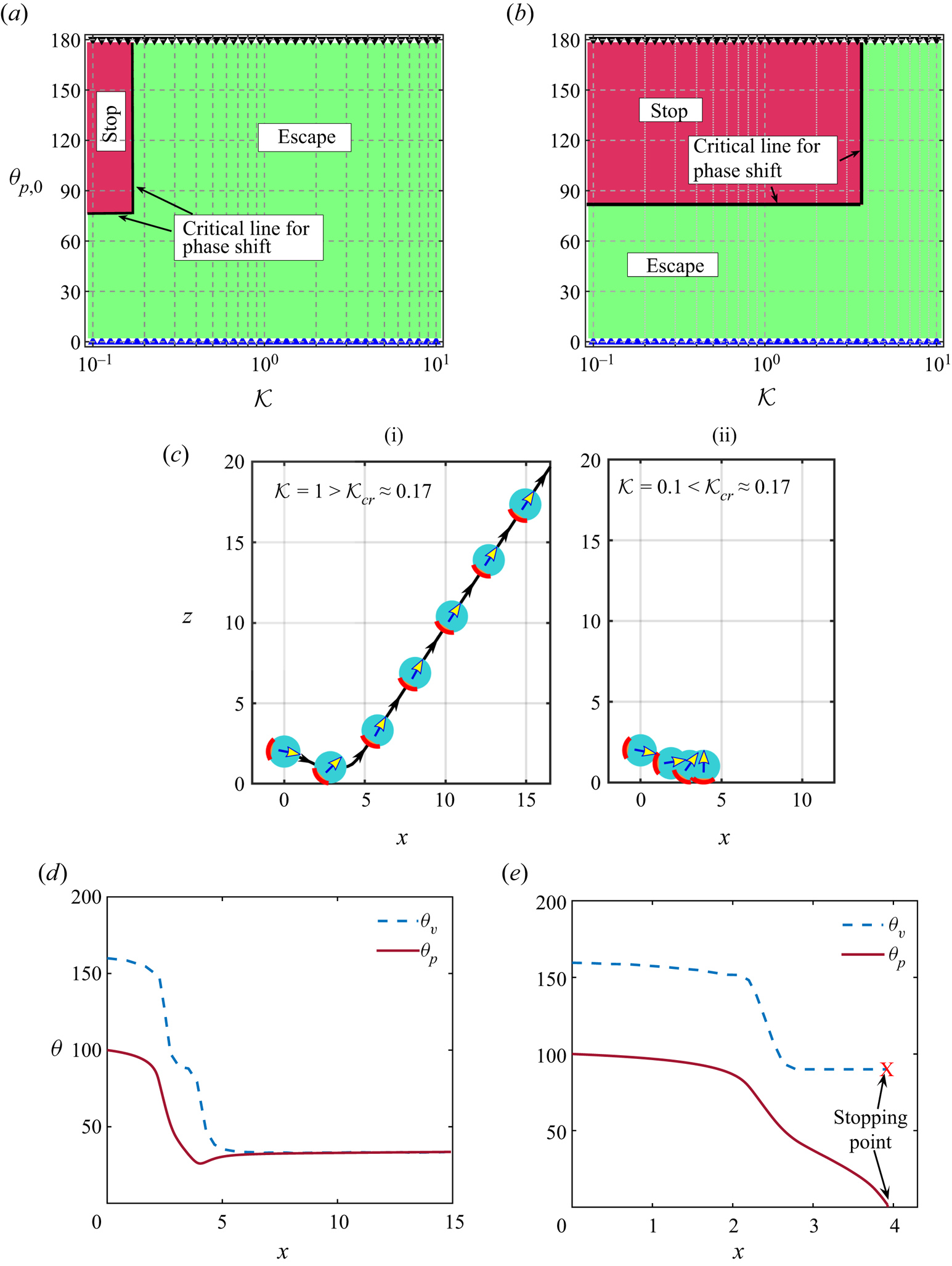
Figure 12. Case-II: (a,b) phase map of the microswimmer trajectories on the  $\mathcal {K}-\theta _{p,0}$ plane for coverage angles
  $\varphi _{cap}=40 ^{\circ }$ and
  $50^{\circ }$, respectively. In both panels,
  $h_0=2$. (c) Comparison of swimming trajectories for different thermal conductivity contrast with
  $\theta _{p,0}=100 ^{\circ }$ and
  $\varphi _{cap}=40 ^{\circ }$. In panel (i),
  $\mathcal {K}=1$, and in panel (ii),
  $\mathcal {K}=0.1$. In panel (i) the microswimmer escapes from the wall and attains a fixed orientation
  $\theta _p= 36.5^{\circ }$. In panel (ii), it becomes stationary at position
 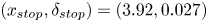 $(x_{stop},\delta _{stop})=(3.92,0.027)$ and a vertical fixed orientation, i.e.
  $\theta _p = 0 ^{\circ }$. In panels (d) and (e), we have shown the variations of
  $\theta _{p}$ and
  $\theta _{v}$ with
  $x$ for the trajectories in panels (c)(i) and (ii), respectively.
For a better insight of the trajectories of figure 12(c)(i) and (ii), we have plotted the variations of the corresponding  $\theta _p$ and
  $\theta _v$ with
  $x$ in figures 12(d) and 12(e), respectively, for those trajectories. Since the particle comes to a standstill in the trajectory of figure 12(c)(ii), the angle
  $\theta _v$ cannot be defined as the swimmer stops. This point has also been highlighted in figures 12(e).
3.5.4. Case-III: From stopping to escape with a large heated cap
Here, the cap coverage is high 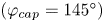 $(\varphi _{cap}=145^\circ )$, but the nature of transition is almost similar to Case-II presented above. The only distinguishing factor in the transition is the height above the wall
  $(\delta _{cr})$ where the sign flip of
  $V_z$ takes place for
  $\mathcal {K}>\mathcal {K}_{cr}$. Similar to Case-I,
  $\mathcal {K}_{cr}$ is a function of the initial orientation
  $(\theta _{p,0})$. Figure 13(a) shows that, in the domain
  $0<\theta _{p,0}<12.5^\circ$, we have
  $\mathcal {K}_{cr} \approx 0.65$, while for
 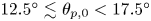 $12.5^\circ \lesssim \theta _{p,0}<17.5^\circ$, we have
  $\mathcal {K}_{cr} \approx 1$. As illustrated in figure 13(b)(i), the micromotor never comes too close to the wall, and the critical height is just below the initial launching height
  $(h_0)$. This provides a sense of repulsive action from the wall at a much greater vertical distance than that in Case-II. It is to be noted that we have not plotted variations of angles
  $\theta _p$ and
  $\theta _v$ in figure 13 because those hardly provide any new information, having already shown the variations of all characteristically different trajectories (escape, slide, stop) for the previous two cases.
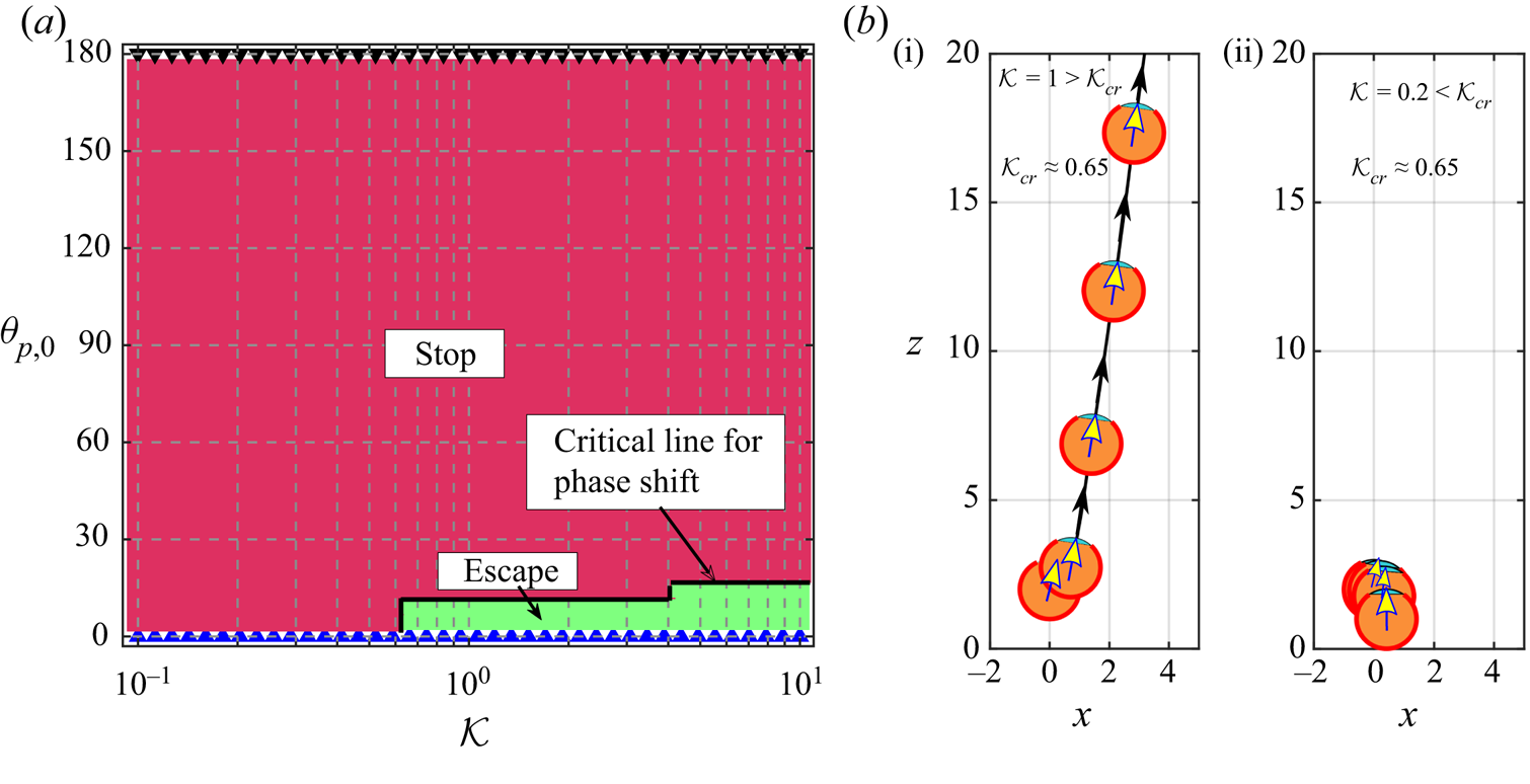
Figure 13. Case-III: (a) phase map of the microswimmer trajectories on the  $\mathcal {K}-\theta _{p,0}$ plane for coverage angle
  $\varphi _{cap}=145^{\circ }$. (b) Comparison of swimming trajectories for different thermal conductivity contrast with
  $\theta _{p,0}=10 ^{\circ },\varphi _{cap}=145^{\circ }$ and
  $h_0=2$. In panel (i),
  $\mathcal {K}=1$, and in panel (ii),
  $\mathcal {K}=0.1$. In panel (i), the microswimmer escapes from the wall and attains a fixed orientation
  $\theta _p= 7.8 ^{\circ }$. In panel (ii), it becomes stationary at position
  $(x_{stop},\delta _{stop})=(0.42,0.015)$ and a vertical fixed orientation, i.e.
  $\theta _{p,stop} = 0 ^{\circ }$.
3.5.5. Influence of initial height, cap coverage and initial orientation
The final swimming feature of the micromotor has been summarized in figure 14(a–c) for all the possible ranges of the heated cap angle  $\varphi _{cap}$ and the initial launching angle
  $\theta _{p,0}$. These figures help elucidate some key differences in the trajectory characteristics with those presented previously in connection with the self-diffusiophoresis phenomenon near a solute-impenetrable plane wall (Uspal et al. Reference Uspal, Popescu, Dietrich and Tasinkevych2015a; Ibrahim & Liverpool Reference Ibrahim and Liverpool2016; Mozaffari et al. Reference Mozaffari, Sharifi-Mood, Koplik and Maldarelli2016). In order to readily compare with such a widely studied problem, the geometry of the swimmer-wall system and the swimmer orientation have been defined in an exactly similar manner to those of Mozaffari et al. (Reference Mozaffari, Sharifi-Mood, Koplik and Maldarelli2016). Firstly, the thermophoretic force is of a strikingly distinct nature in imparting a downward motion to the micromotor even when the director initially faces away from the wall (e.g. in figure 14a). Secondly, in the corresponding problems addressed, it was found that the micromotor does not achieve a velocity of
  $V_z<0$ for any extent of the active area if
  $\theta _{p,0}<90^\circ$. In sharp contrast to these observations, in the present scenario, we observe that the micromotor can have
  $V_z<0$ even when
  $\theta _{p,0}<90^\circ$. An example of this outcome is provided in figure 17 in the Appendix for a typical heated cap coverage of
  $\varphi _{cap}=90^\circ$ and equal conductivities of the two media
  $(\mathcal {K}=1)$.Further, the phase maps in figure 14(a) demonstrate that, when the micromotor has a large heated cap, the zone of stopping points on the maps penetrates the region of
  $\theta _{p,0}<90^\circ$, and even a fully vertical orientation with
  $\theta _{p,0}=0^\circ$ can result in the case of complete stationary trajectories.
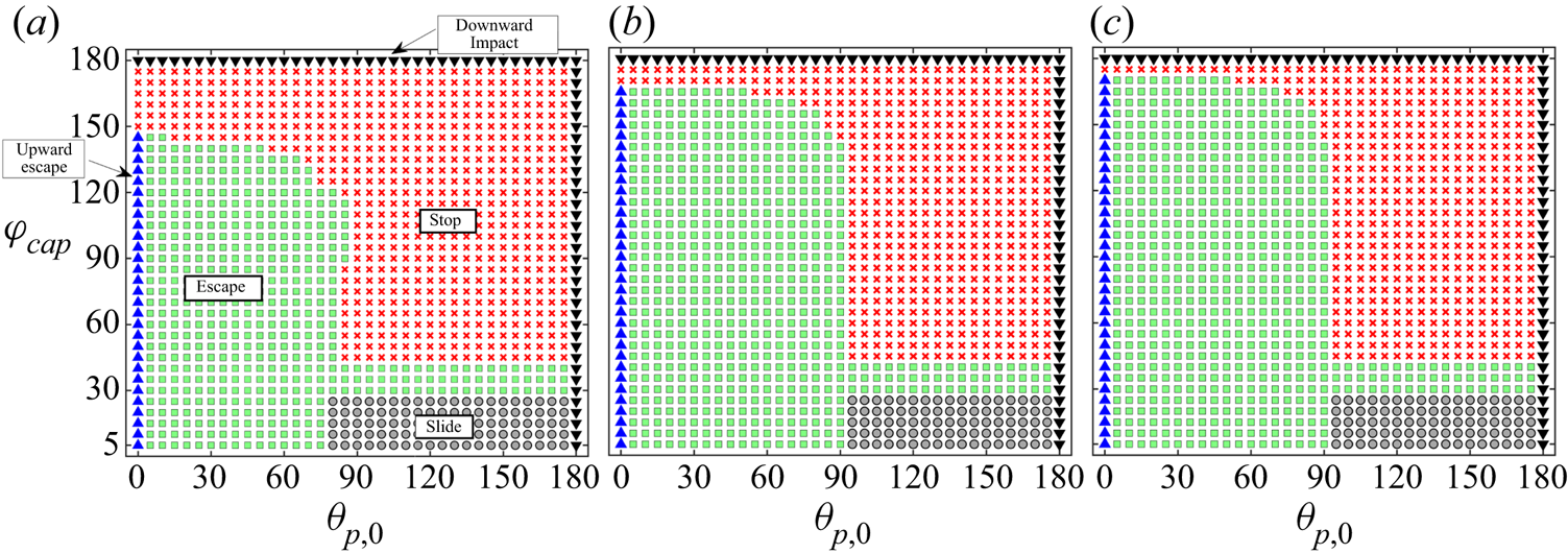
Figure 14. Phase maps categorizing the swimming behaviours of the auto-thermophoretic microswimmer for different values of the coverage angle of the metal cap  $(\varphi _{cap})$ and initial launching angle
  $(\theta _p)$. (a), (b) and (c) correspond to different initial heights as shown. The thermal conductivity ratio has been chosen as
  $\mathcal {K}=1$. Here the phase maps have been constructed on a grid of
  $5^\circ$ intervals on both the coordinates.
  $(a)\, \delta_{0} = 1, (b)\, \delta_{0} = 4,\ (c) \delta_{0} = 6$
As the capped area becomes more extensive, the distortion of the temperature field becomes intrinsically different, which can be visualized by comparing the temperature profiles in figure 15(a,b). This is also reflected in the appearance of two distinct maxima points on the  $\mathcal {T}_S \ \text {vs.} \ \theta$ curves for high
  $\varphi _{cap}$ instead of just one for low cap angle (please refer to figure 15c). Consequently, the pattern of surface slip flow is modified as portrayed schematically in figure 15(a,b). In the former case, the surface slip flow takes place from the colder region (point
  $\mathcal {T}_{min}$ in figure 15a) to the hotter region (point
  $\mathcal {T}_{max}$ in figure 15a), and the particle gains an upward velocity component
  $(V_z>0)$. In contrast to this, for
  $\varphi _{cap}=160^\circ$, the continuity of flow demands a pair of new circulating rolls due to a reorganization of the surface temperature distribution. As a cumulative effect, the downward surface traction surpasses the upward one, and, subsequently, the motion of the micromotor becomes downward (
 $V_z<0$). An involved relationship of
  $V_z$ on both
  $\varphi _{cap}$ and
  $\theta _{p}$ has been presented in figure 15(d). While this only provides an insight into the impending downward or upward motion during launching, a sliding to escape or escape to stopping transition of swimming states takes place due to qualitatively similar reasons of alterations in particle rotation
  $(\varOmega _y)$ and vertical motion
  $(V_z)$ at a critical transition, as discussed in Case-I of § 3.5.1.
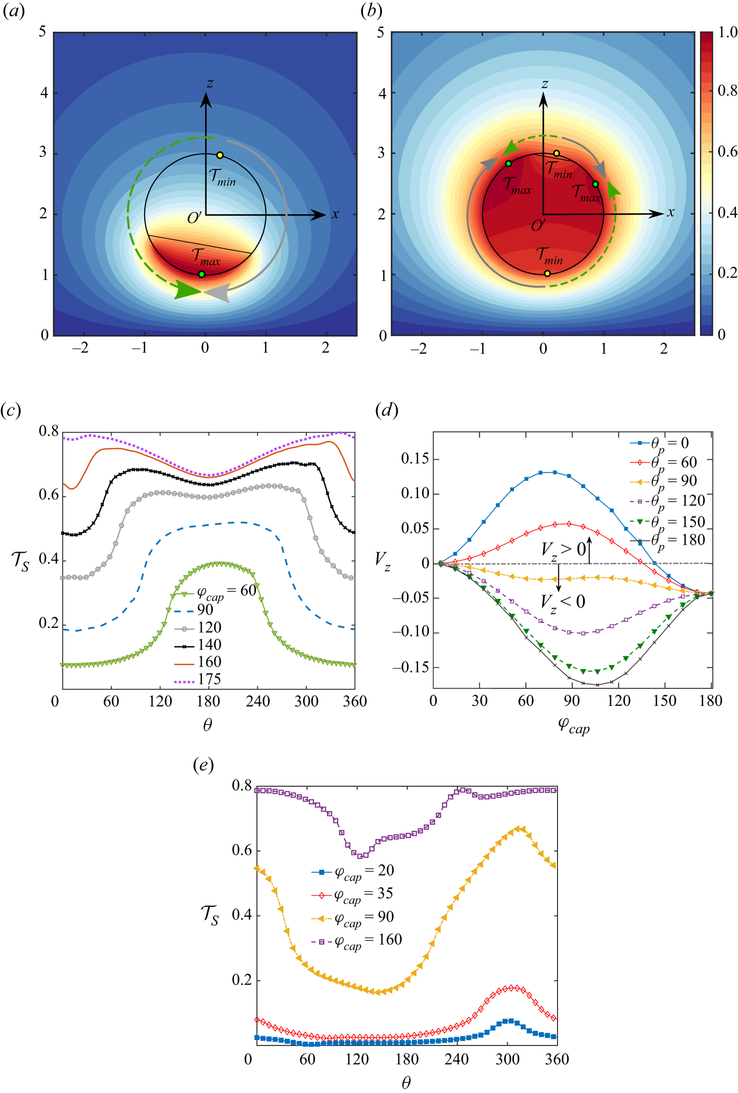
Figure 15. Panels (a,b) show the direction of surface flow for low and high coverage angles  $\varphi _{cap}=60^\circ$ and
  $160^\circ$, respectively. Here, the background colour denotes the scaled temperature field. (c) Variation of surface temperature along the surface of the micromotor for different coverage angles
  $(\varphi _{cap})$. Here,
  $\theta _{p} =10 ^ \circ$ has been chosen for (a–c). (d) Variation of the vertical component of the micromotor velocity
  $(V_z)$ with
  $\varphi _{cap}$ for different
  $\theta _{p}$. (e) Variation of surface temperature along the surface of the micromotor for different coverage angles
  $(\varphi _{cap})$ with
  $\theta _{p}=120^\circ$. Other parameters are chosen as
  $\delta =1$ and
  $\mathcal {K} =1$.
The mechanism by which changing cap angle  $(\varphi _{cap})$ influences the swimmer surface flow is more intricate than the corresponding implication due to thermal conductivity contrast
  $(\mathcal {K})$. We have earlier noted that modulations in
  $\mathcal {K}$ hold the capacity of changing only the relative magnitudes of the peak surface temperatures
 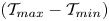 $(\mathcal {T}_{max}-\mathcal {T}_{min} )$, but not the peak locations on the swimmer surface (refer to figure 3). Conversely, the cap angle
  $(\varphi _{cap})$ variation has the potential of shifting the locations of the peak temperatures. Also, it can create or destroy new peak points (see figure 15e for example), thereby regulating the surface flow to a great extent.
Secondly, during the swimming states where the micromotor ends up being motionless, we observe that the director is pointed vertically upward (i.e.  $\theta _{p,end} = 0^\circ$) in the final state (refer to figures 12c(ii) and 13b(ii)). Contrarily, in the previously reported studies (Mozaffari et al. Reference Mozaffari, Sharifi-Mood, Koplik and Maldarelli2016), the final orientation of the stationary states was found to be
 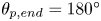 $\theta _{p,end} = 180^\circ$. Also, in the present scenario, the swimmer becomes stationary only after sliding along the wall until it reaches the
  $\theta _p=0^\circ$ condition, while remaining at a close distance from the wall (
 $\delta _{stop} \lesssim 0.1$). However, in the self-diffusiophoresis problems, the micromotor reaches ‘stationary’ states with the final separation height being as high as
  ${\sim}5$ times the particle radius. The difference between the two problem categories also stems from inherently distinguished wall-induced modulations in the peak temperature or solute concentration on the surface of the autophoretic particles considered in the respective cases. Figure 16(a,b) suggest that the minimum temperature location is shifted towards the wall and attains almost a
  $\theta \approx 180^\circ$ position for both the high coverage angles. Moreover, in stark contrast to the study of Mozaffari et al. (Reference Mozaffari, Sharifi-Mood, Koplik and Maldarelli2016), the maximum location shifts towards the north pole with an increase in the coverage angle from
  $\varphi _{cap}=120^\circ$ to
  $150^\circ$. Following the directions of arrows and their altered lengths in figure 16(b) to (a), we find that the contribution of counterclockwise surface traction intensifies. This further causes a net negative rotation leading to
  $\theta _{p,end}=0^\circ$, and the same can be verified from figure 18(b) in the Appendix. Another difference with their work arises from the decreasing values of
  $V_x$, as the swimmer approaches the wall (see figure 18a). Subsequently, the micromotor traverses little distance before coming to rest.
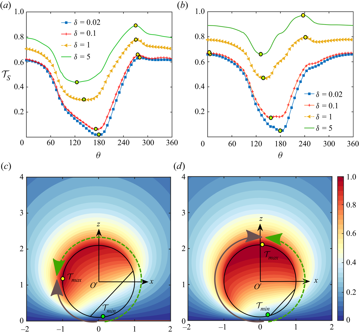
Figure 16. Swimmer surface temperature variation  $(\mathcal {T}_S)$ for different distances from the wall
  $(\delta )$. Panels (a) and (b) correspond to coverage angles of
  $\varphi _{cap}=120^\circ$ and
  $150^\circ$, respectively. (c,d) The solid-black and green-dashed arrows indicate the direction of surface flow. We have chosen
  $\varphi _{cap}=120^\circ$ and
  $150^\circ$, respectively, in the two panels. The background colours denote the scaled temperature field. The other parameters are
  $\mathcal {K}=1$,
  $\delta =0.1$ and
  $\theta _p=135^\circ$. The green and yellow bubbles denote the minimum and maximum temperature locations on the plots, respectively.
When the micromotor is launched from a sufficient height above the planar wall  $(h_0 \sim 10)$, the wall-induced temperature distortions can hardly influence the particle velocity. Accordingly, the micromotor feels a weak attractive force from the wall. Along similar lines, a comparison of the phase maps in figure 14(a–c) reveals that the zone of stopping trajectories in the common region of
  $\theta _p<90^\circ$ and high
  $\varphi _{cap}$ shrinks as the initial height gets increased.
4. Conclusions and remarks
We have explored the capability of navigating a thermally asymmetric micromotor by a nearby isothermal plane wall. The wall-induced temperature distortion in and around the micromotor results is several distinctive characteristics of motion ranging from sliding along the wall, reaching a stationary configuration to getting repelled by the wall at a fixed orientation. Moreover, there exists fixed points for vertical translation at specific swimmer orientations relative to the wall. The present study reveals a unique non-monotonic dependence of the associated critical gap thickness on the extent of metallic coating on the particle surface. However, the thermal conductivity ratio has been found to be incapable of changing the above fixed point characteristics.
For high thermal conductivity contrast between the particle and the fluid, an increasingly significant portion of the particle senses the effect of localized heating due to laser irradiation. This effect, in turn, weakens the temperature gradient and the subsequent phoretic thrust experienced by the micromotor. Our analysis reveals that for a fixed extent of metallic coating and the initial orientation of the micromotor, its final trajectory can be characteristically altered only by changing the particle-to-fluid thermal conductivity contrast. The critical thermal conductivity contrasts responsible for a shift either from sliding to escape or from stopping to escape states have also been reported. It has been found that these critical conditions exist for both the situations of a particle becoming more conductive than the fluid or vice versa. Moreover, the critical thermal conductivity contrast depends on the initial tilt of the micromotor, as demonstrated in figures 11–13.
When a large extent of micromotor surface is coated with the metallic cap, the wall-bound attraction is so strong that migration towards the wall happens, despite the director initially pointing away from the wall. This observation is highly non-intuitive on the backdrop of the previous studies related to self-diffusiophoresis near a wall. Moreover, the zone of sliding states in the phase diagram has shifted from a 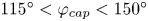 $115^\circ < \varphi _{cap}<150^\circ$ (Mozaffari et al. Reference Mozaffari, Sharifi-Mood, Koplik and Maldarelli2016) condition to
 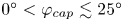 $0^\circ < \varphi _{cap} \lesssim 25^\circ$. Also, a window of intermediate
  $\varphi _{cap}$ values appears:
 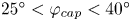 $25^\circ <\varphi _{cap}<40^\circ$, which is sandwiched between the sliding and stopping states. When the micromotor ends up being stationary, it reaches a configuration with the heated surface facing towards the wall.
Since the adiabatic wall effects on the locomotion of a self-thermophoretic micromotor may be perceived by drawing analogies with the reported studies on self-diffusiophoretic transport, and the corresponding effects of an isothermal wall are addressed in this study, the present study may be extended to a generic theoretical platform accommodating arbitrary variations in wall temperature, considering that a generic boundary condition may be represented by a combination of successive isothermal and adiabatic states.
The fundamental know-how of the temperature distribution in and around a self-thermophoretic micromotor and its trajectory characteristics in the vicinity of a plane obstacle with a known thermal condition may be extremely beneficial in designing a novel microscale thermal sensor. While designing an experimental set-up relevant to the present study, qualitative intuitions may be obtained from the passive diffusiophoresis experiments (e.g. Shimokusu et al. Reference Shimokusu, Maybruck, Ault and Shin2019) where the wall has an approximately constant solute concentration boundary condition or from the analysis with a constant chemical potential boundary condition (Warren Reference Warren2020).
The ability to cause critical transitions in the locomotion behaviour based on related thermal and configurational parameters, as explored here, may be exploited to achieve precise control over the navigation of micromotor-based systems for a variety of applications where interaction with a confining boundary is inevitable. Further tuning of these interactions with the aid of thermal noise, topographical alterations (Simmchen et al. Reference Simmchen, Katuri, Uspal, Popescu, Tasinkevych and Sánchez2016) and patterning of the thermal boundary conditions at the wall may be harnessed in the future to achieve desired transitions in swimming states over reduced length scales.
Acknowledgements
A.P. acknowledges Shashank, a summer intern at I.I.T. Kharagpur, for re-doing some of the analytical calculations.
Funding
S.C. acknowledges Department of Science and Technology, Government of India, for Sir J. C. Bose National Fellowship.
Conflicts of interest
The authors declare no conflicts of interest.
Appendix. Detailed variation of velocity components
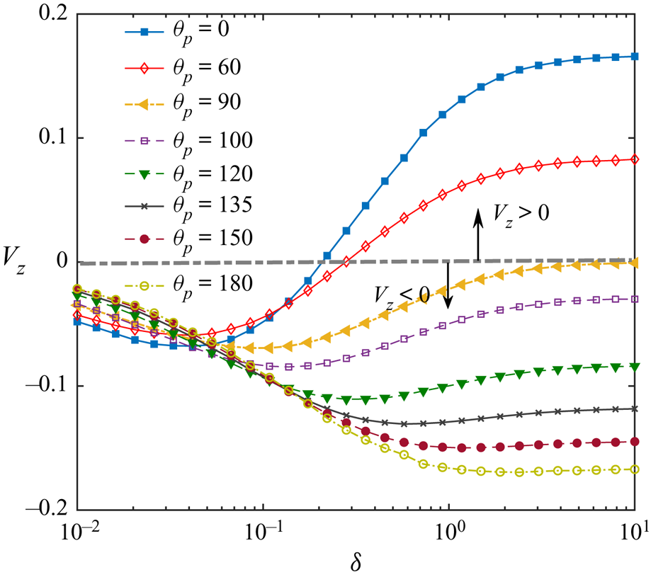
Figure 17. Vertical microswimmer velocity vs. its distance from the wall for different orientation angle  $(\theta _p)$. Here the fixed parameters are
  $\varphi _{cap}=90^\circ$ and
  $\mathcal {K}=1$.
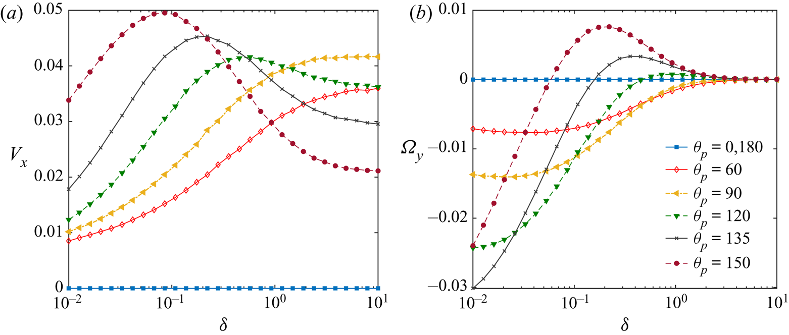
Figure 18. Variation of wall-parallel translational and rotational velocities of the microswimmer with distance from the wall  $(\delta )$ for different orientation angles
  $(\theta _{p})$. Other parameters are chosen as
  $\varphi _{cap} =150 ^{\circ }$ and
  $\mathcal {K} =1$.


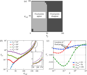


 Open access