


1 Introduction
Cluster algebras were introduced by Fomin and Zelevinsky [Reference Fomin and ZelevinskyFZ02] as a class of commutative algebras equipped with a combinatorial structure relating different subsets of the algebra called clusters. Since then, there has been a great interest in cluster algebras and their relation to other subjects, including Teichmüller theory, polyhedral surfaces, representation theory of quivers and aspects of noncommutative algebraic geometry such as Calabi–Yau algebras, Calabi–Yau categories and stability conditions. A survey with many references can be found in [Reference KellerKel08]; we also refer to the cluster-algebra portal [Reference FominFom] for further surveys and information on cluster algebras.
Relevant for this work is a particular class of cluster algebras associated to oriented marked surfaces equipped with an ideal triangulation, introduced in [Reference Gekhtman, Shapiro and VainshteinGSV05, Reference Fock and GoncharovFG06b, Reference Fock and GoncharovFG09] and further studied in [Reference Fomin, Shapiro and ThurstonFST08, Reference Fomin and ThurstonFT18]. These cluster algebras can be described in two different ways. The first perspective is geometric and provides a description in terms of the decorated Teichmüller spaces of the surfaces. The cluster variables arise as lambda lengths, which form the coordinates of the Teichmüller space. These lambda lengths satisfy an analogue of the classical Ptolemy relations, which gives rise to the cluster exchange relations. The second perspective makes direct use of the combinatorics of the ideal triangulation. The mutation matrix used to define the cluster algebra arises as the signed adjacency matrix of the ideal triangulation, which counts the number of incidences of the ideal triangles. The resulting algebra does not depend on the choice of ideal triangulation but only on the underlying marked surface.
This second perspective in particular shows that cluster algebras of marked surfaces can be considered as cluster algebras associated to quivers, which can be categorified via $2$
-Calabi–Yau (CY) triangulated categories, called cluster categories, and
$2$
-Calabi–Yau (CY) triangulated categories, called cluster categories, and $3$
-CY triangulated categories. To describe the
$3$
-CY triangulated categories. To describe the $3$
-CY categorification of the cluster algebra associated to a quiver Q, one chooses a nondegenerate potential W. The
$3$
-CY categorification of the cluster algebra associated to a quiver Q, one chooses a nondegenerate potential W. The $3$
-CY categorification is then given by the derived category of the Ginzburg algebra
$3$
-CY categorification is then given by the derived category of the Ginzburg algebra $\mathscr {G}(Q,W)$
associated to the quiver with potential
$\mathscr {G}(Q,W)$
associated to the quiver with potential $(Q,W)$
. The
$(Q,W)$
. The $2$
-CY cluster category can be obtained from the derived category of the Ginzburg algebra via the Verdier quotient
$2$
-CY cluster category can be obtained from the derived category of the Ginzburg algebra via the Verdier quotient $\mathcal {D}(\mathscr {G}(Q,W))^{\operatorname {perf}}/\mathcal {D}(\mathscr {G}(Q,W))^{\operatorname {fin}}$
[Reference AmiotAmi09]. There is also a direct link between the Ginzburg algebras and the combinatorics of the cluster algebras; we refer to [Reference KellerKel12] for a survey.
$\mathcal {D}(\mathscr {G}(Q,W))^{\operatorname {perf}}/\mathcal {D}(\mathscr {G}(Q,W))^{\operatorname {fin}}$
[Reference AmiotAmi09]. There is also a direct link between the Ginzburg algebras and the combinatorics of the cluster algebras; we refer to [Reference KellerKel12] for a survey.
To describe the results of this work, we first recall the construction of the quiver $Q_{\mathcal {T}}^{\circ }$
, and a choice of nondegenerate potential
$Q_{\mathcal {T}}^{\circ }$
, and a choice of nondegenerate potential $W_{\mathcal {T}}$
, associated to an ideal triangulation
$W_{\mathcal {T}}$
, associated to an ideal triangulation $\mathcal {T}$
of a marked surface
$\mathcal {T}$
of a marked surface $\mathbf {S}$
[Reference Labardini-FragosoLF09, Reference Geiß, Labardini-Fragoso and SchröerGLFS16]. We assume for simplicity that
$\mathbf {S}$
[Reference Labardini-FragosoLF09, Reference Geiß, Labardini-Fragoso and SchröerGLFS16]. We assume for simplicity that $\mathcal {T}$
has no self-folded triangles. The quiver
$\mathcal {T}$
has no self-folded triangles. The quiver $Q^{\circ }_{\mathcal {T}}$
has as vertices the internal edges of
$Q^{\circ }_{\mathcal {T}}$
has as vertices the internal edges of $\mathcal {T}$
and an arrow
$\mathcal {T}$
and an arrow $a:i\rightarrow j$
for each ideal triangle containing the edges
$a:i\rightarrow j$
for each ideal triangle containing the edges $i,j$
, where the edge j follows the edge i in the clockwise order of the edges of the ideal triangle induced by the orientation of the surface. The nondegenerate potential
$i,j$
, where the edge j follows the edge i in the clockwise order of the edges of the ideal triangle induced by the orientation of the surface. The nondegenerate potential $W_{\mathcal {T}}=W^{\prime }_{\mathcal {T}}+W^{\prime \prime }_{\mathcal {T}}\in kQ^{\circ }_{\mathcal {T}}$
consists of a part
$W_{\mathcal {T}}=W^{\prime }_{\mathcal {T}}+W^{\prime \prime }_{\mathcal {T}}\in kQ^{\circ }_{\mathcal {T}}$
consists of a part $W^{\prime }_{\mathcal {T}}$
which is the sum of the clockwise
$W^{\prime }_{\mathcal {T}}$
which is the sum of the clockwise $3$
-cycles inscribed in the interior ideal triangles of
$3$
-cycles inscribed in the interior ideal triangles of $\mathcal {T}$
and a part
$\mathcal {T}$
and a part $W^{\prime \prime }_{\mathcal {T}}$
which is a sum of anticlockwise cycles, one for each interior marked point of
$W^{\prime \prime }_{\mathcal {T}}$
which is a sum of anticlockwise cycles, one for each interior marked point of $\mathbf {S}$
.
$\mathbf {S}$
.
The $2$
-CY and
$2$
-CY and $3$
-CY categorifications can be described in terms of the combinatorial geometry of
$3$
-CY categorifications can be described in terms of the combinatorial geometry of $\mathcal {T}$
– see [Reference Qiu and ZhouQZ17] and the references therein for the
$\mathcal {T}$
– see [Reference Qiu and ZhouQZ17] and the references therein for the $2$
-CY cluster category and [Reference QiuQiu18, Reference Qiu and ZhouQZ19] for the finite part of the derived category of the Ginzburg algebra
$2$
-CY cluster category and [Reference QiuQiu18, Reference Qiu and ZhouQZ19] for the finite part of the derived category of the Ginzburg algebra $\mathscr {G}\left (Q_{\mathcal {T}}^{\circ },W^{\prime }_{\mathcal {T}}\right )$
. Most relevant for us is Ivan Smith’s realisation of the finite part of the derived category of
$\mathscr {G}\left (Q_{\mathcal {T}}^{\circ },W^{\prime }_{\mathcal {T}}\right )$
. Most relevant for us is Ivan Smith’s realisation of the finite part of the derived category of $\mathscr {G}\left (Q_{\mathcal {T}}^{\circ },W_{\mathcal {T}}^{\prime }\right )$
as a full subcategory of the Fukaya category of a Calabi–Yau
$\mathscr {G}\left (Q_{\mathcal {T}}^{\circ },W_{\mathcal {T}}^{\prime }\right )$
as a full subcategory of the Fukaya category of a Calabi–Yau $3$
-fold
$3$
-fold $Y^{\circ }$
equipped with a Lefschetz fibration
$Y^{\circ }$
equipped with a Lefschetz fibration $\pi :Y^{\circ }\rightarrow \Sigma $
[Reference SmithSmi15]. The surface
$\pi :Y^{\circ }\rightarrow \Sigma $
[Reference SmithSmi15]. The surface $\Sigma $
is obtained from
$\Sigma $
is obtained from $\mathbf {S}$
by removing all interior marked points – that is,
$\mathbf {S}$
by removing all interior marked points – that is, $\Sigma = \mathbf {S}\backslash (M\cap \mathbf {S}^{\circ })$
, where
$\Sigma = \mathbf {S}\backslash (M\cap \mathbf {S}^{\circ })$
, where $\mathbf {S}^{\circ }=\mathbf {S}\backslash \partial \mathbf {S}$
denotes the interior of
$\mathbf {S}^{\circ }=\mathbf {S}\backslash \partial \mathbf {S}$
denotes the interior of $\mathbf {S}$
and M denotes the set of marked points. Inspired by the geometry of
$\mathbf {S}$
and M denotes the set of marked points. Inspired by the geometry of $\pi $
, we give in this paper a description of the entire unbounded derived category of the Ginzburg algebra
$\pi $
, we give in this paper a description of the entire unbounded derived category of the Ginzburg algebra $\mathscr {G}\left (Q_{\mathcal {T}}^{\circ },W_{\mathcal {T}}^{\prime }\right )$
in terms of the global sections of a perverse schober.
$\mathscr {G}\left (Q_{\mathcal {T}}^{\circ },W_{\mathcal {T}}^{\prime }\right )$
in terms of the global sections of a perverse schober.
Before we describe our model for $\mathcal {D}\left (\mathscr {G}\left (Q_{\mathcal {T}}^{\circ },W_{\mathcal {T}}^{\prime }\right )\right )$
, we highlight the relation to a model for the partially wrapped Fukaya categories of graded surfaces or, equivalently, the derived categories of gentle algebras [Reference Haiden, Katzarkov and KontsevichHKK17, Reference Lekili and PolishchukLP20]. Consider an ideal triangulation of a graded marked surface
$\mathcal {D}\left (\mathscr {G}\left (Q_{\mathcal {T}}^{\circ },W_{\mathcal {T}}^{\prime }\right )\right )$
, we highlight the relation to a model for the partially wrapped Fukaya categories of graded surfaces or, equivalently, the derived categories of gentle algebras [Reference Haiden, Katzarkov and KontsevichHKK17, Reference Lekili and PolishchukLP20]. Consider an ideal triangulation of a graded marked surface $\mathbf {S}$
and the dual ribbon graph
$\mathbf {S}$
and the dual ribbon graph $\Gamma $
. The Fukaya category of the surface
$\Gamma $
. The Fukaya category of the surface $\mathbf {S}$
is equivalent to the dg-category of global sections of a constructible cosheaf of dg-categories on the ribbon graph
$\mathbf {S}$
is equivalent to the dg-category of global sections of a constructible cosheaf of dg-categories on the ribbon graph $\Gamma $
[Reference Dyckerhoff and KapranovDK15, Reference Haiden, Katzarkov and KontsevichHKK17]. The cosheaf description of the Fukaya category categorifies the statement that the middle cohomology
$\Gamma $
[Reference Dyckerhoff and KapranovDK15, Reference Haiden, Katzarkov and KontsevichHKK17]. The cosheaf description of the Fukaya category categorifies the statement that the middle cohomology $\operatorname {H}_{\Gamma }(\Sigma ,\mathbb {Z}[1])$
of the surface
$\operatorname {H}_{\Gamma }(\Sigma ,\mathbb {Z}[1])$
of the surface $\Sigma $
with support on
$\Sigma $
with support on $\Gamma $
is equivalent to the abelian group of global sections of a constructible cosheaf
$\Gamma $
is equivalent to the abelian group of global sections of a constructible cosheaf $\underline {\operatorname {H}}_{\Gamma }(\mathbb {Z}[1])$
on
$\underline {\operatorname {H}}_{\Gamma }(\mathbb {Z}[1])$
on $\Gamma $
whose stalk at a point x is the homology
$\Gamma $
whose stalk at a point x is the homology $\operatorname {H}_{\Gamma \cap U}(U,\mathbb {Z}[1])$
of a small neighbourhood
$\operatorname {H}_{\Gamma \cap U}(U,\mathbb {Z}[1])$
of a small neighbourhood $x\in U\subset \Sigma $
with support on
$x\in U\subset \Sigma $
with support on $\Gamma \cap U$
. Our model describes the derived category of the Ginzburg algebra in terms of the global sections of a different constructible cosheaf of dg-categories on
$\Gamma \cap U$
. Our model describes the derived category of the Ginzburg algebra in terms of the global sections of a different constructible cosheaf of dg-categories on $\Gamma $
. Denote by
$\Gamma $
. Denote by $\Gamma ^{\circ }$
the ribbon graph obtained by removing all exterior edges of
$\Gamma ^{\circ }$
the ribbon graph obtained by removing all exterior edges of $\Gamma $
. Decategorified, the idea behind our model is to express the middle cohomology of the
$\Gamma $
. Decategorified, the idea behind our model is to express the middle cohomology of the $3$
-fold
$3$
-fold $Y^{\circ }$
with support on
$Y^{\circ }$
with support on $\pi ^{-1}(\Gamma ^{\circ })$
in terms of the abelian group of global sections with support on
$\pi ^{-1}(\Gamma ^{\circ })$
in terms of the abelian group of global sections with support on $\Gamma ^{\circ }$
of the perverse push-forward
$\Gamma ^{\circ }$
of the perverse push-forward $\pi _{*}(\mathbb {Z}[3])$
to
$\pi _{*}(\mathbb {Z}[3])$
to $\Sigma $
, which in turn is equivalent to the global sections with support on
$\Sigma $
, which in turn is equivalent to the global sections with support on $\Gamma ^{\circ }$
of a constructible cosheaf
$\Gamma ^{\circ }$
of a constructible cosheaf $\underline {\operatorname {H}}_{\Gamma }(\pi _{*}\mathbb {Z}[3])$
on
$\underline {\operatorname {H}}_{\Gamma }(\pi _{*}\mathbb {Z}[3])$
on $\Gamma $
. We will not provide a systematic categorification of the perverse push-forward functor
$\Gamma $
. We will not provide a systematic categorification of the perverse push-forward functor $\pi _{*}$
, but rather provide an explicit description of the categorification of the constructible cosheaf
$\pi _{*}$
, but rather provide an explicit description of the categorification of the constructible cosheaf $\underline {\operatorname {H}}_{\Gamma }(\pi _{*}\mathbb {Z}[3])$
. This will be achieved by constructing a perverse schober on the surface that is classified locally, at every critical value of Smith’s Lefschetz fibration, by the
$\underline {\operatorname {H}}_{\Gamma }(\pi _{*}\mathbb {Z}[3])$
. This will be achieved by constructing a perverse schober on the surface that is classified locally, at every critical value of Smith’s Lefschetz fibration, by the $\operatorname {Ind}$
-complete version of the spherical adjunction
$\operatorname {Ind}$
-complete version of the spherical adjunction
 $$ \begin{align*} \mathcal{W}\left(T^{*}S^{2}\right) \longleftrightarrow \mathcal{D}(k)^{\operatorname{perf}}. \end{align*} $$
The explicit computability of our model then arises from a concrete algebraic description of this adjunction, as well as the resulting categorification of $\underline {\operatorname {H}}_{\Gamma }(\pi _{*}\mathbb {Z}[3]))$
in terms of variants of Waldhausen’s
$\underline {\operatorname {H}}_{\Gamma }(\pi _{*}\mathbb {Z}[3]))$
in terms of variants of Waldhausen’s $\operatorname {S}_{\bullet }$
-construction. A full definition of the notion of a perverse schober on a surface is not yet documented in the literature; we thus introduce a framework for the treatment of perverse schobers on surfaces which are parametrised by ribbon graphs. Our definition of a parametrised perverse schober can be seen as a generalisation of the approach to topological Fukaya categories of surfaces of [Reference Dyckerhoff and KapranovDK18, Reference Dyckerhoff and KapranovDK15], allowing for the treatment of nonconstant coefficients. The main result of this paper is the following:
$\operatorname {S}_{\bullet }$
-construction. A full definition of the notion of a perverse schober on a surface is not yet documented in the literature; we thus introduce a framework for the treatment of perverse schobers on surfaces which are parametrised by ribbon graphs. Our definition of a parametrised perverse schober can be seen as a generalisation of the approach to topological Fukaya categories of surfaces of [Reference Dyckerhoff and KapranovDK18, Reference Dyckerhoff and KapranovDK15], allowing for the treatment of nonconstant coefficients. The main result of this paper is the following:
Theorem 1. Let $\mathcal {T}$
be an ideal triangulation of an oriented marked surface
$\mathcal {T}$
be an ideal triangulation of an oriented marked surface $\mathbf {S}$
and consider the dual ribbon graph
$\mathbf {S}$
and consider the dual ribbon graph $\Gamma $
. There exists a
$\Gamma $
. There exists a $\Gamma $
-parametrised perverse schober
$\Gamma $
-parametrised perverse schober $\mathcal {F}_{\mathcal {T}}$
whose stable
$\mathcal {F}_{\mathcal {T}}$
whose stable $\infty $
-category of global sections with support on
$\infty $
-category of global sections with support on $\Gamma ^{\circ }$
satisfies
$\Gamma ^{\circ }$
satisfies
 $$ \begin{align*} \mathcal{H}_{\Gamma^{\circ}}(\Gamma,\mathcal{F}_{\mathcal{T}})\simeq \mathcal{D}\left(\mathscr{G}\left(Q^{\circ}_{\mathcal{T}},W^{\prime}_{\mathcal{T}}\right)\right). \end{align*} $$
That is, it is equivalent to the unbounded derived $\infty $
-category of the Ginzburg algebra
$\infty $
-category of the Ginzburg algebra $\mathscr {G}\left (Q_{\mathcal {T}}^{\circ },W^{\prime }_{\mathcal {T}}\right )$
.
$\mathscr {G}\left (Q_{\mathcal {T}}^{\circ },W^{\prime }_{\mathcal {T}}\right )$
.
Note that if $\mathcal {T}$
contains no interior marked points, the potential
$\mathcal {T}$
contains no interior marked points, the potential $W^{\prime }_{\mathcal {T}}=W_{\mathcal {T}}$
is nondegenerate. Given an ideal triangulation
$W^{\prime }_{\mathcal {T}}=W_{\mathcal {T}}$
is nondegenerate. Given an ideal triangulation $\mathcal {T}$
with interior marked points, the potential
$\mathcal {T}$
with interior marked points, the potential $W^{\prime }_{\mathcal {T}}$
is in general degenerate. In this case, the Ginzburg algebra
$W^{\prime }_{\mathcal {T}}$
is in general degenerate. In this case, the Ginzburg algebra $\mathscr {G}\left (Q_{\mathcal {T}}^{\circ },W_{\mathcal {T}}^{\prime }\right )$
is not expected to fully capture the cluster combinatorics.
$\mathscr {G}\left (Q_{\mathcal {T}}^{\circ },W_{\mathcal {T}}^{\prime }\right )$
is not expected to fully capture the cluster combinatorics.
Informally, Theorem 1 can be summarised as the statement that the derived $\infty $
-category
$\infty $
-category $\mathcal {D}\left (\mathscr {G}\left (Q^{\circ }_{\mathcal {T}},W^{\prime }_{\mathcal {T}}\right )\right )$
arises via the gluing of simpler
$\mathcal {D}\left (\mathscr {G}\left (Q^{\circ }_{\mathcal {T}},W^{\prime }_{\mathcal {T}}\right )\right )$
arises via the gluing of simpler $\infty $
-categories. The pieces used in the gluing construction are the derived
$\infty $
-categories. The pieces used in the gluing construction are the derived $\infty $
-categories of certain relative Ginzburg algebras of n-gons. This terminology was suggested by Bernhard Keller in his ICRA 2020 lecture series on relative Calabi–Yau structures. The derived
$\infty $
-categories of certain relative Ginzburg algebras of n-gons. This terminology was suggested by Bernhard Keller in his ICRA 2020 lecture series on relative Calabi–Yau structures. The derived $\infty $
-category of a relative Ginzburg algebra also appears as the
$\infty $
-category of a relative Ginzburg algebra also appears as the $\infty $
-category of global sections
$\infty $
-category of global sections $\mathcal {H}(\Gamma ,\mathcal {F}_{\mathcal {T}})$
of the parametrised perverse schober
$\mathcal {H}(\Gamma ,\mathcal {F}_{\mathcal {T}})$
of the parametrised perverse schober $\mathcal {F}_{\mathcal {T}}$
(without any restrictions on the support). The
$\mathcal {F}_{\mathcal {T}}$
(without any restrictions on the support). The $\infty $
-category
$\infty $
-category $\mathcal {H}(\Gamma ,\mathcal {F}_{\mathcal {T}})$
contains
$\mathcal {H}(\Gamma ,\mathcal {F}_{\mathcal {T}})$
contains $\mathcal {H}_{\Gamma ^{\circ }}(\Gamma ,\mathcal {F}_{\mathcal {T}})\simeq \mathcal {D}\left (\mathscr {G}\left (Q_{\mathcal {T}}^{\circ },W_{\mathcal {T}}^{\prime }\right )\right )$
as a full subcategory. The passage from all global sections to global sections with support on the interior thus constitutes a loss of information, which explains why the nonrelative Ginzburg algebras cannot directly be glued. In terms of the underlying cluster algebras, our gluing construction seems to be a special case of the procedure of amalgamation and defrosting of cluster algebras of [Reference Fock and GoncharovFG06a].
$\mathcal {H}_{\Gamma ^{\circ }}(\Gamma ,\mathcal {F}_{\mathcal {T}})\simeq \mathcal {D}\left (\mathscr {G}\left (Q_{\mathcal {T}}^{\circ },W_{\mathcal {T}}^{\prime }\right )\right )$
as a full subcategory. The passage from all global sections to global sections with support on the interior thus constitutes a loss of information, which explains why the nonrelative Ginzburg algebras cannot directly be glued. In terms of the underlying cluster algebras, our gluing construction seems to be a special case of the procedure of amalgamation and defrosting of cluster algebras of [Reference Fock and GoncharovFG06a].
To make the gluing construction of $\mathcal {D}\left (\mathscr {G}\left (Q_{\mathcal {T}}^{\circ },W_{\mathcal {T}}^{\prime }\right )\right )$
work, we need to determine the correct way to glue the pieces. Making different choices would lead to different signs of the differentials of the Ginzburg algebra. The total choice of signs is equivalent to a choice of spin structure on the surface
$\mathcal {D}\left (\mathscr {G}\left (Q_{\mathcal {T}}^{\circ },W_{\mathcal {T}}^{\prime }\right )\right )$
work, we need to determine the correct way to glue the pieces. Making different choices would lead to different signs of the differentials of the Ginzburg algebra. The total choice of signs is equivalent to a choice of spin structure on the surface $\Sigma =\mathbf {S}\backslash (M\cap \mathbf {S}^{\circ })$
; see Section 7.1.
$\Sigma =\mathbf {S}\backslash (M\cap \mathbf {S}^{\circ })$
; see Section 7.1.
The formalism used for the description of the perverse schober $\mathcal {F}_{\mathcal {T}}$
works not only in the k-linear setting but also over the sphere spectrum. Many of our results naturally extend to this more general setting; see Section 7.2.
$\mathcal {F}_{\mathcal {T}}$
works not only in the k-linear setting but also over the sphere spectrum. Many of our results naturally extend to this more general setting; see Section 7.2.
In Section 1.1 we recall the full definition of the $3$
-CY Ginzburg algebra and continue by introducing relative Ginzburg algebras. Section 1.2 contains a discussion of parametrised perverse schobers and Smith’s results. In Section 1.3 we describe the gluing construction of the Ginzburg algebra.
$3$
-CY Ginzburg algebra and continue by introducing relative Ginzburg algebras. Section 1.2 contains a discussion of parametrised perverse schobers and Smith’s results. In Section 1.3 we describe the gluing construction of the Ginzburg algebra.
1.1 Relative Ginzburg algebras of triangulated surfaces
A quiver Q consists of a finite set of vertices, denoted $Q_{0}$
, and a finite set of arrows, denoted
$Q_{0}$
, and a finite set of arrows, denoted $Q_{1}$
, together with source and target maps
$Q_{1}$
, together with source and target maps $s,t:Q_{1}\rightarrow Q_{0}$
. A quiver is called graded if each arrow carries an integer labelling. Given a graded quiver Q, we denote by
$s,t:Q_{1}\rightarrow Q_{0}$
. A quiver is called graded if each arrow carries an integer labelling. Given a graded quiver Q, we denote by $kQ$
the graded path algebra over a commutative ring k. A potential W for a quiver Q is an element of the cyclic path algebra
$kQ$
the graded path algebra over a commutative ring k. A potential W for a quiver Q is an element of the cyclic path algebra $kQ^{\operatorname {cyc}}$
, meaning the algebra of k-linear sums of cyclic paths.
$kQ^{\operatorname {cyc}}$
, meaning the algebra of k-linear sums of cyclic paths.
For the definition of the Ginzburg algebra, due to [Reference GinzburgGin06], we follow [Reference KellerKel11]. Consider a quiver with potential $(Q,W)$
. We denote by
$(Q,W)$
. We denote by $Q^{\prime }$
the graded quiver with the same set of vertices as Q and graded arrows of the following three kinds:
$Q^{\prime }$
the graded quiver with the same set of vertices as Q and graded arrows of the following three kinds:
-
• an arrow $a:i\rightarrow j$
in degree
$0$
for each
$a:i\rightarrow j\in Q_{1}$
,
$a:i\rightarrow j$
in degree
$0$
for each
$a:i\rightarrow j\in Q_{1}$
, -
• an arrow
$a^{*}:j\rightarrow i$
in degree
$1$
for each
$a:i\rightarrow j\in Q_{1}$
and -
• an arrow
$l_{i}:i\rightarrow i$
in degree
$2$
for each
$i\in Q_{0}$
.


The cyclic derivative $\partial _{a}:kQ_{\operatorname {cyc}}\rightarrow kQ$
with respect to
$\partial _{a}:kQ_{\operatorname {cyc}}\rightarrow kQ$
with respect to $a\in Q_{1}$
is the k-linear map taking a cycle c to
$a\in Q_{1}$
is the k-linear map taking a cycle c to $\partial _{a}c=\sum _{c=uav}uv$
, where
$\partial _{a}c=\sum _{c=uav}uv$
, where $u,v\in kQ$
are allowed to be lazy paths. We denote the lazy path at a vertex
$u,v\in kQ$
are allowed to be lazy paths. We denote the lazy path at a vertex $i\in Q_{0}$
by
$i\in Q_{0}$
by $p_{i}$
. We define the Ginzburg algebra
$p_{i}$
. We define the Ginzburg algebra $\mathscr {G}(Q,W)$
to be the dg-algebra whose underlying graded algebra is given by the graded path algebra
$\mathscr {G}(Q,W)$
to be the dg-algebra whose underlying graded algebra is given by the graded path algebra $kQ^{\prime }$
and whose differential d is determined by the following action on the generators:
$kQ^{\prime }$
and whose differential d is determined by the following action on the generators:
 $$ \begin{align*} a & \mapsto 0,\\ a^{*} & \mapsto \partial_{a} W,\\ l_{i} & \mapsto \sum_{a\in Q_{1}}p_{i}[a,a^{*}]p_{i}. \end{align*} $$
Note that $\mathscr {G}(Q,W)$
is not the completed Ginzburg algebra, as considered, for example, in [Reference Keller and YangKY11, Reference SmithSmi15]. We will not consider completed Ginzburg algebras in this paper. In terms of the associated derived
$\mathscr {G}(Q,W)$
is not the completed Ginzburg algebra, as considered, for example, in [Reference Keller and YangKY11, Reference SmithSmi15]. We will not consider completed Ginzburg algebras in this paper. In terms of the associated derived $\infty $
-categories of these dg-algebras, this does not mean much of a loss, because the derived
$\infty $
-categories of these dg-algebras, this does not mean much of a loss, because the derived $\infty $
-category of the completed Ginzburg algebra can be realised as a full subcategory of the derived
$\infty $
-category of the completed Ginzburg algebra can be realised as a full subcategory of the derived $\infty $
-category of the noncompleted Ginzburg algebra. This perspective, however, neglects the additional topological structure of the completed Ginzburg algebra; see, for example, [Reference Keller and YangKY11
, Appendix].
$\infty $
-category of the noncompleted Ginzburg algebra. This perspective, however, neglects the additional topological structure of the completed Ginzburg algebra; see, for example, [Reference Keller and YangKY11
, Appendix].
We now introduce a relative version of the Ginzburg algebra $\mathscr {G}\left (Q_{\mathcal {T}},W^{\prime }_{\mathcal {T}}\right )$
associated to an ideal triangulation
$\mathscr {G}\left (Q_{\mathcal {T}},W^{\prime }_{\mathcal {T}}\right )$
associated to an ideal triangulation $\mathcal {T}$
of an oriented marked surface
$\mathcal {T}$
of an oriented marked surface $\mathbf {S}$
. We define a quiver
$\mathbf {S}$
. We define a quiver $Q_{\mathcal {T}}$
by adapting the definition of the quiver
$Q_{\mathcal {T}}$
by adapting the definition of the quiver $Q^{\circ }_{\mathcal {T}}$
to include the boundary of
$Q^{\circ }_{\mathcal {T}}$
to include the boundary of $\mathbf {S}$
. We let
$\mathbf {S}$
. We let $Q_{\mathcal {T}}$
be the quiver with a vertex for each edge of
$Q_{\mathcal {T}}$
be the quiver with a vertex for each edge of $\mathcal {T}$
(including boundary edges) and an arrow
$\mathcal {T}$
(including boundary edges) and an arrow $a:i\rightarrow j$
for each ideal triangle containing the edges
$a:i\rightarrow j$
for each ideal triangle containing the edges $i,j$
, where the edge j follows the edge i in the clockwise order. If
$i,j$
, where the edge j follows the edge i in the clockwise order. If $\mathcal {T}$
contains self-folded triangles, we additionally include an arrow
$\mathcal {T}$
contains self-folded triangles, we additionally include an arrow $a:i\rightarrow i$
for each self-folded edge i of
$a:i\rightarrow i$
for each self-folded edge i of $\mathcal {T}$
. The quiver
$\mathcal {T}$
. The quiver $Q_{\mathcal {T}}$
contains a clockwise
$Q_{\mathcal {T}}$
contains a clockwise $3$
-cycle
$3$
-cycle $T(f)$
for each ideal triangle f of
$T(f)$
for each ideal triangle f of $\mathcal {T}$
. We define the potential
$\mathcal {T}$
. We define the potential
 $$ \begin{align*} \overline{W}^{\prime}_{\mathcal{T}}=\sum_{f} T(f)\in kQ_{\mathcal{T}}^{\operatorname{cyc}}. \end{align*} $$
We denote by $\tilde {Q}_{\mathcal {T}}$
the graded quiver with the same set of vertices as
$\tilde {Q}_{\mathcal {T}}$
the graded quiver with the same set of vertices as $Q_{\mathcal {T}}$
and graded arrows of the following three kinds:
$Q_{\mathcal {T}}$
and graded arrows of the following three kinds:
-
• an arrow
$a:i\rightarrow j$
in degree
$0$
for each
$a:i\rightarrow j\in (Q_{\mathcal {T}})_{1}$
, -
• an arrow
$a^{*}:j\rightarrow i$
in degree
$1$
for each
$a:i\rightarrow j\in (Q_{\mathcal {T}})_{1}$
and -
• an arrow
$l_{i}:i\rightarrow i$
in degree
$2$
for each vertex
$i\in (Q_{\mathcal {T}})_{0}$
given by an internal edge of
$\mathcal {T}$
.


We define the relative Ginzburg algebra $\mathscr {G}_{\mathcal {T}}$
to be the dg-algebra whose underlying graded algebra is given by the graded path algebra
$\mathscr {G}_{\mathcal {T}}$
to be the dg-algebra whose underlying graded algebra is given by the graded path algebra $k\tilde {Q}_{\mathcal {T}}$
and whose differential is determined by the following action on the generators:
$k\tilde {Q}_{\mathcal {T}}$
and whose differential is determined by the following action on the generators:
 $$ \begin{align*} a & \mapsto 0,\\ a^{*} & \mapsto \partial_{a} \overline{W}^{\prime}_{\mathcal{T}},\\ l_{i} & \mapsto \sum_{a\in \left(Q_{\mathcal{T}}\right)_{1}}p_{i}[a,a^{*}]p_{i}. \end{align*} $$
The relative Ginzburg algebra $\mathscr {G}_{\mathcal {T}}$
is an example of the more general relative Ginzburg algebras associated to ice quivers with potential [Reference WuWu21]. An ice quiver is a quiver equipped with the further datum of a subquiver, whose vertices and arrows are called frozen. The ice quiver underlying
$\mathscr {G}_{\mathcal {T}}$
is an example of the more general relative Ginzburg algebras associated to ice quivers with potential [Reference WuWu21]. An ice quiver is a quiver equipped with the further datum of a subquiver, whose vertices and arrows are called frozen. The ice quiver underlying $\mathscr {G}_{\mathcal {T}}~$
is given by
$\mathscr {G}_{\mathcal {T}}~$
is given by $Q_{\mathcal {T}}$
, with frozen vertices given by the boundary edges of
$Q_{\mathcal {T}}$
, with frozen vertices given by the boundary edges of $\mathcal {T}$
and no frozen arrows. The potential is
$\mathcal {T}$
and no frozen arrows. The potential is $\overline {W}_{\mathcal {T}}^{\prime }$
.
$\overline {W}_{\mathcal {T}}^{\prime }$
.
The quiver $Q_{\mathcal {T}}^{\circ }$
is the full subquiver of
$Q_{\mathcal {T}}^{\circ }$
is the full subquiver of $Q_{\mathcal {T}}$
spanned by the vertices corresponding to internal edges. The potential
$Q_{\mathcal {T}}$
spanned by the vertices corresponding to internal edges. The potential $W_{\mathcal {T}}^{\prime }=\sum _{f}T(f)\in \left (kQ^{\circ }_{\mathcal {T}}\right )^{\operatorname {cyc}}$
consists of all
$W_{\mathcal {T}}^{\prime }=\sum _{f}T(f)\in \left (kQ^{\circ }_{\mathcal {T}}\right )^{\operatorname {cyc}}$
consists of all $3$
-cycles inscribed into internal ideal triangles of
$3$
-cycles inscribed into internal ideal triangles of $\mathcal {T}$
. Note that if the boundary of
$\mathcal {T}$
. Note that if the boundary of $\mathbf {S}$
is empty, then
$\mathbf {S}$
is empty, then $\left (Q_{\mathcal {T}},\overline {W}_{\mathcal {T}}^{\prime }\right )=\left (Q_{\mathcal {T}}^{\circ },W_{\mathcal {T}}^{\prime }\right )$
and the relative Ginzburg algebra
$\left (Q_{\mathcal {T}},\overline {W}_{\mathcal {T}}^{\prime }\right )=\left (Q_{\mathcal {T}}^{\circ },W_{\mathcal {T}}^{\prime }\right )$
and the relative Ginzburg algebra $\mathscr {G}_{\mathcal {T}}~$
is equivalent to
$\mathscr {G}_{\mathcal {T}}~$
is equivalent to $\mathscr {G}\left (Q_{\mathcal {T}}^{\circ },W_{\mathcal {T}}^{\prime }\right )$
. As an example, let
$\mathscr {G}\left (Q_{\mathcal {T}}^{\circ },W_{\mathcal {T}}^{\prime }\right )$
. As an example, let $\mathbf {S}$
be the
$\mathbf {S}$
be the $3$
-gon and
$3$
-gon and $\mathcal {T}$
a triangle. The relative Ginzburg algebra
$\mathcal {T}$
a triangle. The relative Ginzburg algebra $\mathscr {G}_{\mathcal {T}}$
is then given by the graded path algebra of the graded quiver
$\mathscr {G}_{\mathcal {T}}$
is then given by the graded path algebra of the graded quiver

with differential d mapping each arrow of degree $1$
to the composite of the two opposite arrows of degree
$1$
to the composite of the two opposite arrows of degree $0$
. The Ginzburg algebra
$0$
. The Ginzburg algebra $\mathscr {G}\left (Q_{\mathcal {T}}^{\circ },W_{\mathcal {T}}^{\prime }\right )$
of the triangle
$\mathscr {G}\left (Q_{\mathcal {T}}^{\circ },W_{\mathcal {T}}^{\prime }\right )$
of the triangle $\mathcal {T}$
is, however, zero.
$\mathcal {T}$
is, however, zero.
Theorem 1 extends to relative Ginzburg algebras in the following way:
Theorem 2. Let $\mathcal {T}$
be an ideal triangulation of an oriented marked surface
$\mathcal {T}$
be an ideal triangulation of an oriented marked surface $\mathbf {S}$
with dual ribbon graph
$\mathbf {S}$
with dual ribbon graph $\Gamma $
. The
$\Gamma $
. The $\infty $
-category of global sections of the parametrised perverse schober
$\infty $
-category of global sections of the parametrised perverse schober $\mathcal {F}_{\mathcal {T}}$
satisfies
$\mathcal {F}_{\mathcal {T}}$
satisfies
 $$ \begin{align*} \mathcal{H}(\Gamma,\mathcal{F}_{\mathcal{T}})\simeq \mathcal{D}(\mathscr{G}_{\mathcal{T}}). \end{align*} $$
In [Reference KellerKel11, Section 7.6] it shown that mutation of quivers with potential induces derived equivalences between the respective Ginzburg algebras. In [Reference Labardini-FragosoLF09] it is shown that if two ideal triangulations $\mathcal {T},\mathcal {T}^{\;\prime }$
are related by a flip of an edge, the associated quivers with potentials
$\mathcal {T},\mathcal {T}^{\;\prime }$
are related by a flip of an edge, the associated quivers with potentials $\left (Q^{\circ }_{\mathcal {T}},W_{\mathcal {T}}\right )$
and
$\left (Q^{\circ }_{\mathcal {T}},W_{\mathcal {T}}\right )$
and $\left (Q^{\circ }_{\mathcal {T}^{\;\prime }},W_{\mathcal {T}^{\;\prime }}\right )$
are related by quiver mutation. In combination, these two results show that flips of ideal triangulations induce derived equivalences of the associated Ginzburg algebras. We extend the derived equivalences to the relative Ginzburg algebras.
$\left (Q^{\circ }_{\mathcal {T}^{\;\prime }},W_{\mathcal {T}^{\;\prime }}\right )$
are related by quiver mutation. In combination, these two results show that flips of ideal triangulations induce derived equivalences of the associated Ginzburg algebras. We extend the derived equivalences to the relative Ginzburg algebras.
Theorem 3. Let $\mathbf {S}$
be an oriented marked surface with two ideal triangulations
$\mathbf {S}$
be an oriented marked surface with two ideal triangulations $\mathcal {T},\mathcal {T}^{\;\prime }$
related by a flip of an edge e of
$\mathcal {T},\mathcal {T}^{\;\prime }$
related by a flip of an edge e of $\mathcal {T}$
. Then there exists an equivalence of
$\mathcal {T}$
. Then there exists an equivalence of $\infty $
-categories
$\infty $
-categories
 $$ \begin{align*} \mu_{e}: \mathcal{D}(\mathscr{G}_{\mathcal{T}})\simeq \mathcal{D}\left(\mathscr{G}_{\mathcal{T}^{\;\prime}}\right). \end{align*} $$
We will prove Theorem 3 in Section 6.4 using an intrinsic feature of the theory of parametrised perverse schobers, namely equivalences of global sections induced from contractions of the underlying ribbon graphs.
We thank Bernhard Keller for informing us about an alternative approach to Theorem 3. A result of Yilin Wu [Reference WuWu21] extends the argument from [Reference KellerKel12, Section 7.6] to relative Ginzburg algebras, showing that the mutations of ice quivers with potential of [Reference PresslandPre20] induce derived equivalences between the associated relative Ginzburg algebras. Theorem 3 may then be recovered by additionally extending the results of [Reference Labardini-FragosoLF09] relating flips of the ideal triangulation and mutations of quivers with potentials to ice quivers.
1.2 Perverse schobers and Fukaya categories
Perverse schobers are a conjectured categorification of the notion of perverse sheaves [Reference Kapranov and SchechtmanKS14]. An approach to the categorification of a perverse sheaf on a disc was suggested in [Reference Kapranov and SchechtmanKS14]. The datum of a perverse sheaf on a disc with a single singularity in the centre is equivalent to the datum of a certain quiver diagram; the proposed ad hoc categorification of the quiver description is a spherical adjunction. In this paper, we extend this ad hoc categorification to perverse schobers on oriented marked surfaces. We combinatorially describe perverse schobers using ribbon graphs. Such a ribbon graph arises as the dual to an ideal triangulation of the marked surface. Given a ribbon graph $\Gamma $
, we define a poset
$\Gamma $
, we define a poset $\operatorname {Exit}(\Gamma )$
with
$\operatorname {Exit}(\Gamma )$
with
-
• objects the vertices and edges of
$\Gamma $
and -
• morphisms of the form
$v\rightarrow e$
, with v a vertex and e an incident edge.


For each n-valent vertex v of $\Gamma $
, there exists a subposet
$\Gamma $
, there exists a subposet $\operatorname {Exit}(\Gamma )_{v/}\subset \operatorname {Exit}(\Gamma )$
consisting of the vertex v and the n incident edges. We define a perverse schober
$\operatorname {Exit}(\Gamma )_{v/}\subset \operatorname {Exit}(\Gamma )$
consisting of the vertex v and the n incident edges. We define a perverse schober $\mathcal {F}$
parametrised by
$\mathcal {F}$
parametrised by $\Gamma $
to be a functor
$\Gamma $
to be a functor $\mathcal {F}:\operatorname {Exit}(\Gamma )\rightarrow \operatorname {St}$
into the
$\mathcal {F}:\operatorname {Exit}(\Gamma )\rightarrow \operatorname {St}$
into the $\infty $
-category of stable
$\infty $
-category of stable $\infty $
-categories such that the restriction to
$\infty $
-categories such that the restriction to $\operatorname {Exit}(\Gamma )_{v/}$
is for every vertex v equivalent to a particular diagram obtained from a spherical adjunction. The exact definition is based on the categorified Dold–Kan correspondence of [Reference DyckerhoffDyc21] and categorifies the ‘fractional spin’ description of perverse sheaves on a disc of [Reference Kapranov and SchechtmannKS16a]. The definition of a parametrised perverse schober captures the idea that a perverse schober on a surface is a collection of suitably glued-together spherical adjunctions, categorifying the description of perverse sheaves on surfaces given in [Reference Kapranov and SchechtmannKS16a]. The
$\operatorname {Exit}(\Gamma )_{v/}$
is for every vertex v equivalent to a particular diagram obtained from a spherical adjunction. The exact definition is based on the categorified Dold–Kan correspondence of [Reference DyckerhoffDyc21] and categorifies the ‘fractional spin’ description of perverse sheaves on a disc of [Reference Kapranov and SchechtmannKS16a]. The definition of a parametrised perverse schober captures the idea that a perverse schober on a surface is a collection of suitably glued-together spherical adjunctions, categorifying the description of perverse sheaves on surfaces given in [Reference Kapranov and SchechtmannKS16a]. The $\infty $
-category of global sections
$\infty $
-category of global sections $\mathcal {H}(\Gamma ,\mathcal {F})$
of a parametrised perverse schober
$\mathcal {H}(\Gamma ,\mathcal {F})$
of a parametrised perverse schober $\mathcal {F}$
is defined as the limit of
$\mathcal {F}$
is defined as the limit of $\mathcal {F}$
in
$\mathcal {F}$
in $\operatorname {St}$
. Under mild technical assumptions, the global sections of
$\operatorname {St}$
. Under mild technical assumptions, the global sections of $\mathcal {F}$
are equivalent to a suitable colimit of the dual to
$\mathcal {F}$
are equivalent to a suitable colimit of the dual to $\mathcal {F}$
(left adjoint diagram), which describes a constructible cosheaf, see Section 4.3.
$\mathcal {F}$
(left adjoint diagram), which describes a constructible cosheaf, see Section 4.3.
Given an ideal triangulation $\mathcal {T}$
without self-folded triangles of an oriented marked surface
$\mathcal {T}$
without self-folded triangles of an oriented marked surface $\mathbf {S}$
, Smith [Reference SmithSmi15] defines a Calabi–Yau
$\mathbf {S}$
, Smith [Reference SmithSmi15] defines a Calabi–Yau $3$
-fold Y with an affine conic fibration
$3$
-fold Y with an affine conic fibration $\pi :Y\rightarrow \mathbf {S}$
. The relation to Ginzburg algebras is as follows:
$\pi :Y\rightarrow \mathbf {S}$
. The relation to Ginzburg algebras is as follows:
-
• The derived category of finite modules over
$\mathscr {G}\left (Q_{\mathcal {T}}^{\circ },W_{\mathcal {T}}^{\prime }\right )$
arises as a full subcategory of the derived Fukaya category
$\operatorname {Fuk}(Y)$
of Y, where
$W_{\mathcal {T}}^{\prime }$
is the potential of
$Q_{\mathcal {T}}^{\circ }$
consisting of clockwise
$3$
-cycles. -
• The derived category of finite modules over
$\mathscr {G}\left (Q^{\circ }_{\mathcal {T}},W_{\mathcal {T}}\right )$
arises as a full subcategory of the derived Fukaya category
$\operatorname {Fuk}(Y,b)$
of Y with a twisting background class
$b \in H^{2}(Y,\mathbb {Z}_{2})$
. Here,
$W_{\mathcal {T}}=W_{\mathcal {T}}^{\prime }+W_{\mathcal {T}}^{\prime \prime }$
is the potential consisting of clockwise
$3$
-cycles and anticlockwise cycles.


The geometry of $\pi $
becomes clear when considering its fibres, which are given as follows:
$\pi $
becomes clear when considering its fibres, which are given as follows:
-
• The generic fibre of
$\pi $
is diffeomorphic to
$T^{*}S^{2}$
. -
• In the interior of each ideal triangle of
$\mathcal {T}$
, there exists exactly one singular value with singular fibre given by the
$2$
-dimensional
$A_{1}$
-singularity. -
• The fibres of the interior marked points in
$\mathbf {S}$
are given by
$\mathbb {C}^{2}\amalg \mathbb {C}^{2}$
.


We denote by $\Sigma := \mathbf {S}\backslash (M\cap \mathbf {S}^{\circ })$
, with
$\Sigma := \mathbf {S}\backslash (M\cap \mathbf {S}^{\circ })$
, with $\mathbf {S}^{\circ }$
the interior of
$\mathbf {S}^{\circ }$
the interior of $\mathbf {S}$
, the surface without the interior marked points and
$\mathbf {S}$
, the surface without the interior marked points and $Y^{\circ } := \pi ^{-1}(\Sigma )$
. Note that the restriction
$Y^{\circ } := \pi ^{-1}(\Sigma )$
. Note that the restriction $\pi \rvert _{Y^{\circ }}:Y^{\circ }\rightarrow \Sigma $
of
$\pi \rvert _{Y^{\circ }}:Y^{\circ }\rightarrow \Sigma $
of $\pi $
is a Lefschetz fibration.
$\pi $
is a Lefschetz fibration.
The twist by the background class $b\in H^{2}(Y,\mathbb {Z}_{2})$
changes signs in the signed count of pseudoholomorphic curves passing through the fibres of the interior marked points. Without the background class, the signed count of such pseudoholomorphic curves always vanishes, so that the derived Fukaya category of
$b\in H^{2}(Y,\mathbb {Z}_{2})$
changes signs in the signed count of pseudoholomorphic curves passing through the fibres of the interior marked points. Without the background class, the signed count of such pseudoholomorphic curves always vanishes, so that the derived Fukaya category of $Y^{\circ }$
is equivalent to the derived Fukaya category of Y. The change in the
$Y^{\circ }$
is equivalent to the derived Fukaya category of Y. The change in the $A_{\infty }$
-structure of the derived Fukaya category of Y induced by the background class b accounts exactly for the difference between the potentials
$A_{\infty }$
-structure of the derived Fukaya category of Y induced by the background class b accounts exactly for the difference between the potentials $W^{\prime }_{\mathcal {T}}$
and
$W^{\prime }_{\mathcal {T}}$
and $W_{\mathcal {T}}$
.
$W_{\mathcal {T}}$
.
We expect the $\infty $
-category of global sections of the parametrised perverse schober
$\infty $
-category of global sections of the parametrised perverse schober $\mathcal {F}_{\mathcal {T}}$
of Theorem 1 to describe (the
$\mathcal {F}_{\mathcal {T}}$
of Theorem 1 to describe (the $\operatorname {Ind}$
-completion of) a partially wrapped Fukaya category of
$\operatorname {Ind}$
-completion of) a partially wrapped Fukaya category of $Y^{\circ }$
. We further expect the global sections with support on
$Y^{\circ }$
. We further expect the global sections with support on $\Gamma ^{\circ }$
(the graph obtained from
$\Gamma ^{\circ }$
(the graph obtained from $\Gamma $
by removing boundary edges) to then correspond to (the
$\Gamma $
by removing boundary edges) to then correspond to (the $\operatorname {Ind}$
-completion of) the wrapped Fukaya category of
$\operatorname {Ind}$
-completion of) the wrapped Fukaya category of $Y^{\circ }$
. In the case of the unpunctured n-gon, where
$Y^{\circ }$
. In the case of the unpunctured n-gon, where $Y^{\circ }=Y$
is the
$Y^{\circ }=Y$
is the $3$
-dimensional
$3$
-dimensional $A_{n-3}$
-singularity and
$A_{n-3}$
-singularity and $Q_{\mathcal {T}}^{\circ }$
the
$Q_{\mathcal {T}}^{\circ }$
the $A_{n-3}$
-quiver, it is shown in [Reference Lekili and UedaLU21] that
$A_{n-3}$
-quiver, it is shown in [Reference Lekili and UedaLU21] that $\mathcal {W}(Y^{\circ })\simeq \mathcal {D}\left (\mathscr {G}\left (Q_{\mathcal {T}}^{\circ },W_{\mathcal {T}}^{\prime }\right )\right )^{\operatorname {perf}}$
, meaning that
$\mathcal {W}(Y^{\circ })\simeq \mathcal {D}\left (\mathscr {G}\left (Q_{\mathcal {T}}^{\circ },W_{\mathcal {T}}^{\prime }\right )\right )^{\operatorname {perf}}$
, meaning that $\mathcal {H}_{\Gamma ^{\circ }}(\Gamma ,\mathcal {F}_{\mathcal {T}})$
is equivalent to the
$\mathcal {H}_{\Gamma ^{\circ }}(\Gamma ,\mathcal {F}_{\mathcal {T}})$
is equivalent to the $\operatorname {Ind}$
-completion of the wrapped Fukaya category of
$\operatorname {Ind}$
-completion of the wrapped Fukaya category of $Y^{\circ }$
.
$Y^{\circ }$
.
We describe in Section 1.3 how the geometry of the Lefschetz fibration manifests itself in the definition of $\mathcal {F}_{\mathcal {T}}$
. We expect that the twisting by the background class b can be described as a deformation of the wrapped Fukaya category. It would be interesting to study the relation between such a deformation and the description in terms of parametrised perverse schobers.
$\mathcal {F}_{\mathcal {T}}$
. We expect that the twisting by the background class b can be described as a deformation of the wrapped Fukaya category. It would be interesting to study the relation between such a deformation and the description in terms of parametrised perverse schobers.
1.3 The gluing construction of Ginzburg algebras
We now describe the construction of the perverse schober $\mathcal {F}_{\mathcal {T}}$
appearing in Theorem 1 and Theorem 2. We assume for simplicity that all ideal triangles of
$\mathcal {F}_{\mathcal {T}}$
appearing in Theorem 1 and Theorem 2. We assume for simplicity that all ideal triangles of $\mathcal {T}$
are not self-folded. The ribbon graph
$\mathcal {T}$
are not self-folded. The ribbon graph $\Gamma $
dual to
$\Gamma $
dual to $\mathcal {T}$
parametrising
$\mathcal {T}$
parametrising $\mathcal {F}_{\mathcal {T}}$
consists of a vertex for each ideal triangle and an edge for each edge of
$\mathcal {F}_{\mathcal {T}}$
consists of a vertex for each ideal triangle and an edge for each edge of $\mathcal {T}$
. Boundary edges of
$\mathcal {T}$
. Boundary edges of $\mathcal {T}$
correspond to external edges of the ribbon graph. Parametrised perverse schobers can, as can sheaves, be glued. To define
$\mathcal {T}$
correspond to external edges of the ribbon graph. Parametrised perverse schobers can, as can sheaves, be glued. To define $\mathcal {F}_{\mathcal {T}}$
, it thus suffices to define
$\mathcal {F}_{\mathcal {T}}$
, it thus suffices to define $\mathcal {F}_{\mathcal {T}}$
locally at each vertex of
$\mathcal {F}_{\mathcal {T}}$
locally at each vertex of $\Gamma $
. The local datum at each vertex is a spherical adjunction, which we choose to be
$\Gamma $
. The local datum at each vertex is a spherical adjunction, which we choose to be
 $$ \begin{align} f^{*}:\mathcal{D}(k)\longleftrightarrow \operatorname{Fun}\left(S^{2},\mathcal{D}(k)\right):f_{*}, \end{align} $$
where $\operatorname {Fun}\left (S^{2},\mathcal {D}(k)\right )$
is the
$\operatorname {Fun}\left (S^{2},\mathcal {D}(k)\right )$
is the $\infty $
-category of local systems on the
$\infty $
-category of local systems on the $2$
-sphere with values in
$2$
-sphere with values in $\mathcal {D}(k)$
and
$\mathcal {D}(k)$
and $f^{*}$
is the pullback functor along
$f^{*}$
is the pullback functor along $S^{2}\rightarrow \ast $
. This adjunction is shown in [Reference ChristChr20] to be spherical.
$S^{2}\rightarrow \ast $
. This adjunction is shown in [Reference ChristChr20] to be spherical.
The $\infty $
-category
$\infty $
-category $\operatorname {Fun}\left (S^{2},\mathcal {D}(k)\right )$
is equivalent to the derived
$\operatorname {Fun}\left (S^{2},\mathcal {D}(k)\right )$
is equivalent to the derived $\infty $
-category of the polynomial algebra
$\infty $
-category of the polynomial algebra $k[t_{1}]$
with generator
$k[t_{1}]$
with generator $t_{1}$
in degree
$t_{1}$
in degree $1$
(see Proposition 5.5). This derived
$1$
(see Proposition 5.5). This derived $\infty $
-category is, by a result of [Reference AbouzaidAbo11], equivalent to the Ind-completion of the wrapped Fukaya of the cotangent bundle
$\infty $
-category is, by a result of [Reference AbouzaidAbo11], equivalent to the Ind-completion of the wrapped Fukaya of the cotangent bundle $T^{*}S^{2}$
, which is the generic fibre of the Lefschetz fibration
$T^{*}S^{2}$
, which is the generic fibre of the Lefschetz fibration $\pi \rvert _{Y^{\circ }}$
. Under these equivalences, the image
$\pi \rvert _{Y^{\circ }}$
. Under these equivalences, the image $f^{*}(k)$
corresponds to the Lagrangian zero section of
$f^{*}(k)$
corresponds to the Lagrangian zero section of $T^{*}S^{2}$
. The fibration
$T^{*}S^{2}$
. The fibration $\pi \rvert _{Y^{\circ }}$
has exactly one singular value in each ideal triangle of
$\pi \rvert _{Y^{\circ }}$
has exactly one singular value in each ideal triangle of $\mathcal {T}$
, so that up to homotopy of
$\mathcal {T}$
, so that up to homotopy of $\Gamma $
, the vertices of
$\Gamma $
, the vertices of $\Gamma $
lie at the singular values of
$\Gamma $
lie at the singular values of $\pi \rvert _{Y^{\circ }}$
. The singular fibres are given by the
$\pi \rvert _{Y^{\circ }}$
. The singular fibres are given by the $A_{1}$
-singularity. The relation between the geometry of
$A_{1}$
-singularity. The relation between the geometry of $\pi \rvert _{Y^{\circ }}$
and the definition of
$\pi \rvert _{Y^{\circ }}$
and the definition of $\mathcal {F}_{\mathcal {T}}$
can thus be summarised as follows:
$\mathcal {F}_{\mathcal {T}}$
can thus be summarised as follows:
-
• The wrapped Fukaya category of the generic fibre
$T^{*}S^{2}$
of
$\pi \rvert _{Y^{\circ }}$
gives rise to the
$\infty $
-category on the right of formula (2). This
$\infty $
-category describes the generic stalk of
$\mathcal {F}_{\mathcal {T}}$
. -
• Each vertex of
$\Gamma $
corresponds to a singular value of
$\pi \rvert _{Y^{\circ }}$
. The
$\infty $
-category on the left of formula (2) describes the categorification of the vector space of vanishing cycles at that singularity of
$\pi \rvert _{Y^{\circ }}$
. Since the
$A_{1}$
-singularity has a unique vanishing cycle, this
$\infty $
-category is given by
$\mathcal {D}(k)$
. -
• The spherical adjunction
$f^{*}\dashv f_{*}$
arises from a spherical object, the Lagrangian zero section, in the wrapped Fukaya category of
$T^{*}S^{2}$
describing the vanishing cycle.


We further note that the perverse schober only models the Lefschetz fibration $\pi \rvert _{Y^{\circ }}$
, not the full fibration
$\pi \rvert _{Y^{\circ }}$
, not the full fibration $\pi $
. The fibres
$\pi $
. The fibres $\mathbb {C}^{2}\amalg \mathbb {C}^{2}$
of
$\mathbb {C}^{2}\amalg \mathbb {C}^{2}$
of $\pi $
over the interior marked points of
$\pi $
over the interior marked points of $\mathbf {S}$
are not encoded in
$\mathbf {S}$
are not encoded in $\mathcal {F}_{\mathcal {T}}$
.
$\mathcal {F}_{\mathcal {T}}$
.
The parametrised perverse schober $\mathcal {F}_{\mathcal {T}}$
in total corresponds to the datum of a diagram
$\mathcal {F}_{\mathcal {T}}$
in total corresponds to the datum of a diagram
 $$ \begin{align*} \mathcal{F}_{\mathcal{T}}: \operatorname{Exit}(\Gamma)\rightarrow \operatorname{St}\\[-15pt] \end{align*} $$
in the $\infty $
-category
$\infty $
-category $\operatorname {St}$
of stable
$\operatorname {St}$
of stable $\infty $
-categories indexed by the poset
$\infty $
-categories indexed by the poset $\operatorname {Exit}(\Gamma )$
(see Section 1.2). The computations in Section 5 show that the parametrised perverse schober
$\operatorname {Exit}(\Gamma )$
(see Section 1.2). The computations in Section 5 show that the parametrised perverse schober $\mathcal {F}_{\mathcal {T}}$
assigns the following:
$\mathcal {F}_{\mathcal {T}}$
assigns the following:
-
• To each vertex of
$\Gamma _{\mathcal {T}}$
, a stable
$\infty $
-category equivalent to the derived
$\infty $
-category of the relative Ginzburg algebra of the
$3$
-gon, depicted in diagram (1); this uses the fact that each vertex of
$\Gamma _{\mathcal {T}}$
is trivalent. -
• To each edge of
$\Gamma _{\mathcal {T}}$
, a stable
$\infty $
-category equivalent to the derived
$\infty $
-category of the polynomial algebra
$k[t_{1}]$
with generator
$t_{1}$
in degree
$1$
. Note that
$k[t_{1}]$
is equivalent to the
$2$
-Calabi–Yau completion of k in the sense of [Reference KellerKel11] – that is, a
$2$
-dimensional Ginzburg algebra.


The equivalence $\mathcal {H}(\Gamma ,\mathcal {F}_{\mathcal {T}})\simeq \mathcal {D}(\mathscr {G}_{\mathcal {T}})$
of Theorem 2 thus expresses that the derived
$\mathcal {H}(\Gamma ,\mathcal {F}_{\mathcal {T}})\simeq \mathcal {D}(\mathscr {G}_{\mathcal {T}})$
of Theorem 2 thus expresses that the derived $\infty $
-category of the relative Ginzburg algebra
$\infty $
-category of the relative Ginzburg algebra $\mathscr {G}_{\mathcal {T}}$
is glued from relative Ginzburg algebras of
$\mathscr {G}_{\mathcal {T}}$
is glued from relative Ginzburg algebras of $3$
-gons along
$3$
-gons along $2$
-dimensional Ginzburg algebras. We further illustrate the gluing construction of
$2$
-dimensional Ginzburg algebras. We further illustrate the gluing construction of $\mathscr {G}_{\mathcal {T}}$
in two examples in Section 6.2.
$\mathscr {G}_{\mathcal {T}}$
in two examples in Section 6.2.
Notation and conventions
We follows the notation and conventions of [Reference LurieLur09] and [Reference LurieLur17]. In particular, we always use the homological grading.
2 Preliminaries
This paper is formulated using the language of stable $\infty $
-categories. It would in principle be possible to formulate most results in the framework of dg-categories. Our reason for using stable
$\infty $
-categories. It would in principle be possible to formulate most results in the framework of dg-categories. Our reason for using stable $\infty $
-categories is to gain access to the powerful framework developed in [Reference LurieLur09, Reference LurieLur17]. As a side effect, we also profit in Section 7.2 from the added generality of stable
$\infty $
-categories is to gain access to the powerful framework developed in [Reference LurieLur09, Reference LurieLur17]. As a side effect, we also profit in Section 7.2 from the added generality of stable $\infty $
-categories over dg-categories. The essential computations in the gluing construction of the Ginzburg algebras are, however, performed using the category of dg-categories, with its quasiequivalence model structure.
$\infty $
-categories over dg-categories. The essential computations in the gluing construction of the Ginzburg algebras are, however, performed using the category of dg-categories, with its quasiequivalence model structure.
The goal of this section is to review background material on the relation between, on the one hand, ring spectra, stable $\infty $
-categories and their colimits, and on the other hand, dg-algebras, dg-categories and their homotopy colimits. All material appearing in this section for which we could not find references in the literature is well known to experts. In Sections 2.1 and 2.2 we discuss some generalities on limits and colimits in
$\infty $
-categories and their colimits, and on the other hand, dg-algebras, dg-categories and their homotopy colimits. All material appearing in this section for which we could not find references in the literature is well known to experts. In Sections 2.1 and 2.2 we discuss some generalities on limits and colimits in $\infty $
-categories of
$\infty $
-categories of $\infty $
-categories and on
$\infty $
-categories and on $\infty $
-categories of modules associated to ring spectra. In Sections 2.3 to 2.5 we relate dg-categories with
$\infty $
-categories of modules associated to ring spectra. In Sections 2.3 to 2.5 we relate dg-categories with $\infty $
-categories. In Section 2.6 we discuss semiorthogonal decompositions.
$\infty $
-categories. In Section 2.6 we discuss semiorthogonal decompositions.
For an extensive treatment of the theory of $\infty $
-categories and stable
$\infty $
-categories and stable $\infty $
-categories, we refer to [Reference LurieLur09] and [Reference LurieLur17], respectively.
$\infty $
-categories, we refer to [Reference LurieLur09] and [Reference LurieLur17], respectively.
2.1 Limits and colimits in
$\infty $
-categories of
$\infty $
-categories


We begin by introducing the following $\infty $
-categories of
$\infty $
-categories of $\infty $
-categories:
$\infty $
-categories:
Definition 2.1. We denote
-
1. by
$\operatorname {Cat}_{\infty }$
the
$\infty $
-category of
$\infty $
-categories, -
2. by
$\operatorname {St}\subset \operatorname {Cat}_{\infty }$
the subcategory spanned by stable
$\infty $
-categories and exact functors and -
3. by
$\operatorname {St}^{\operatorname {idem}}\subset \operatorname {St}$
the full subcategory spanned by idempotent complete stable
$\infty $
-categories.


An $\infty $
-category is called presentable if it is equivalent to the Ind-completion of a small
$\infty $
-category is called presentable if it is equivalent to the Ind-completion of a small $\infty $
-category and admits all colimitsFootnote
1
[Reference LurieLur09, Section 5.5]. We further denote
$\infty $
-category and admits all colimitsFootnote
1
[Reference LurieLur09, Section 5.5]. We further denote
-
4. by
$\mathcal {P}r^{L}\subset \operatorname {Cat}_{\infty }$
the subcategory spanned by presentable
$\infty $
-categories and colimit-preserving functors, -
5. by
$\mathcal {P}r^{R}\subset \operatorname {Cat}_{\infty }$
the subcategory spanned by presentable
$\infty $
-categories and accessible and limit-preserving functors and -
6. by
$\mathcal {P}r^{L}_{\operatorname {St}}\subset \mathcal {P}r^{L}$
and
$\mathcal {P}r^{R}_{\operatorname {St}}\subset \mathcal {P}r^{R}$
the full subcategories spanned by stable
$\infty $
-categories.


We are further interested in R-linear $\infty $
-categories, where R is an
$\infty $
-categories, where R is an $\mathbb {E}_{\infty }$
-ring spectrum – that is, a commutative algebra object in the symmetric monoidal
$\mathbb {E}_{\infty }$
-ring spectrum – that is, a commutative algebra object in the symmetric monoidal $\infty $
-category
$\infty $
-category $\operatorname {Sp}$
of spectra. The
$\operatorname {Sp}$
of spectra. The $\infty $
-category
$\infty $
-category $\mathcal {P}r^{L}$
also admits the structure of a symmetric monoidal
$\mathcal {P}r^{L}$
also admits the structure of a symmetric monoidal $\infty $
-category [Reference LurieLur17, Section 4.8.1]. Given an
$\infty $
-category [Reference LurieLur17, Section 4.8.1]. Given an $\mathbb {E}_{\infty }$
-ring spectrum R, the
$\mathbb {E}_{\infty }$
-ring spectrum R, the $\infty $
-category
$\infty $
-category $\operatorname {LMod}_{R}\in \mathcal {P}r^{L}$
of left module-spectra over R is an algebra object of
$\operatorname {LMod}_{R}\in \mathcal {P}r^{L}$
of left module-spectra over R is an algebra object of $\mathcal {P}r^{L}$
.
$\mathcal {P}r^{L}$
.
Definition 2.2.
-
7. Let R be an
$\mathbb {E}_{\infty }$
-ring spectrum. The
$\infty $
-category of
$\operatorname {LinCat}_{R}=\operatorname {LMod}_{\operatorname {LMod}_{R}}\left (\mathcal {P}r^{L}\right )$
of left modules in
$\mathcal {P}r^{L}$
over
$\operatorname {LMod}_{R}$
is called the
$\infty $
-category of R-linear
$\infty $
-categories.


Remark 2.3. Though not directly contained in the definition, it can be shown that any R-linear $\infty $
-category is automatically stable; see [Reference LurieLur18, D.1.5] for a discussion.
$\infty $
-category is automatically stable; see [Reference LurieLur18, D.1.5] for a discussion.
Remark 2.4. A left-tensoring of an $\infty $
-category
$\infty $
-category $\mathcal {M}$
over a monoidal
$\mathcal {M}$
over a monoidal $\infty $
-category
$\infty $
-category $\mathcal {C}^{\otimes }$
is a co-Cartesian fibration of
$\mathcal {C}^{\otimes }$
is a co-Cartesian fibration of $\infty $
-operads
$\infty $
-operads $\mathcal {O}^{\otimes } \rightarrow \mathcal {LM}^{\otimes }$
over the left-module
$\mathcal {O}^{\otimes } \rightarrow \mathcal {LM}^{\otimes }$
over the left-module $\infty $
-operad
$\infty $
-operad $\mathcal {LM}^{\otimes }$
, such that there are equivalences of fibres
$\mathcal {LM}^{\otimes }$
, such that there are equivalences of fibres $\mathcal {O}^{\otimes }_{\langle m\rangle }\simeq \mathcal {M}$
and
$\mathcal {O}^{\otimes }_{\langle m\rangle }\simeq \mathcal {M}$
and $\mathcal {O}^{\otimes }_{\langle a\rangle }\simeq \mathcal {C}^{\otimes }$
. We refer to [Reference LurieLur17, Section 4.2.1] for more details. Objects of
$\mathcal {O}^{\otimes }_{\langle a\rangle }\simeq \mathcal {C}^{\otimes }$
. We refer to [Reference LurieLur17, Section 4.2.1] for more details. Objects of $\operatorname {LinCat}_{R}$
can be identified with stable and presentable
$\operatorname {LinCat}_{R}$
can be identified with stable and presentable $\infty $
-categories
$\infty $
-categories $\mathcal {C}$
equipped with the datum of a left-tensoring over the symmetric monoidal
$\mathcal {C}$
equipped with the datum of a left-tensoring over the symmetric monoidal $\infty $
-category
$\infty $
-category $\operatorname {LMod}_{R}$
, such that the tensor product
$\operatorname {LMod}_{R}$
, such that the tensor product
![]() preserves colimits separately in each variable [Reference LurieLur18, Appendix D]. Let
preserves colimits separately in each variable [Reference LurieLur18, Appendix D]. Let $\mathcal {M}_{1},\mathcal {M}_{2}$
be R-linear
$\mathcal {M}_{1},\mathcal {M}_{2}$
be R-linear $\infty $
-categories as witnessed by the co-Cartesian fibrations
$\infty $
-categories as witnessed by the co-Cartesian fibrations $\mathcal {O}^{\otimes }_{1},\mathcal {O}^{\otimes }_{2}\rightarrow \mathcal {LM}^{\otimes }$
. An R-linear functor
$\mathcal {O}^{\otimes }_{1},\mathcal {O}^{\otimes }_{2}\rightarrow \mathcal {LM}^{\otimes }$
. An R-linear functor $\mathcal {M}_{1}\rightarrow \mathcal {M}_{2}$
thus corresponds to a morphism of
$\mathcal {M}_{1}\rightarrow \mathcal {M}_{2}$
thus corresponds to a morphism of $\infty $
-operads
$\infty $
-operads $\mathcal {O}^{\otimes }_{1}\rightarrow \mathcal {O}^{\otimes }_{2}$
over
$\mathcal {O}^{\otimes }_{1}\rightarrow \mathcal {O}^{\otimes }_{2}$
over $\mathcal {LM}^{\otimes }$
.
$\mathcal {LM}^{\otimes }$
.
We now recall (in order of appearance) results on
-
i) how to compute limits in
$\operatorname {Cat}_{\infty }$
, -
ii) how to compute limits and colimits in
$\mathcal {P}r^{L}$
,
$\mathcal {P}r^{L}_{\operatorname {St}}$
and
$\mathcal {P}r^{R}$
,
$\mathcal {P}r^{R}_{\operatorname {St}}$
, -
iii) how to compute limits and colimits in
$\operatorname {LinCat}_{R}$
and -
iv) how to compute limits and colimits in
$\operatorname {St}^{\operatorname {idem}}$
.


i) There is a general formula for limits in $\operatorname {Cat}_{\infty }$
. Let
$\operatorname {Cat}_{\infty }$
. Let $D:Z\rightarrow \operatorname {Set}_{\Delta }$
be a diagram taking values in
$D:Z\rightarrow \operatorname {Set}_{\Delta }$
be a diagram taking values in $\infty $
-categories. Consider the co-Cartesian fibration
$\infty $
-categories. Consider the co-Cartesian fibration $p:X\rightarrow Z$
classified by D. The limit
$p:X\rightarrow Z$
classified by D. The limit $\infty $
-category
$\infty $
-category $\operatorname {lim}D$
is equivalent to the
$\operatorname {lim}D$
is equivalent to the $\infty $
-category of co-Cartesian sectionsFootnote
2
of p [Reference LurieLur09, 3.3.3.2]. If Z is the nerve of a
$\infty $
-category of co-Cartesian sectionsFootnote
2
of p [Reference LurieLur09, 3.3.3.2]. If Z is the nerve of a $1$
-category, the model for computing limits in
$1$
-category, the model for computing limits in $\operatorname {Cat}_{\infty }$
can be described more explicitly. We can use the relative nerve construction [Reference LurieLur09, 3.2.5.2] for the co-Cartesian fibration classified by D, which is very explicitly defined. We denote this model for the co-Cartesian fibration by
$\operatorname {Cat}_{\infty }$
can be described more explicitly. We can use the relative nerve construction [Reference LurieLur09, 3.2.5.2] for the co-Cartesian fibration classified by D, which is very explicitly defined. We denote this model for the co-Cartesian fibration by $p:\Gamma (D)\rightarrow K$
and call it the (covariant) Grothendieck construction. A more detailed introduction to the relative nerve construction can be found in [Reference ChristChr20
, Section 1.2].
$p:\Gamma (D)\rightarrow K$
and call it the (covariant) Grothendieck construction. A more detailed introduction to the relative nerve construction can be found in [Reference ChristChr20
, Section 1.2].
ii) One of the nice features of presentable $\infty $
-categories is that there is an
$\infty $
-categories is that there is an $\infty $
-categorical adjoint functor theorem, which states that a functor between presentable
$\infty $
-categorical adjoint functor theorem, which states that a functor between presentable $\infty $
-categories admits a right adjoint if and only if it preserves all colimits, and admits a left adjoint if and only if it is accessibleFootnote
3
and preserves all limits. There thus exists an adjoint equivalence of
$\infty $
-categories admits a right adjoint if and only if it preserves all colimits, and admits a left adjoint if and only if it is accessibleFootnote
3
and preserves all limits. There thus exists an adjoint equivalence of $\infty $
-categories
$\infty $
-categories
 $$ \begin{align*} \operatorname{radj}:\mathcal{P}r^{L}\simeq \left(\mathcal{P}r^{R}\right)^{op}:\operatorname{ladj}^{op},\\[-15pt] \end{align*} $$
with the functors $\operatorname {radj},\operatorname {ladj}$
acting as the identity on objects. The functor
$\operatorname {radj},\operatorname {ladj}$
acting as the identity on objects. The functor $\operatorname {radj}$
maps a colimit-preserving functor to its right adjoint and the functor
$\operatorname {radj}$
maps a colimit-preserving functor to its right adjoint and the functor $\operatorname {ladj}$
maps an accessible and limit-preserving functor to its left adjoint. The adjoint equivalence
$\operatorname {ladj}$
maps an accessible and limit-preserving functor to its left adjoint. The adjoint equivalence $\operatorname {radj}\dashv \operatorname {ladj}$
also restricts to an adjoint equivalence between
$\operatorname {radj}\dashv \operatorname {ladj}$
also restricts to an adjoint equivalence between $\mathcal {P}r^{L}_{\operatorname {St}}$
and
$\mathcal {P}r^{L}_{\operatorname {St}}$
and $\left (\mathcal {P}r_{\operatorname {St}}^{R}\right )^{op}$
. The equivalences
$\left (\mathcal {P}r_{\operatorname {St}}^{R}\right )^{op}$
. The equivalences $\operatorname {radj},\operatorname {ladj}$
preserve all limits and colimits, so that we can exchange the computations of limits and colimits of diagrams of (stable) presentable
$\operatorname {radj},\operatorname {ladj}$
preserve all limits and colimits, so that we can exchange the computations of limits and colimits of diagrams of (stable) presentable $\infty $
-categories. For the computation of limits, we can use i) and the fact that that the inclusions
$\infty $
-categories. For the computation of limits, we can use i) and the fact that that the inclusions $\mathcal {P}^{L}_{\operatorname {St}}\subset \mathcal {P}r^{L}\subset \operatorname {Cat}_{\infty }$
and
$\mathcal {P}^{L}_{\operatorname {St}}\subset \mathcal {P}r^{L}\subset \operatorname {Cat}_{\infty }$
and $\mathcal {P}r^{R}_{\operatorname {St}}\subset \mathcal {P}r^{R}\subset \operatorname {Cat}_{\infty }$
preserve all limits.
$\mathcal {P}r^{R}_{\operatorname {St}}\subset \mathcal {P}r^{R}\subset \operatorname {Cat}_{\infty }$
preserve all limits.
iii) The computation of limits and colimits of R-linear $\infty $
-categories reduces to the computation of limits and colimits in
$\infty $
-categories reduces to the computation of limits and colimits in $\mathcal {P}r^{L}$
, because the forgetful functor
$\mathcal {P}r^{L}$
, because the forgetful functor $\operatorname {LMod}_{\operatorname {LMod}_{R}}\left (\mathcal {P}r^{L}\right )\rightarrow \mathcal {P}r^{L}$
preserves all limits and colimits [Reference LurieLur17, 4.2.3.1, 4.2.3.5].
$\operatorname {LMod}_{\operatorname {LMod}_{R}}\left (\mathcal {P}r^{L}\right )\rightarrow \mathcal {P}r^{L}$
preserves all limits and colimits [Reference LurieLur17, 4.2.3.1, 4.2.3.5].
iv) The inclusion functor $\operatorname {St}^{\operatorname {idem}}\subset \operatorname {Cat}_{\infty }$
preserves all limits. The computation of colimits of idempotent stable
$\operatorname {St}^{\operatorname {idem}}\subset \operatorname {Cat}_{\infty }$
preserves all limits. The computation of colimits of idempotent stable $\infty $
-categories can be related to the computation of colimits of presentable stable
$\infty $
-categories can be related to the computation of colimits of presentable stable $\infty $
-categories via the colimit-preserving Ind-completion functor
$\infty $
-categories via the colimit-preserving Ind-completion functor $\operatorname {Ind}:\operatorname {St}^{\operatorname {idem}}\rightarrow \mathcal {P}r^{L}_{\operatorname {St}}$
. Given an
$\operatorname {Ind}:\operatorname {St}^{\operatorname {idem}}\rightarrow \mathcal {P}r^{L}_{\operatorname {St}}$
. Given an $\infty $
-category
$\infty $
-category $\mathcal{C}\in \mathcal{P}r^L_{\operatorname {St}}$
, we denote by
$\mathcal{C}\in \mathcal{P}r^L_{\operatorname {St}}$
, we denote by $\mathcal{C}^c\in \operatorname {St}^{\operatorname {idem}}$
its full subcategory of compact objects. Note that for
$\mathcal{C}^c\in \operatorname {St}^{\operatorname {idem}}$
its full subcategory of compact objects. Note that for $\mathcal{C}\in \operatorname {St}^{\operatorname {idem}}$
, there exists an equivalence
$\mathcal{C}\in \operatorname {St}^{\operatorname {idem}}$
, there exists an equivalence $\operatorname {Ind}(\mathcal{C})^c\simeq \mathcal{C}$
.
$\operatorname {Ind}(\mathcal{C})^c\simeq \mathcal{C}$
.
2.2 Modules over ring spectra
Consider the symmetric monoidal $\infty $
-category
$\infty $
-category $\operatorname {Sp}$
of spectra.
$\operatorname {Sp}$
of spectra. $\operatorname {Sp}$
is a stable and presentable
$\operatorname {Sp}$
is a stable and presentable $\infty $
-category. An
$\infty $
-category. An $\mathbb {E}_{1}$
-ring spectrum is an object of
$\mathbb {E}_{1}$
-ring spectrum is an object of $\operatorname {Alg}(\operatorname {Sp})$
, the
$\operatorname {Alg}(\operatorname {Sp})$
, the $\infty $
-category of (coherently associative) algebra objects in
$\infty $
-category of (coherently associative) algebra objects in $\operatorname {Sp}$
. For every such
$\operatorname {Sp}$
. For every such $\mathbb {E}_{1}$
-ring spectrum R, there is a stable and presentable
$\mathbb {E}_{1}$
-ring spectrum R, there is a stable and presentable $\infty $
-category
$\infty $
-category $\operatorname {RMod}_{R}$
of right R-modules in
$\operatorname {RMod}_{R}$
of right R-modules in $\operatorname {Sp}$
. If R can be enhanced to a commutative algebra object of
$\operatorname {Sp}$
. If R can be enhanced to a commutative algebra object of $\operatorname {Sp}$
– that is, an
$\operatorname {Sp}$
– that is, an $\mathbb {E}_{\infty }$
-ring spectrum – then
$\mathbb {E}_{\infty }$
-ring spectrum – then $\operatorname {RMod}_{R}$
inherits the structure of a symmetric monoidal
$\operatorname {RMod}_{R}$
inherits the structure of a symmetric monoidal $\infty $
-category. In this case, we can form the
$\infty $
-category. In this case, we can form the $\infty $
-category
$\infty $
-category $\operatorname {Alg}(\operatorname {RMod}_{R})$
of algebra objects in
$\operatorname {Alg}(\operatorname {RMod}_{R})$
of algebra objects in $\operatorname {RMod}_{R}$
. Given
$\operatorname {RMod}_{R}$
. Given $A\in \operatorname {Alg}(\operatorname {RMod}_{R})$
, we can again form the
$A\in \operatorname {Alg}(\operatorname {RMod}_{R})$
, we can again form the $\infty $
-category
$\infty $
-category $\operatorname {RMod}_{A}(\operatorname {RMod}_{R})$
of right A-modules in
$\operatorname {RMod}_{A}(\operatorname {RMod}_{R})$
of right A-modules in $\operatorname {RMod}_{R}$
. Alternatively, we can also consider the
$\operatorname {RMod}_{R}$
. Alternatively, we can also consider the $\mathbb {E}_{1}$
-ring spectrum
$\mathbb {E}_{1}$
-ring spectrum $\xi (A)\in \operatorname {Alg}(\operatorname {Sp})$
underlying A, obtained as follows. We consider the forgetful functor
$\xi (A)\in \operatorname {Alg}(\operatorname {Sp})$
underlying A, obtained as follows. We consider the forgetful functor $\operatorname {RMod}_{R}\rightarrow \operatorname {Sp}$
, mapping a right R-module to the underlying spectrum. This functor extends to a functor
$\operatorname {RMod}_{R}\rightarrow \operatorname {Sp}$
, mapping a right R-module to the underlying spectrum. This functor extends to a functor $\xi :\operatorname {Alg}(\operatorname {RMod}_{R})\rightarrow \operatorname {Alg}(\operatorname {Sp})$
, which we apply to A. We can form the
$\xi :\operatorname {Alg}(\operatorname {RMod}_{R})\rightarrow \operatorname {Alg}(\operatorname {Sp})$
, which we apply to A. We can form the $\infty $
-category of right modules
$\infty $
-category of right modules $\operatorname {RMod}_{\xi (A)}$
over
$\operatorname {RMod}_{\xi (A)}$
over $\xi (A)$
. We will show in Corollary 2.7 that this does not yield a further
$\xi (A)$
. We will show in Corollary 2.7 that this does not yield a further $\infty $
-category; there exists an equivalence of
$\infty $
-category; there exists an equivalence of $\infty $
-categories
$\infty $
-categories
 $$ \begin{align*} \operatorname{RMod}_{A}(\operatorname{RMod}_{R})\simeq \operatorname{RMod}_{\xi(A)}.\\[-15pt] \end{align*} $$
Let $\mathcal {D}$
be a stable
$\mathcal {D}$
be a stable $\infty $
-category and consider any object
$\infty $
-category and consider any object $X\in \mathcal {D}$
. We can find an
$X\in \mathcal {D}$
. We can find an $\mathbb {E}_{1}$
-ring spectrum
$\mathbb {E}_{1}$
-ring spectrum $\operatorname {End}(X)\in \operatorname {Alg}(\operatorname {Sp})$
, called the endomorphism algebra, with the following properties [Reference LurieLur17, 7.1.2.2]:
$\operatorname {End}(X)\in \operatorname {Alg}(\operatorname {Sp})$
, called the endomorphism algebra, with the following properties [Reference LurieLur17, 7.1.2.2]:
-
•
$\pi _{n}\operatorname {End}(X) \simeq \pi _{0}\operatorname {Map}_{\mathcal {D}}(X[n],X)$
for all
$n\in \mathbb {Z}$
. -
• The induced ring structure of
$\pi _{*}\operatorname {End}(X)$
is determined by the composition of endomorphisms in the homotopy category
$\operatorname {Ho}(\mathcal {D})$
.


The algebra object $\operatorname {End}(X)$
is an endomorphism object of X in the sense of [Reference LurieLur17, Section 4.7.1], and its existence expresses the enrichment of the stable
$\operatorname {End}(X)$
is an endomorphism object of X in the sense of [Reference LurieLur17, Section 4.7.1], and its existence expresses the enrichment of the stable $\infty $
-category
$\infty $
-category $\mathcal {D}$
in spectra.
$\mathcal {D}$
in spectra.
Assume that the stable $\infty $
-category
$\infty $
-category $\mathcal {D}$
is also presentable. An object
$\mathcal {D}$
is also presentable. An object $X\in \mathcal {D}$
is called a compact generator if
$X\in \mathcal {D}$
is called a compact generator if
-
• X is compact – that is,
commutes with filtered colimits – and -
• an object
$Y\in \mathcal {D}$
is zero if and only if
$\operatorname {Map}_{\mathcal {D}}(X,Y[i])\simeq \ast $
for all
$i\in \mathbb {Z}$
.


The importance of this notion is that if X is a compact generator, there exists an equivalence of $\infty $
-categories
$\infty $
-categories $\mathcal {D}\simeq \operatorname {RMod}_{\operatorname {End}(X)}$
[Reference LurieLur17, 7.1.2.1].
$\mathcal {D}\simeq \operatorname {RMod}_{\operatorname {End}(X)}$
[Reference LurieLur17, 7.1.2.1].
We now restrict to R-linear $\infty $
-categories where R is an
$\infty $
-categories where R is an $\mathbb {E}_{\infty }$
-ring spectrum. The most important case will be where
$\mathbb {E}_{\infty }$
-ring spectrum. The most important case will be where $R=k$
is a commutative ring. Suppose that
$R=k$
is a commutative ring. Suppose that $\mathcal {D}$
is an R-linear
$\mathcal {D}$
is an R-linear $\infty $
-category and
$\infty $
-category and $X\in \mathcal {D}$
a compact generator. Lemma 2.5 shows that we can lift
$X\in \mathcal {D}$
a compact generator. Lemma 2.5 shows that we can lift $\operatorname {End}(X)$
along the forgetful functor
$\operatorname {End}(X)$
along the forgetful functor $\xi :\operatorname {Alg}(\operatorname {RMod}_{R})\rightarrow \operatorname {Alg}(\operatorname {Sp})$
to an algebra object in
$\xi :\operatorname {Alg}(\operatorname {RMod}_{R})\rightarrow \operatorname {Alg}(\operatorname {Sp})$
to an algebra object in $\operatorname {RMod}_{R}$
:
$\operatorname {RMod}_{R}$
:
Lemma 2.5. Let R be an $\mathbb {E}_{\infty }$
-ring spectrum. Let
$\mathbb {E}_{\infty }$
-ring spectrum. Let $\mathcal {C}$
be a stable and presentable R-linear
$\mathcal {C}$
be a stable and presentable R-linear $\infty $
-category with a compact generator X. Then there exist an algebra object
$\infty $
-category with a compact generator X. Then there exist an algebra object $\operatorname {End}_{R}(X)\in \operatorname {Alg}(\operatorname {RMod}_{R})$
and an equivalence of R-linear
$\operatorname {End}_{R}(X)\in \operatorname {Alg}(\operatorname {RMod}_{R})$
and an equivalence of R-linear $\infty $
-categories
$\infty $
-categories
 $$ \begin{align} \mathcal{C}\simeq \operatorname{RMod}_{\operatorname{End}_{R}(X)}(\operatorname{RMod}_{R}). \end{align} $$
The algebra object $\operatorname {End}_{R}(X)$
is mapped under the functor
$\operatorname {End}_{R}(X)$
is mapped under the functor $\xi :\operatorname {Alg}(\operatorname {RMod}_{R})\rightarrow \operatorname {Alg}(\operatorname {Sp})$
to the endomorphism algebra
$\xi :\operatorname {Alg}(\operatorname {RMod}_{R})\rightarrow \operatorname {Alg}(\operatorname {Sp})$
to the endomorphism algebra $\operatorname {End}(X)\in \operatorname {Alg}(\operatorname {Sp})$
.
$\operatorname {End}(X)\in \operatorname {Alg}(\operatorname {Sp})$
.
Proof. The left-tensoring of $\mathcal {C}$
over R determines an R-linear functor
$\mathcal {C}$
over R determines an R-linear functor
. By the adjoint functor theorem, the functor admits a right adjoint G. We denote $\operatorname {End}_{R}(X):=G(X)\in \operatorname {RMod}_{R}$
. The existence of a lift of
$\operatorname {End}_{R}(X):=G(X)\in \operatorname {RMod}_{R}$
. The existence of a lift of $\operatorname {End}_{R}(X)$
to
$\operatorname {End}_{R}(X)$
to $\operatorname {Alg}(\operatorname {RMod}_{R})$
and of the equivalence (3) follow from [Reference LurieLur17, 4.8.5.8] (compare also the proof of [Reference LurieLur17, 7.1.2.1]). The right adjoint of the composite functor
$\operatorname {Alg}(\operatorname {RMod}_{R})$
and of the equivalence (3) follow from [Reference LurieLur17, 4.8.5.8] (compare also the proof of [Reference LurieLur17, 7.1.2.1]). The right adjoint of the composite functor

maps X to the endomorphism object $\operatorname {End}(X)$
. By the universal property of
$\operatorname {End}(X)$
. By the universal property of $\operatorname {End}(X)$
and
$\operatorname {End}(X)$
and $X\in \mathcal {C}\simeq \operatorname {RMod}_{\xi \left (\operatorname {End}_{R}(X)\right )}(\operatorname {Sp})$
, there exists a morphism
$X\in \mathcal {C}\simeq \operatorname {RMod}_{\xi \left (\operatorname {End}_{R}(X)\right )}(\operatorname {Sp})$
, there exists a morphism $\xi (\operatorname {End}_{R}(X))\rightarrow \operatorname {End}(X)$
in
$\xi (\operatorname {End}_{R}(X))\rightarrow \operatorname {End}(X)$
in $\operatorname {Alg}(\operatorname {Sp})$
, which is an equivalence on underlying spectra and thus an equivalence of
$\operatorname {Alg}(\operatorname {Sp})$
, which is an equivalence on underlying spectra and thus an equivalence of $\mathbb {E}_{1}$
-ring spectra.
$\mathbb {E}_{1}$
-ring spectra.
Remark 2.6. In the setting of Lemma 2.5, the algebra object $\operatorname {End}_{R}(X)$
is an endomorphism object of X in the
$\operatorname {End}_{R}(X)$
is an endomorphism object of X in the $\infty $
-category
$\infty $
-category $\mathcal {C}$
considered as left-tensored over
$\mathcal {C}$
considered as left-tensored over $\operatorname {RMod}_{R}$
. We call
$\operatorname {RMod}_{R}$
. We call $\operatorname {End}_{R}(X)$
the R-linear endomorphism algebra of X.
$\operatorname {End}_{R}(X)$
the R-linear endomorphism algebra of X.
Corollary 2.7. Let R be an $\mathbb {E}_{\infty }$
-ring spectrum and set
$\mathbb {E}_{\infty }$
-ring spectrum and set $A\in \operatorname {Alg}(\operatorname {RMod}_{R})$
. Then there exists an equivalence of
$A\in \operatorname {Alg}(\operatorname {RMod}_{R})$
. Then there exists an equivalence of $\infty $
-categories
$\infty $
-categories
 $$ \begin{align} \operatorname{RMod}_{A}(\operatorname{RMod}_{R})\simeq \operatorname{RMod}_{\xi(A)}, \end{align} $$
where $\xi :\operatorname {Alg}(\operatorname {RMod}_{R})\rightarrow \operatorname {Alg}(Sp)$
denotes the forgetful functor.
$\xi :\operatorname {Alg}(\operatorname {RMod}_{R})\rightarrow \operatorname {Alg}(Sp)$
denotes the forgetful functor.
Proof. The $\infty $
-category
$\infty $
-category $\operatorname {RMod}_{A}(\operatorname {RMod}_{R})$
is presentable by [Reference LurieLur17, 4.2.3.7], stable by [Reference LurieLur17, 7.1.1.4] and left-tensored over
$\operatorname {RMod}_{A}(\operatorname {RMod}_{R})$
is presentable by [Reference LurieLur17, 4.2.3.7], stable by [Reference LurieLur17, 7.1.1.4] and left-tensored over $\operatorname {RMod}_{R}$
by [Reference LurieLur17, Section 4.3.2]. Consider the monadic adjunction
$\operatorname {RMod}_{R}$
by [Reference LurieLur17, Section 4.3.2]. Consider the monadic adjunction
![]() . The adjunction and the fact that G is conservative and accessible imply that A is a compact generator. The R-linear endomorphism algebra of
. The adjunction and the fact that G is conservative and accessible imply that A is a compact generator. The R-linear endomorphism algebra of $A\in \operatorname {RMod}_{A}(\operatorname {RMod}_{R})$
is given by
$A\in \operatorname {RMod}_{A}(\operatorname {RMod}_{R})$
is given by $A\in \operatorname {Alg}(\operatorname {RMod}_{R})$
. The statement thus follows from the second part of Lemma 2.5 and [Reference LurieLur17, 7.1.2.1].
$A\in \operatorname {Alg}(\operatorname {RMod}_{R})$
. The statement thus follows from the second part of Lemma 2.5 and [Reference LurieLur17, 7.1.2.1].
Let R be an $\mathbb {E}_{\infty }$
-ring spectrum. We end this section with a brief discussion of the relation between colimits of algebra objects in
$\mathbb {E}_{\infty }$
-ring spectrum. We end this section with a brief discussion of the relation between colimits of algebra objects in $\operatorname {RMod}_{R}$
and the colimits of the corresponding
$\operatorname {RMod}_{R}$
and the colimits of the corresponding $\infty $
-categories of right modules in
$\infty $
-categories of right modules in $\operatorname {LinCat}_{R}$
. There is a functor
$\operatorname {LinCat}_{R}$
. There is a functor $\theta : \operatorname {Alg}(\operatorname {RMod}_{R})\rightarrow \operatorname {LinCat}_{R}$
that assigns to an algebra object
$\theta : \operatorname {Alg}(\operatorname {RMod}_{R})\rightarrow \operatorname {LinCat}_{R}$
that assigns to an algebra object $A\in \operatorname {Alg}(\operatorname {RMod}_{R})$
the
$A\in \operatorname {Alg}(\operatorname {RMod}_{R})$
the $\infty $
-category
$\infty $
-category $\operatorname {RMod}_{A}(\operatorname {RMod}_{R})$
[Reference LurieLur17, section 4.8.3]. The functor
$\operatorname {RMod}_{A}(\operatorname {RMod}_{R})$
[Reference LurieLur17, section 4.8.3]. The functor $\theta $
assigns to an edge
$\theta $
assigns to an edge $\phi :A\rightarrow B$
in
$\phi :A\rightarrow B$
in $\operatorname {Alg}(\operatorname {RMod}_{R})$
the relative tensor product
$\operatorname {Alg}(\operatorname {RMod}_{R})$
the relative tensor product
using the right A-module structure on B provided by $\phi $
. For all
$\phi $
. For all $\phi :A\rightarrow B$
, the functor
$\phi :A\rightarrow B$
, the functor $\theta (\phi )$
admits a right adjoint, given by the pullback functor
$\theta (\phi )$
admits a right adjoint, given by the pullback functor $\phi ^{*}:\operatorname {RMod}_{B}(\operatorname {RMod}_{R})\rightarrow \operatorname {RMod}_{A}(\operatorname {RMod}_{R})$
along
$\phi ^{*}:\operatorname {RMod}_{B}(\operatorname {RMod}_{R})\rightarrow \operatorname {RMod}_{A}(\operatorname {RMod}_{R})$
along $\phi $
[Reference LurieLur17, 4.6.2.17]. The functor
$\phi $
[Reference LurieLur17, 4.6.2.17]. The functor $\theta $
preserves colimits indexed by contractible simplicial sets (that is, simplicial sets whose geometric realisation is a contractible space), most notably pushouts.
$\theta $
preserves colimits indexed by contractible simplicial sets (that is, simplicial sets whose geometric realisation is a contractible space), most notably pushouts.
2.3 Differential graded categories and their modules
Let k be a commutative ring. A k-linear dg-category is a $1$
-category enriched in the
$1$
-category enriched in the $1$
-category
$1$
-category $\operatorname {Ch}(k)$
of chain complexes of k-modules. Given a dg-category C and two objects
$\operatorname {Ch}(k)$
of chain complexes of k-modules. Given a dg-category C and two objects $x,y\in C$
, we write
$x,y\in C$
, we write $\operatorname {Hom}_{C}(x,y)$
or
$\operatorname {Hom}_{C}(x,y)$
or $\operatorname {Hom}(x,y)$
for the mapping complex. We consider dg-algebras as dg-categories with a single object.
$\operatorname {Hom}(x,y)$
for the mapping complex. We consider dg-algebras as dg-categories with a single object.
Definition 2.8. Let A and B be k-linear dg-algebras.
-
• A left A-module M is a graded left module over the graded algebra underlying A equipped with a differential
$d_{M}$
such that for all
$$ \begin{align*} d_{M}(a.m)=d_{A}(a).m+(-1)^{\operatorname{deg}(a)}a.d_{M}(m) \end{align*} $$
$a\in A$
and
$m\in M$
.
-
• A right A-module M is a graded right module over the graded algebra underlying A equipped with a differential
$d_{M}$
such that for all
$$ \begin{align*} d_{M}(m.a)=d_{M}(m).a+(-1)^{\operatorname{deg}(m)}m.d_{A}(a) \end{align*} $$
$a\in A$
and
$m\in M$
. We also refer to right A-modules simply as A-modules.
-
• An A-B-bimodule M is a graded bimodule over the graded algebras underlying A and B equipped with a differential
$d_{M}$
, which exhibits M as a left A-module and a right B-module. If
$A=B$
, we call M an A-bimodule.


Remark 2.9. Let M be an A-B-bimodule with differential $d_{M}$
. The shifted A-B-bimodule
$d_{M}$
. The shifted A-B-bimodule $M[1]$
can be described as follows:
$M[1]$
can be described as follows:
-
• The differential is
$-d_{M}$
. -
• The left action
$.{}_{[1]}$
of
$a\in A$
on
$m\in M[1]$
is given by
$a.{}_{[1]}m=(-1)^{\operatorname {deg}(a)}a.m$
, where
$a.m$
denotes the left action of
$a\in A$
on
$m\in M$
. -
• The right action
$.{}_{[1]}$
of
$b\in B$
on
$m\in M[1]$
is given by
$m.{}_{[1]}b=m.b$
, where
$m.b$
denotes the right action of
$b\in B$
on
$m\in M$
.


We can identify left A-modules with dg-functors $A\rightarrow \operatorname {Ch}(k)$
, right A-modules with dg-functors
$A\rightarrow \operatorname {Ch}(k)$
, right A-modules with dg-functors $A^{op}\rightarrow \operatorname {Ch}(k)$
and A-B-bimodules with dg-functors
$A^{op}\rightarrow \operatorname {Ch}(k)$
and A-B-bimodules with dg-functors $A\otimes B^{\operatorname {op}}\rightarrow \operatorname {Ch}(k)$
. The following definition is thus consistent with Definition 2.8:
$A\otimes B^{\operatorname {op}}\rightarrow \operatorname {Ch}(k)$
. The following definition is thus consistent with Definition 2.8:
Definition 2.10. Let C be a dg-category. We call a dg-functor $C^{op}\rightarrow \operatorname {Ch}(k)$
a right C-module. We denote by
$C^{op}\rightarrow \operatorname {Ch}(k)$
a right C-module. We denote by $\operatorname {dgMod}(C)$
the dg-category of right C-modules.
$\operatorname {dgMod}(C)$
the dg-category of right C-modules.
Remark 2.11. Given any dg-category C, the dg-category $\operatorname {dgMod}(C)$
is pretriangulated, with distinguished triangles of the form
$\operatorname {dgMod}(C)$
is pretriangulated, with distinguished triangles of the form
 .
.
Given a dg-category C and an object $~x\in C$
, we denote by
$~x\in C$
, we denote by $\operatorname {End}^{\operatorname {dg}}(x)$
the endomorphism dg-algebra with underlying chain complex given by
$\operatorname {End}^{\operatorname {dg}}(x)$
the endomorphism dg-algebra with underlying chain complex given by $\operatorname {Hom}_{C}(x,x)$
and algebra structure determined by the composition of morphisms in C.
$\operatorname {Hom}_{C}(x,x)$
and algebra structure determined by the composition of morphisms in C.
Lemma 2.12. Let C be a dg-category with finitely many objects $x_{1},\dotsc ,x_{n}$
. Then there exists an equivalence of dg-categories
$x_{1},\dotsc ,x_{n}$
. Then there exists an equivalence of dg-categories $\operatorname {dgMod}(C)\simeq \operatorname {dgMod}\left (\operatorname {End}^{\operatorname {dg}}\left (\bigoplus _{i=1}^{n} x_{i}\right )\right )$
, where
$\operatorname {dgMod}(C)\simeq \operatorname {dgMod}\left (\operatorname {End}^{\operatorname {dg}}\left (\bigoplus _{i=1}^{n} x_{i}\right )\right )$
, where $\operatorname {End}^{\operatorname {dg}}\left (\bigoplus _{i=1}^{n}x_{i}\right )$
is the endomorphism dg-algebra of
$\operatorname {End}^{\operatorname {dg}}\left (\bigoplus _{i=1}^{n}x_{i}\right )$
is the endomorphism dg-algebra of $\bigoplus _{i=1}^{n} x_{i}$
in
$\bigoplus _{i=1}^{n} x_{i}$
in $\operatorname {dgMod}(C)$
.
$\operatorname {dgMod}(C)$
.
Proof. This follows directly from spelling out the datum of a right module over C and over $\operatorname {End}^{\operatorname {dg}}\left (\bigoplus _{i=1}^{n}x_{i}\right )$
.
$\operatorname {End}^{\operatorname {dg}}\left (\bigoplus _{i=1}^{n}x_{i}\right )$
.
2.4 A model for the derived
$\infty $
-category of a dg-algebra

Let A be a k-linear dg-algebra. The $1$
-category
$1$
-category $\operatorname {dgMod}(A)_{0}$
underlying the dg-category
$\operatorname {dgMod}(A)_{0}$
underlying the dg-category $\operatorname {dgMod}(A)$
is the
$\operatorname {dgMod}(A)$
is the $1$
-category with the same objects and with mapping sets given by the
$1$
-category with the same objects and with mapping sets given by the $0$
-cycles. This
$0$
-cycles. This $1$
-category admits the projective model structure, where the weak equivalences are given by quasi-isomorphisms and the fibrations are given by degree-wise surjections. All objects of
$1$
-category admits the projective model structure, where the weak equivalences are given by quasi-isomorphisms and the fibrations are given by degree-wise surjections. All objects of $\operatorname {dgMod}(A)_{0}$
are fibrant. A description of the cofibrant objects in
$\operatorname {dgMod}(A)_{0}$
are fibrant. A description of the cofibrant objects in $\operatorname {dgMod}(A)_{0}$
can be found, for example, in [Reference Barthel, May and RiehlBMR14], where they are called q-semi-projective objects. A right A-module M is cofibrant if and only if
$\operatorname {dgMod}(A)_{0}$
can be found, for example, in [Reference Barthel, May and RiehlBMR14], where they are called q-semi-projective objects. A right A-module M is cofibrant if and only if
-
• the ungraded module
$\bigoplus _{i\in \mathbb {Z}}M_{i}$
is a projective right module over the ungraded algebra
$\bigoplus _{i\in \mathbb {Z}}A_{i}$
and -
• for all acyclic right A-modules N, the mapping complex
$\operatorname {Hom}_{A}(M,N)$
is acyclic.


If $A=k$
is a commutative ring, the cofibrant objects are the complexes of projective k-modules. We denote by
$A=k$
is a commutative ring, the cofibrant objects are the complexes of projective k-modules. We denote by $\operatorname {dgMod}(A)^{\circ }\subset \operatorname {dgMod}(A)$
the full dg-subcategory spanned by fibrant-cofibrant objects. We call the dg-nerve
$\operatorname {dgMod}(A)^{\circ }\subset \operatorname {dgMod}(A)$
the full dg-subcategory spanned by fibrant-cofibrant objects. We call the dg-nerve $\mathcal {D}(A):= N_{\operatorname {dg}}(\operatorname {dgMod}(A)^{\circ })$
the (unbounded) derived
$\mathcal {D}(A):= N_{\operatorname {dg}}(\operatorname {dgMod}(A)^{\circ })$
the (unbounded) derived $\infty $
-category of A.
$\infty $
-category of A.
Before we can further discuss the properties of $\mathcal {D}(A)$
, we need to briefly discuss localisations of
$\mathcal {D}(A)$
, we need to briefly discuss localisations of $\infty $
-categories.
$\infty $
-categories.
Definition 2.13. A functor $f:\mathcal {C}\rightarrow \mathcal {C}^{\prime }$
between
$f:\mathcal {C}\rightarrow \mathcal {C}^{\prime }$
between $\infty $
-categories is a reflective localisation if f has a fully faithful right adjoint.
$\infty $
-categories is a reflective localisation if f has a fully faithful right adjoint.
In [Reference LurieLur09], localisations in the sense of Definition 2.13 are simply called localisations. We are, however, interested in a more general class of localisations, which can be characterised by the following universal property:
Definition 2.14. Let $\mathcal {C}$
be an
$\mathcal {C}$
be an $\infty $
-category and let W be a collection of morphisms in
$\infty $
-category and let W be a collection of morphisms in $\mathcal {C}$
. We call an
$\mathcal {C}$
. We call an $\infty $
-category
$\infty $
-category $\mathcal {C}^{\prime }$
the
$\mathcal {C}^{\prime }$
the $\infty $
-categorical localisation of
$\infty $
-categorical localisation of $\mathcal {C}$
at W if there exists a functor
$\mathcal {C}$
at W if there exists a functor $f:\mathcal {C}\rightarrow \mathcal {C}^{\prime }$
such that for every
$f:\mathcal {C}\rightarrow \mathcal {C}^{\prime }$
such that for every $\infty $
-category
$\infty $
-category $\mathcal {D}$
, composition with f induces a fully faithful functor
$\mathcal {D}$
, composition with f induces a fully faithful functor
 $$ \begin{align*} \chi: \operatorname{Fun}(\mathcal{C}^{\prime},\mathcal{D})\rightarrow \operatorname{Fun}(\mathcal{C},\mathcal{D}),\\[-17pt] \end{align*} $$
whose essential image consists of those functors $F:\mathcal {C}\rightarrow \mathcal {D}$
for which
$F:\mathcal {C}\rightarrow \mathcal {D}$
for which $F(\alpha )$
is an equivalence in
$F(\alpha )$
is an equivalence in $\mathcal {D}$
for all
$\mathcal {D}$
for all $\alpha \in W$
. In that case, we also write
$\alpha \in W$
. In that case, we also write $\mathcal {C}^{\prime }=\mathcal {C}\left [W^{-1}\right ]$
.
$\mathcal {C}^{\prime }=\mathcal {C}\left [W^{-1}\right ]$
.
It is shown in [Reference LurieLur09, 5.2.7.12] that reflective localisations are localisations in the sense of Definition 2.14. If the collection of morphisms W is closed under homotopy and composition and contains all equivalences in $\mathcal {C}$
, we can regard
$\mathcal {C}$
, we can regard $\mathcal {C}\left [W^{-1}\right ]$
as a fibrant replacement of
$\mathcal {C}\left [W^{-1}\right ]$
as a fibrant replacement of $(\mathcal {C},W)$
in the model category of marked simplicial sets (see also the discussion in the beginning of [Reference LurieLur17, Section 4.1.7]).
$(\mathcal {C},W)$
in the model category of marked simplicial sets (see also the discussion in the beginning of [Reference LurieLur17, Section 4.1.7]).
Our first goal in this section is to prove the following analogue of [Reference LurieLur17, 1.3.5.15], relating the derived $\infty $
-category of A with the
$\infty $
-category of A with the $\infty $
-categorical localisation of
$\infty $
-categorical localisation of $\operatorname {dgMod}(A)_{0}$
at the collection of quasi-isomorphisms:
$\operatorname {dgMod}(A)_{0}$
at the collection of quasi-isomorphisms:
Proposition 2.15. Let A be a dg-algebra and let W denote the collection of quasi-isomorphisms. There exists an equivalence of $\infty $
-categories
$\infty $
-categories
 $$ \begin{align*} \mathcal{D}(A)\simeq N\left(\operatorname{dgMod}(A)_{0}\right)\left[W^{-1}\right].\\[-17pt] \end{align*} $$
Given a model category C, the $\infty $
-categorical localisation of
$\infty $
-categorical localisation of $N(C)$
at the collection of weak equivalences is called the
$N(C)$
at the collection of weak equivalences is called the $\infty $
-category underlying C. We refer to [Reference HinchHin16] for general background. Proposition 2.15 thus shows that the derived
$\infty $
-category underlying C. We refer to [Reference HinchHin16] for general background. Proposition 2.15 thus shows that the derived $\infty $
-category of A is the
$\infty $
-category of A is the $\infty $
-category underlying the model category
$\infty $
-category underlying the model category $\operatorname {dgMod}(A)_{0}$
.
$\operatorname {dgMod}(A)_{0}$
.
For the proof of Proposition 2.15, we need the following two lemmas.
Lemma 2.16. Let A be a dg-algebra. The inclusion functor $N(\operatorname {dgMod}(A)_{0})\rightarrow N_{\operatorname {dg}}(\operatorname {dgMod}(A))$
induces an equivalence of
$N(\operatorname {dgMod}(A)_{0})\rightarrow N_{\operatorname {dg}}(\operatorname {dgMod}(A))$
induces an equivalence of $\infty $
-categories
$\infty $
-categories
 $$ \begin{align*} N(\operatorname{dgMod}(A)_{0})\left[H^{-1}\right]\rightarrow N_{\operatorname{dg}}(\operatorname{dgMod}(A)),\\[-17pt] \end{align*} $$
where H is the collection of chain homotopy equivalences.
Proof. The proof of [Reference LurieLur17, 1.3.4.5] applies verbatim.
Lemma 2.17. Let A be a dg-algebra. There exists an equivalence of $\infty $
-categories
$\infty $
-categories
 $$ \begin{align*} N_{\operatorname{dg}}(\operatorname{dgMod}(A)^{\circ})\simeq N_{\operatorname{dg}}(\operatorname{dgMod}(A))\left[W^{-1}\right]. \end{align*} $$
Proof. We adapt the proofs of [Reference LurieLur17, 1.3.4.6, 1.3.5.12]. We show that the inclusion functor $i:\operatorname {N}_{\operatorname {dg}}(\operatorname {dgMod}(A)^{\circ })^{\operatorname {op}}\rightarrow \operatorname {N}_{\operatorname {dg}}(\operatorname {dgMod}(A))^{\operatorname {op}}$
admits a left adjoint which exhibits
$i:\operatorname {N}_{\operatorname {dg}}(\operatorname {dgMod}(A)^{\circ })^{\operatorname {op}}\rightarrow \operatorname {N}_{\operatorname {dg}}(\operatorname {dgMod}(A))^{\operatorname {op}}$
admits a left adjoint which exhibits $\operatorname {N}_{\operatorname {dg}}(\operatorname {dgMod}(A)^{\circ })^{\operatorname {op}}$
as a reflective localisation at the collection of quasi-isomorphisms. Note that any functor is a localisation if and only if the opposite functor is a localisation. We thus conclude that
$\operatorname {N}_{\operatorname {dg}}(\operatorname {dgMod}(A)^{\circ })^{\operatorname {op}}$
as a reflective localisation at the collection of quasi-isomorphisms. Note that any functor is a localisation if and only if the opposite functor is a localisation. We thus conclude that $\operatorname {N}_{\operatorname {dg}}(\operatorname {dgMod}(A)^{\circ })$
is equivalent as an
$\operatorname {N}_{\operatorname {dg}}(\operatorname {dgMod}(A)^{\circ })$
is equivalent as an $\infty $
-category to the localisation of
$\infty $
-category to the localisation of $\operatorname {N}_{\operatorname {dg}}(\operatorname {dgMod}(A))$
at the collection of quasi-isomorphisms.
$\operatorname {N}_{\operatorname {dg}}(\operatorname {dgMod}(A))$
at the collection of quasi-isomorphisms.
To verify that $i^{\operatorname {op}}$
is a reflective localisation, we need to show that it admits a left adjoint
$i^{\operatorname {op}}$
is a reflective localisation, we need to show that it admits a left adjoint $G:\operatorname {N}_{\operatorname {dg}}(\operatorname {dgMod}(A))^{\operatorname {op}}\rightarrow \operatorname {N}_{\operatorname {dg}}(\operatorname {dgMod}(A)^{\circ })^{\operatorname {op}}$
. To show that W is the collection of quasi-isomorphisms, we need to show by [Reference LurieLur09, 5.2.7.12] that any edge
$G:\operatorname {N}_{\operatorname {dg}}(\operatorname {dgMod}(A))^{\operatorname {op}}\rightarrow \operatorname {N}_{\operatorname {dg}}(\operatorname {dgMod}(A)^{\circ })^{\operatorname {op}}$
. To show that W is the collection of quasi-isomorphisms, we need to show by [Reference LurieLur09, 5.2.7.12] that any edge $e:M\rightarrow N$
in
$e:M\rightarrow N$
in $\operatorname {N}_{\operatorname {dg}}(\operatorname {dgMod}(A))^{op}$
is a quasi-isomorphism if and only if
$\operatorname {N}_{\operatorname {dg}}(\operatorname {dgMod}(A))^{op}$
is a quasi-isomorphism if and only if $G(e)$
is an equivalence. Consider a trivial fibration
$G(e)$
is an equivalence. Consider a trivial fibration $f:Q^{\prime }\rightarrow Q$
in
$f:Q^{\prime }\rightarrow Q$
in $\operatorname {dgMod}(A)$
given a cofibrant replacement and any
$\operatorname {dgMod}(A)$
given a cofibrant replacement and any $P\in \operatorname {dgMod}(A)^{\circ }$
. [Reference LurieLur09, 5.2.7.8] shows the existence of G, provided that the composition with f induces an isomorphism of spaces
$P\in \operatorname {dgMod}(A)^{\circ }$
. [Reference LurieLur09, 5.2.7.8] shows the existence of G, provided that the composition with f induces an isomorphism of spaces
 $$ \begin{align*} \operatorname{Map}_{\operatorname{N}_{\operatorname{dg}}(\operatorname{dgMod}(A)^{\circ})}(P,Q^{\prime})\rightarrow \operatorname{Map}_{\operatorname{N}_{\operatorname{dg}}(\operatorname{dgMod}(A))}(P,Q). \end{align*} $$
We deduce this from the assertion that composition with f induces a quasi-isomorphism
 $$ \begin{align} \alpha:\operatorname{Hom}_{\operatorname{dgMod}(A)}(P,Q^{\prime})\rightarrow \operatorname{Hom}_{\operatorname{dgMod}(A)}(P,Q). \end{align} $$
The surjectivity of $\alpha $
follows from the lifting property of the cofibration
$\alpha $
follows from the lifting property of the cofibration $0\rightarrow P$
with respect to trivial fibrations. The kernel of
$0\rightarrow P$
with respect to trivial fibrations. The kernel of $\alpha $
is given by
$\alpha $
is given by $\operatorname {Hom}_{\operatorname {dgMod}(A)}(P,\operatorname {ker}(f))$
. Using the fact that f is a quasi-isomorphism, we deduce that
$\operatorname {Hom}_{\operatorname {dgMod}(A)}(P,\operatorname {ker}(f))$
. Using the fact that f is a quasi-isomorphism, we deduce that $\operatorname {ker}(f)$
is acyclic. The contractibility of the kernel of
$\operatorname {ker}(f)$
is acyclic. The contractibility of the kernel of $\alpha $
thus follows from the property of P being cofibrant. We can thus deduce the existence of G. We note that G is point-wise given by choosing a cofibrant replacement. Consider an edge
$\alpha $
thus follows from the property of P being cofibrant. We can thus deduce the existence of G. We note that G is point-wise given by choosing a cofibrant replacement. Consider an edge $e:M\rightarrow N$
in
$e:M\rightarrow N$
in $\operatorname {N}_{\operatorname {dg}}(\operatorname {dgMod}(A))^{op}$
. If e is a quasi-isomorphism, it follows from Whitehead’s theorem for model categories that
$\operatorname {N}_{\operatorname {dg}}(\operatorname {dgMod}(A))^{op}$
. If e is a quasi-isomorphism, it follows from Whitehead’s theorem for model categories that $G(e)$
is an equivalence. If
$G(e)$
is an equivalence. If $G(e)$
is an equivalence, we have the following commutative diagram in
$G(e)$
is an equivalence, we have the following commutative diagram in $\operatorname {N}_{\operatorname {dg}}(\operatorname {dgMod}(A))$
:
$\operatorname {N}_{\operatorname {dg}}(\operatorname {dgMod}(A))$
:

The vertical edges and the upper horizontal edge are quasi-isomorphisms. It follows that e is also a quasi-isomorphism.
Proof of Proposition 2.15.
By Lemmas 2.16 and 2.17, there exists an equivalence of $\infty $
-categories
$\infty $
-categories
 $$ \begin{align*} \left( N(\operatorname{dgMod}(A))\left[H^{-1}\right]\right)\left[W^{-1}\right]\simeq \mathcal{D}(A). \end{align*} $$
Using the fact that $H\subset W$
, the statement follows.
$H\subset W$
, the statement follows.
Let k be a commutative ring. The symmetric monoidal structure of the $1$
-category
$1$
-category $\operatorname {Ch}(k)$
can be used to also endow the
$\operatorname {Ch}(k)$
can be used to also endow the $\infty $
-category
$\infty $
-category $\mathcal {D}(k)$
with a symmetric monoidal structure. As shown in [Reference LurieLur17, 7.1.4.6], there exists an equivalence of
$\mathcal {D}(k)$
with a symmetric monoidal structure. As shown in [Reference LurieLur17, 7.1.4.6], there exists an equivalence of $\infty $
-categories
$\infty $
-categories
 $$ \begin{align} \operatorname{N}\left(\operatorname{Alg}\left(\operatorname{Ch}^{\otimes}(k)\right)\right)\left[W^{-1}\right] \simeq \operatorname{Alg}(\mathcal{D}(k)). \end{align} $$
The left side of formula (6) is the $\infty $
-categorical localisation of the nerve of the
$\infty $
-categorical localisation of the nerve of the $1$
-category of dg-algebras at the collection of quasi-isomorphisms. The right side is the
$1$
-category of dg-algebras at the collection of quasi-isomorphisms. The right side is the $\infty $
-category of algebra objects in
$\infty $
-category of algebra objects in $\mathcal {D}(k)$
. The equivalence (6) expresses that every dg-algebra can be considered as an algebra object in
$\mathcal {D}(k)$
. The equivalence (6) expresses that every dg-algebra can be considered as an algebra object in $\mathcal {D}(k)$
and that every algebra object in
$\mathcal {D}(k)$
and that every algebra object in $\mathcal {D}(k)$
can be obtained this way (meaning it can be rectified). Unless stated otherwise, we will omit this identification and consider dg-algebras as algebra objects in the symmetric monoidal
$\mathcal {D}(k)$
can be obtained this way (meaning it can be rectified). Unless stated otherwise, we will omit this identification and consider dg-algebras as algebra objects in the symmetric monoidal $\infty $
-category
$\infty $
-category $\mathcal {D}(k)$
.
$\mathcal {D}(k)$
.
We can consider k also as an $\mathbb {E}_{\infty }$
-ring spectrum. The
$\mathbb {E}_{\infty }$
-ring spectrum. The $\infty $
-category
$\infty $
-category $\operatorname {RMod}_{k}$
of right modules over k thus inherits a symmetric monoidal structure. The
$\operatorname {RMod}_{k}$
of right modules over k thus inherits a symmetric monoidal structure. The $\infty $
-categories
$\infty $
-categories $\mathcal {D}(k)$
and
$\mathcal {D}(k)$
and $\operatorname {RMod}_{k}$
are equivalent as symmetric monoidal
$\operatorname {RMod}_{k}$
are equivalent as symmetric monoidal $\infty $
-categories [Reference LurieLur17, 7.1.2.13].
$\infty $
-categories [Reference LurieLur17, 7.1.2.13].
Let A be a k-linear dg-algebra and X a cofibrant A-module. Consider the Quillen adjunction

between the tensor functor on the level of chain complexes and the internal Hom functor composed with the forgetful functor $\operatorname {dgMod}(A)\rightarrow \operatorname {dgMod}(k)$
. Given a Quillen adjunction between model categories, there is an associated adjunction between the underlying
$\operatorname {dgMod}(A)\rightarrow \operatorname {dgMod}(k)$
. Given a Quillen adjunction between model categories, there is an associated adjunction between the underlying $\infty $
-categories [Reference Mazel-GeeMG16]. We denote the adjunction of
$\infty $
-categories [Reference Mazel-GeeMG16]. We denote the adjunction of $\infty $
-categories underlying the Quillen adjunction (7) by
$\infty $
-categories underlying the Quillen adjunction (7) by

Lemma 2.18. Let A be a k-linear dg-algebra. The $\infty $
-category
$\infty $
-category $\mathcal {D}(A)$
admits the structure of a k-linear
$\mathcal {D}(A)$
admits the structure of a k-linear $\infty $
-category such that for any
$\infty $
-category such that for any $X\in \mathcal {D}(A)$
, the functor
$X\in \mathcal {D}(A)$
, the functor
 is k-linear.
Proof. The $\infty $
-category
$\infty $
-category $\mathcal {D}(A)$
is stable and presentable by [Reference LurieLur17, 1.3.5.9, 1.3.5.21]. We now show that
$\mathcal {D}(A)$
is stable and presentable by [Reference LurieLur17, 1.3.5.9, 1.3.5.21]. We now show that $\mathcal {D}(A)$
is left-tensored over
$\mathcal {D}(A)$
is left-tensored over $\mathcal {D}(k)$
. Note that
$\mathcal {D}(k)$
. Note that $\operatorname {dgMod}(k)_{0}\simeq \operatorname {Ch}(k)$
is a symmetric monoidal model category with respect to the tensor product, which we denote in the following by
$\operatorname {dgMod}(k)_{0}\simeq \operatorname {Ch}(k)$
is a symmetric monoidal model category with respect to the tensor product, which we denote in the following by $\otimes $
[Reference LurieLur17, 7.1.2.11]. We further denote the Quillen bifunctor
$\otimes $
[Reference LurieLur17, 7.1.2.11]. We further denote the Quillen bifunctor $\operatorname {dgMod}(k)\times \operatorname {dgMod}(A)\rightarrow \operatorname {dgMod}(A)$
given by the relative tensor product by
$\operatorname {dgMod}(k)\times \operatorname {dgMod}(A)\rightarrow \operatorname {dgMod}(A)$
given by the relative tensor product by
 . Recall that $\mathcal {LM}^{\otimes }$
denotes the left-module
$\mathcal {LM}^{\otimes }$
denotes the left-module $\infty $
-operad [Reference LurieLur17, 4.2.1.7]. We define a
$\infty $
-operad [Reference LurieLur17, 4.2.1.7]. We define a $1$
-category
$1$
-category $O_{A}^{\otimes }$
as follows:
$O_{A}^{\otimes }$
as follows:
-
• An object of
$O_{A}^{\otimes }$
consists of an object
$(\underbrace {a,\dotsc ,a}_{i\operatorname {-many}},\underbrace {m,\dotsc ,m}_{j\operatorname {-many}})\in \mathcal {LM}^{\otimes }$
and objects
$$ \begin{align*} (x_{1},\dotsc,x_{i})\in (\operatorname{dgMod}(k)^{\circ})^{\times i}, \qquad \left(m_{1},\dotsc,m_{j}\right)\in (\operatorname{dgMod}(A)^{\circ})^{\times j}. \end{align*} $$
-
• For
$n=1,2$
, consider the object
$X_{n}$
of
$O_{A}^{\otimes }$
given by
$l_{n}=(\underbrace {a,\dotsc ,a}_{i_{n}\operatorname {-many}},\underbrace {m,\dotsc ,m}_{j_{n}\operatorname {-many}})\in \mathcal {LM}^{\otimes }$
and A morphism
$$ \begin{align*} \left(x^{n}_{1},\dotsc,x^{n}_{i_{n}}\right)\in (\operatorname{dgMod}(k)^{\circ})^{\times {i_{n}}},\qquad \left(m_{1}^{n},\dotsc,m^{n}_{j_{n}}\right)\in (\operatorname{dgMod}(A)^{\circ})^{\times {j_{n}}}. \end{align*} $$
$X_{1}\rightarrow X_{2}$
consists of a morphism
$\alpha :l_{1}\rightarrow l_{2}$
in
$\mathcal {LM}^{\otimes }$
, which we also consider as a morphism of sets
$\tilde {\alpha }:\{1,\dotsc ,i_{1}+j_{1}\}\rightarrow \{1,\dotsc ,i_{2}+j_{2}\}$
, morphisms in
$$ \begin{align*} \bigotimes_{e\in \tilde{\alpha}^{-1}(i)} a^{1}_{e}\rightarrow a_{i}^{2} \end{align*} $$
$\operatorname {dgMod}(k)^{\circ }$
for
$1\leq i \leq i_{2}$
and morphisms in
$$ \begin{align*} \left( \bigotimes_{e\in \tilde{\alpha}^{-1}\left(j\right)\backslash \operatorname{max}\left(\tilde{\alpha}^{-1}\left(j\right)\right)} a^{1}_{e} \right) \otimes_{k} m_{\operatorname{max}\left(\tilde{\alpha}^{-1}\left(j\right)\right)-i_{1}}^{1}\rightarrow m^{2}_{j-i_{2}} \end{align*} $$
$\operatorname {dgMod}(A)^{\circ }$
for
$i_{1}+1\leq j \leq i_{2}+j_{2}$
.


The forgetful functor $N\left (O_{A}^{\otimes }\right )\rightarrow \mathcal {LM}^{\otimes }$
is a co-Cartesian fibration of
$N\left (O_{A}^{\otimes }\right )\rightarrow \mathcal {LM}^{\otimes }$
is a co-Cartesian fibration of $\infty $
-operads, exhibiting
$\infty $
-operads, exhibiting $N((\operatorname {dgMod}(A)^{\circ })_{0})$
as left-tensored over the symmetric monoidal
$N((\operatorname {dgMod}(A)^{\circ })_{0})$
as left-tensored over the symmetric monoidal $\infty $
-category
$\infty $
-category $N((\operatorname {dgMod}(k)^{\circ })_{0})$
. By the discussion following [Reference LurieLur17, 4.1.7.3] and the fact that
$N((\operatorname {dgMod}(k)^{\circ })_{0})$
. By the discussion following [Reference LurieLur17, 4.1.7.3] and the fact that
 preserves weak equivalences in both entries, it follows that the left-tensoring passes to the $\infty $
-categorical localisations at the chain homotopy equivalences, meaning that we obtain that
$\infty $
-categorical localisations at the chain homotopy equivalences, meaning that we obtain that $\mathcal {D}(A)$
is left-tensored over
$\mathcal {D}(A)$
is left-tensored over $\mathcal {D}(k)$
. The action of
$\mathcal {D}(k)$
. The action of $\mathcal {D}(k)$
on
$\mathcal {D}(k)$
on $\mathcal {D}(A)$
preserves colimits in both variables, as follows from the monoidal product
$\mathcal {D}(A)$
preserves colimits in both variables, as follows from the monoidal product
![]() being a Quillen bifunctor. To see that
being a Quillen bifunctor. To see that
 is a k-linear functor, we need to describe an extension of it to a map $\alpha :N\left (O^{\otimes }_{k}\right )\rightarrow N\left (O^{\otimes }_{A}\right )$
of
$\alpha :N\left (O^{\otimes }_{k}\right )\rightarrow N\left (O^{\otimes }_{A}\right )$
of $\infty $
-operads over
$\infty $
-operads over $\mathcal {LM}^{\otimes }$
. We leave to the reader the details of the description of a functor of
$\mathcal {LM}^{\otimes }$
. We leave to the reader the details of the description of a functor of $1$
-categories
$1$
-categories $\alpha ^{\prime }:O^{\otimes }_{k}\rightarrow O^{\otimes }_{A}$
whose nerve
$\alpha ^{\prime }:O^{\otimes }_{k}\rightarrow O^{\otimes }_{A}$
whose nerve $N(\alpha ^{\prime })$
defines the desired functor
$N(\alpha ^{\prime })$
defines the desired functor $\alpha $
.
$\alpha $
.
Proposition 2.19. Let A be a k-linear dg-algebra. Using the symmetric monoidal equivalence $\mathcal {D}(k)\simeq \operatorname {RMod}_{k}$
, we can consider
$\mathcal {D}(k)\simeq \operatorname {RMod}_{k}$
, we can consider $\operatorname {RMod}_{A}\overset {\text {formula~}(4)}{\simeq } \operatorname {RMod}_{A}(\operatorname {RMod}_{k})$
as left-tensored over
$\operatorname {RMod}_{A}\overset {\text {formula~}(4)}{\simeq } \operatorname {RMod}_{A}(\operatorname {RMod}_{k})$
as left-tensored over $\mathcal {D}(k)$
. There exists an equivalence
$\mathcal {D}(k)$
. There exists an equivalence
 $$ \begin{align} \mathcal{D}(A)\simeq \operatorname{RMod}_{A} \end{align} $$
of $\infty $
-categories left-tensored over
$\infty $
-categories left-tensored over $\mathcal {D}(k)$
.
$\mathcal {D}(k)$
.
Proof. Consider the adjunction of $\infty $
-categories
$\infty $
-categories
 underlying the Quillen adjunction
 . Using the adjunction, it can be directly checked that A is a compact generator of $\mathcal {D}(A)$
. It follows from [Reference LurieLur17, 4.8.5.8] that there exists an equivalence
$\mathcal {D}(A)$
. It follows from [Reference LurieLur17, 4.8.5.8] that there exists an equivalence
 $$ \begin{align} \mathcal{D}(A)\simeq \operatorname{RMod}_{\operatorname{End}_{k}(A)}(\mathcal{D}(k)) \end{align} $$
of $\infty $
-categories left-tensored over
$\infty $
-categories left-tensored over $\mathcal {D}(k)$
, where
$\mathcal {D}(k)$
, where $\operatorname {End}_{k}(A)\in \operatorname {Alg}(\mathcal {D}(k))$
is the k-linear endomorphism algebra of A (see Remark 2.6). We note that the underlying chain complex satisfies
$\operatorname {End}_{k}(A)\in \operatorname {Alg}(\mathcal {D}(k))$
is the k-linear endomorphism algebra of A (see Remark 2.6). We note that the underlying chain complex satisfies $\operatorname {End}_{k}(A)\simeq \operatorname {RHom}_{A}(A,A)\simeq A$
. By the universal property of
$\operatorname {End}_{k}(A)\simeq \operatorname {RHom}_{A}(A,A)\simeq A$
. By the universal property of $\operatorname {End}_{k}(A)$
, there exists a morphism of dg-algebras
$\operatorname {End}_{k}(A)$
, there exists a morphism of dg-algebras $\chi :A\rightarrow \operatorname {End}_{k}(A)$
, whose underlying morphism of chain complexes is induced by the actions
$\chi :A\rightarrow \operatorname {End}_{k}(A)$
, whose underlying morphism of chain complexes is induced by the actions $A\otimes _{k}A\rightarrow A$
and
$A\otimes _{k}A\rightarrow A$
and $A\otimes _{k} \operatorname {End}_{k}(A)\rightarrow A$
. The latter is induced by the counit of the adjunction
$A\otimes _{k} \operatorname {End}_{k}(A)\rightarrow A$
. The latter is induced by the counit of the adjunction
 and is thus equivalent to the former. It follows that $\chi $
induces a quasi-isomorphism
$\chi $
induces a quasi-isomorphism $\operatorname {End}_{k}(A)=\operatorname {RHom}_{A}(A,A)\simeq A$
on underlying chain complexes and is hence a quasi-isomorphism of dg-algebras. In total, we obtain that there also exists an equivalence of k-linear
$\operatorname {End}_{k}(A)=\operatorname {RHom}_{A}(A,A)\simeq A$
on underlying chain complexes and is hence a quasi-isomorphism of dg-algebras. In total, we obtain that there also exists an equivalence of k-linear $\infty $
-categories
$\infty $
-categories $\operatorname {RMod}_{\operatorname {End}_{k}(A)}(\mathcal {D}(k))\simeq \operatorname {RMod}_{A}(\mathcal {D}(k))\simeq \operatorname {RMod}_{A}(\operatorname {RMod}_{k})$
, which combined with formula (10) shows the statement.
$\operatorname {RMod}_{\operatorname {End}_{k}(A)}(\mathcal {D}(k))\simeq \operatorname {RMod}_{A}(\mathcal {D}(k))\simeq \operatorname {RMod}_{A}(\operatorname {RMod}_{k})$
, which combined with formula (10) shows the statement.
Let $A,B\in \operatorname {Alg}(\mathcal {D}(k))$
be dg-algebras and
$A,B\in \operatorname {Alg}(\mathcal {D}(k))$
be dg-algebras and $F:\operatorname {RMod}_{A}\rightarrow \operatorname {RMod}_{B}$
a k-linear functor. Clearly
$F:\operatorname {RMod}_{A}\rightarrow \operatorname {RMod}_{B}$
a k-linear functor. Clearly $F(A)\in \operatorname {RMod}_{B}$
carries the structure of a right B-module. Let
$F(A)\in \operatorname {RMod}_{B}$
carries the structure of a right B-module. Let $m:A\otimes _{k} A\rightarrow A$
be the multiplication map of A. Using the k-linearity of F, we find an action map
$m:A\otimes _{k} A\rightarrow A$
be the multiplication map of A. Using the k-linearity of F, we find an action map

which is part of the datum of a left A-module structure on $F(A)$
. It turns out that both module structures are compatible, so we can endow
$F(A)$
. It turns out that both module structures are compatible, so we can endow $F(A)$
with the structure of an A-B-bimodule. In total, we obtain a functor
$F(A)$
with the structure of an A-B-bimodule. In total, we obtain a functor
As shown in [Reference LurieLur17, Section 4.8.4], the functor $\phi $
is an equivalence of
$\phi $
is an equivalence of $\infty $
-categories. Given a bimodule
$\infty $
-categories. Given a bimodule
, we denote by
a choice of k-linear functor such that
.
Proposition 2.20. Let $A,B$
be dg-algebras and set
$A,B$
be dg-algebras and set
![]() and consider the functor of
and consider the functor of $\infty $
-categories
$\infty $
-categories
 underlying the right Quillen functor
 . There exists a commutative diagram in $\operatorname {LinCat}_{k}$
as follows:
$\operatorname {LinCat}_{k}$
as follows:

Remark 2.21. As justified by Proposition 2.20, we will not distinguish in notation between the functors
![]() and
and
 in the remainder of the text.
Proof of Proposition 2.20.
The k-linear functor

is of the form
for
[Reference LurieLur17, Section 4.8.4]. We note that N can be rectified to a strict dg-bimodule and is thus determined by its right B-module structure and its left A-module structure. The right B-module structures of N and M are clearly equivalent. In particular, there exists an equivalence $N\simeq M$
of underlying chain complexes. The left action of A on N is determined by
$N\simeq M$
of underlying chain complexes. The left action of A on N is determined by

where m denotes the multiplication of A and is thus equivalent to the given left action of A on the A-B-bimodule M. This shows that $N\simeq M$
as bimodules.
$N\simeq M$
as bimodules.
Proposition 2.22. Let A be a k-linear dg-algebra and $X\in \operatorname {dgMod}(A)$
a cofibrant A-module. The k-linear endomorphism algebra
$X\in \operatorname {dgMod}(A)$
a cofibrant A-module. The k-linear endomorphism algebra $\operatorname {End}_{k}(X)\in \operatorname {Alg}(\mathcal {D}(k))$
of X is quasi-isomorphic to the endomorphism dg-algebra
$\operatorname {End}_{k}(X)\in \operatorname {Alg}(\mathcal {D}(k))$
of X is quasi-isomorphic to the endomorphism dg-algebra $\operatorname {End}^{\operatorname {dg}}(X)$
of X.
$\operatorname {End}^{\operatorname {dg}}(X)$
of X.
Proof. Proposition 2.20 shows that the functor

is equivalent to

. The right adjoint G of F is given by
. It follows that $\operatorname {RHom}_{A}(X,X)\simeq G(X)=\operatorname {End}_{k}(X)$
in
$\operatorname {RHom}_{A}(X,X)\simeq G(X)=\operatorname {End}_{k}(X)$
in $\mathcal {D}(k)$
(see also the definition of
$\mathcal {D}(k)$
(see also the definition of $\operatorname {End}_{k}(X)$
in the proof of Lemma 2.5). Using the fact that
$\operatorname {End}_{k}(X)$
in the proof of Lemma 2.5). Using the fact that $\operatorname {RHom}_{A}(X,X)=\operatorname {Hom}_{A}(X,X)=\operatorname {End}^{\operatorname {dg}}(X)$
and the explicit
$\operatorname {RHom}_{A}(X,X)=\operatorname {Hom}_{A}(X,X)=\operatorname {End}^{\operatorname {dg}}(X)$
and the explicit $\operatorname {Hom}_{A}(X,X)$
-module structure on X, it follows from the universal property of the endomorphism object that there exists a morphism of dg-algebras
$\operatorname {Hom}_{A}(X,X)$
-module structure on X, it follows from the universal property of the endomorphism object that there exists a morphism of dg-algebras $\alpha :\operatorname {RHom}_{A}(X,X)\rightarrow \operatorname {End}_{k}(X)$
, which restricts to the quasi-isomorphism on underlying chain complexes and is hence a quasi-isomorphism of dg-algebras.
$\alpha :\operatorname {RHom}_{A}(X,X)\rightarrow \operatorname {End}_{k}(X)$
, which restricts to the quasi-isomorphism on underlying chain complexes and is hence a quasi-isomorphism of dg-algebras.
2.5 Morita theory of dg-categories
Let k be a commutative ring. We denote by $\operatorname {dgCat}_{k}$
the category of k-linear dg-categories. Given a dg-category
$\operatorname {dgCat}_{k}$
the category of k-linear dg-categories. Given a dg-category $C\in \operatorname {dgCat}_{k}$
, the dg-category
$C\in \operatorname {dgCat}_{k}$
, the dg-category $\operatorname {dgMod}(C)$
admits a model structure called the projective model structure. We have already encountered this model structure in Section 2.4, in the case where C is a dg-algebra. We define
$\operatorname {dgMod}(C)$
admits a model structure called the projective model structure. We have already encountered this model structure in Section 2.4, in the case where C is a dg-algebra. We define $C^{\operatorname {perf}}$
as the full dg-subcategory of
$C^{\operatorname {perf}}$
as the full dg-subcategory of $\operatorname {dgMod}(C)$
spanned by fibrant-cofibrant objects x which are compact in the homotopy category
$\operatorname {dgMod}(C)$
spanned by fibrant-cofibrant objects x which are compact in the homotopy category $H^{0}(\operatorname {dgMod}(C))$
– that is,
$H^{0}(\operatorname {dgMod}(C))$
– that is,
preserves coproducts. This assignment forms a functor

As shown by Tabuada [Reference TabuadaTab05], the category $\operatorname {dgCat}_{k}$
admits a model structure where the following hold:
$\operatorname {dgCat}_{k}$
admits a model structure where the following hold:
-
• The weak equivalences are the quasi-eqivalence – that is, dg-functors
$F:A\rightarrow B$
such that for all
$a,a^{\prime }\in A$
, the morphism between morphism complexes
$F(a,a^{\prime }):\operatorname {Hom}_{A}(a,a^{\prime })\rightarrow \operatorname {Hom}_{{B}}(F(a),F(a^{\prime }))$
is a quasi-isomorphism and such that the induced functor on homotopy categories is an equivalence. -
• The fibrations are the dg-functors F such that for all
$a,a^{\prime }\in A$
, the morphism between mapping complexes
$F(a,a^{\prime }):\operatorname {Hom}_{A}(a,a^{\prime })\rightarrow \operatorname {Hom}_{B}(F(a),F(a^{\prime }))$
is degree-wise surjective and for any isomorphism
$b\rightarrow F(a^{\prime })$
in the homotopy category of B, there exists a lift along F to an isomorphism
$a\rightarrow a^{\prime }$
in the homotopy category of A.


The $\infty $
-category underlying this model category is given by the
$\infty $
-category underlying this model category is given by the $\infty $
-categorical localisation
$\infty $
-categorical localisation $\operatorname {dgCat}_{k}\left [W^{-1}\right ]$
of the nerve of
$\operatorname {dgCat}_{k}\left [W^{-1}\right ]$
of the nerve of $\operatorname {dgCat}_{k}$
at the collection W of weak equivalences. This model structure can be further localised at the collection M of Morita equivalences – that is, dg-functors F such that
$\operatorname {dgCat}_{k}$
at the collection W of weak equivalences. This model structure can be further localised at the collection M of Morita equivalences – that is, dg-functors F such that $(F)^{\operatorname {perf}}$
is a quasiequivalence. The resulting model structure is called the Morita model structure. The corresponding localisation functor
$(F)^{\operatorname {perf}}$
is a quasiequivalence. The resulting model structure is called the Morita model structure. The corresponding localisation functor
 $$ \begin{align*} L: \operatorname{dgCat}_{k}\left[W^{-1}\right]\longrightarrow \operatorname{dgCat}_{k}\left[M^{-1}\right]\\[-17pt] \end{align*} $$
exhibits $\operatorname {dgCat}_{k}\left [M^{-1}\right ]$
as a reflective localisation of
$\operatorname {dgCat}_{k}\left [M^{-1}\right ]$
as a reflective localisation of $\operatorname {dgCat}_{k}\left [W^{-1}\right ]$
and thus preserves colimits. Given
$\operatorname {dgCat}_{k}\left [W^{-1}\right ]$
and thus preserves colimits. Given $C\in \operatorname {dgCat}_{k}\left [W^{-1}\right ]$
, its image
$C\in \operatorname {dgCat}_{k}\left [W^{-1}\right ]$
, its image $L(C)$
is quasiequivalent to
$L(C)$
is quasiequivalent to $C^{\operatorname {perf}}$
. The Morita model structure models the
$C^{\operatorname {perf}}$
. The Morita model structure models the $\infty $
-category of k-linear, stable and idempotent complete
$\infty $
-category of k-linear, stable and idempotent complete $\infty $
-categories, meaning that there exists an equivalence of
$\infty $
-categories, meaning that there exists an equivalence of $\infty $
-categories [Reference CohnCoh13]
$\infty $
-categories [Reference CohnCoh13]
 $$ \begin{align} \operatorname{dgCat}_{k}\left[M^{-1}\right]\simeq \operatorname{Mod}_{N_{\operatorname{dg}}\left(k^{\operatorname{perf}}\right)}\left(\operatorname{St}^{\operatorname{idem}}\right).\\[-17pt]\nonumber \end{align} $$
The right side describes the $\infty $
-category of modules in the symmetric monoidal category
$\infty $
-category of modules in the symmetric monoidal category $\operatorname {St}^{\operatorname {idem}}$
over the algebra object
$\operatorname {St}^{\operatorname {idem}}$
over the algebra object $N_{\operatorname {dg}}\left (k^{\operatorname {perf}}\right )$
. The equivalence (12) maps a dg-category C to the dg-nerve of the dg-category
$N_{\operatorname {dg}}\left (k^{\operatorname {perf}}\right )$
. The equivalence (12) maps a dg-category C to the dg-nerve of the dg-category $C^{\operatorname {perf}}$
.
$C^{\operatorname {perf}}$
. $\operatorname {Ind}$
-completion provides a further colimit-preserving functor
$\operatorname {Ind}$
-completion provides a further colimit-preserving functor $\operatorname {Ind}:\operatorname {Mod}_{\mathcal {D}(k)^{\operatorname {perf}}}\left (\operatorname {St}^{\operatorname {idem}}\right )\rightarrow \operatorname {LinCat}_{k}$
. In total, we obtain the colimit-preserving functor
$\operatorname {Ind}:\operatorname {Mod}_{\mathcal {D}(k)^{\operatorname {perf}}}\left (\operatorname {St}^{\operatorname {idem}}\right )\rightarrow \operatorname {LinCat}_{k}$
. In total, we obtain the colimit-preserving functor

Note that given a dg-algebra A, the derived $\infty $
-category
$\infty $
-category $\mathcal {D}(A)$
is equivalent to the image of A under formula (13), so the notation
$\mathcal {D}(A)$
is equivalent to the image of A under formula (13), so the notation
![]() for the functor is justified. Furthermore, we can compute colimits in
for the functor is justified. Furthermore, we can compute colimits in $\operatorname {dgCat}_{k}\left [W^{-1}\right ]$
as homotopy colimits in
$\operatorname {dgCat}_{k}\left [W^{-1}\right ]$
as homotopy colimits in $\operatorname {dgCat}_{k}$
with respect to the quasiequivalence model structure.
$\operatorname {dgCat}_{k}$
with respect to the quasiequivalence model structure.
2.6 Semiorthogonal decompositions
In this section we discuss semiorthogonal decompositions of stable $\infty $
-categories of length
$\infty $
-categories of length $n\geq 2$
. Some of the treatment is based on the discussion of semiorthogonal decompositions of length
$n\geq 2$
. Some of the treatment is based on the discussion of semiorthogonal decompositions of length $n=2$
in [Reference Dyckerhoff, Kapranov, Schechtman and SoibelmanDKSS21].
$n=2$
in [Reference Dyckerhoff, Kapranov, Schechtman and SoibelmanDKSS21].
Definition 2.23. Let $\mathcal {V}$
and
$\mathcal {V}$
and $\mathcal {A}$
be stable
$\mathcal {A}$
be stable $\infty $
-categories. We call
$\infty $
-categories. We call $\mathcal {A}\subset \mathcal {V}$
a stable subcategory if the inclusion functor is fully faithful and exact and its image is closed under equivalences.
$\mathcal {A}\subset \mathcal {V}$
a stable subcategory if the inclusion functor is fully faithful and exact and its image is closed under equivalences.
Notation 2.24. Let $\mathcal {V}$
be a stable
$\mathcal {V}$
be a stable $\infty $
-category and
$\infty $
-category and $\mathcal {A}_{1},\dotsc ,\mathcal {A}_{n}\subset \mathcal {V}$
stable subcategories. We denote by
$\mathcal {A}_{1},\dotsc ,\mathcal {A}_{n}\subset \mathcal {V}$
stable subcategories. We denote by $\langle \mathcal {A}_{1},\dotsc ,\mathcal {A}_{n}\rangle $
the smallest stable subcategory of
$\langle \mathcal {A}_{1},\dotsc ,\mathcal {A}_{n}\rangle $
the smallest stable subcategory of $\mathcal {V}$
containing
$\mathcal {V}$
containing $\mathcal {A}_{1},\dotsc ,\mathcal {A}_{n}$
.
$\mathcal {A}_{1},\dotsc ,\mathcal {A}_{n}$
.
Definition 2.25. Let $\mathcal {V}$
be a stable
$\mathcal {V}$
be a stable $\infty $
-category and let
$\infty $
-category and let $\mathcal {A}_{1},\dotsc ,\mathcal {A}_{n}$
be stable subcategories of
$\mathcal {A}_{1},\dotsc ,\mathcal {A}_{n}$
be stable subcategories of $\mathcal {V}$
. Consider the full subcategory
$\mathcal {V}$
. Consider the full subcategory $\mathcal {D}$
of
$\mathcal {D}$
of $\operatorname {Fun}\left (\Delta ^{n-1},\mathcal {V}\right )$
spanned by diagrams
$\operatorname {Fun}\left (\Delta ^{n-1},\mathcal {V}\right )$
spanned by diagrams $D:\Delta ^{n-1}\rightarrow \mathcal {V}$
satisfying the following two conditions:
$D:\Delta ^{n-1}\rightarrow \mathcal {V}$
satisfying the following two conditions:
-
•
$D(i)$
lies in
$\langle \mathcal {A}_{n-i},\dotsc ,\mathcal {A}_{n}\rangle $
for
$0\leq i\leq n-1$
. -
• The cofibre of
$D(i)\rightarrow D(i+1)$
in
$\mathcal {V}$
lies in
$\mathcal {A}_{n-i-1}$
for all
$0\leq i \leq n-2$
.


We call the ordered n-tuple $(\mathcal {A}_{1},\dotsc ,\mathcal {A}_{n})$
a semiorthogonal decomposition of
$(\mathcal {A}_{1},\dotsc ,\mathcal {A}_{n})$
a semiorthogonal decomposition of $\mathcal {V}$
of length n if the restriction functor
$\mathcal {V}$
of length n if the restriction functor $\mathcal {D}\rightarrow \mathcal {V}$
to the vertex
$\mathcal {D}\rightarrow \mathcal {V}$
to the vertex $n-1$
is a trivial fibration.
$n-1$
is a trivial fibration.
Definition 2.26. Let $\mathcal {V}$
be a stable
$\mathcal {V}$
be a stable $\infty $
-category and
$\infty $
-category and $\mathcal {A}\subset \mathcal {V}$
a stable subcategory. We define
$\mathcal {A}\subset \mathcal {V}$
a stable subcategory. We define
-
• the right orthogonal
$\mathcal {A}^{\perp }$
to be the full subcategory of
$\mathcal {V}$
spanned by those vertices
$x\in \mathcal {V}$
such that for all
$a\in \mathcal {A}$
, the mapping space
$\operatorname {Map}_{\mathcal {V}}(a,x)$
is contractible and -
• the left orthogonal
to be the full subcategory of
$\mathcal {V}$
spanned by those vertices
$x\in \mathcal {V}$
such that for all
$a\in \mathcal {A}$
, the mapping space
$\operatorname {Map}_{\mathcal {V}}(x,a)$
is contractible.


The next lemma shows that semiorthogonal decompositions of length n are simply repeated semiorthogonal decompositions of length $2$
.
$2$
.
Lemma 2.27. Let $\mathcal {V}$
be a stable
$\mathcal {V}$
be a stable $\infty $
-category and
$\infty $
-category and $\mathcal {A}_{i}\subset \mathcal {V}$
, for
$\mathcal {A}_{i}\subset \mathcal {V}$
, for $1\leq i\leq n$
, a stable subcategory.
$1\leq i\leq n$
, a stable subcategory. $(\mathcal {A}_{1},\dotsc ,\mathcal {A}_{n})$
is a semiorthogonal decomposition of
$(\mathcal {A}_{1},\dotsc ,\mathcal {A}_{n})$
is a semiorthogonal decomposition of $\mathcal {V}$
if and only if
$\mathcal {V}$
if and only if
-
i)
$\langle \mathcal {A}_{1},\dotsc ,\mathcal {A}_{n}\rangle =\mathcal {V}$
and -
ii)
forms a semiorthogonal decomposition of
$\langle \mathcal {A}_{i},\dotsc ,\mathcal {A}_{n}\rangle $
for all
$1\leq i\leq n-1$
.


Proof. For $1\leq i \leq n-1$
and
$1\leq i \leq n-1$
and $0\leq j \leq n-i-1$
, denote by
$0\leq j \leq n-i-1$
, denote by $\mathcal {D}^{i}_{j}\subset \operatorname {Fun}\left (\Delta ^{\left \{j,\dotsc ,n-i\right \}},\langle \mathcal {A}_{i},\dotsc ,\mathcal {A}_{n}\rangle \right )$
the full subcategory spanned by diagrams
$\mathcal {D}^{i}_{j}\subset \operatorname {Fun}\left (\Delta ^{\left \{j,\dotsc ,n-i\right \}},\langle \mathcal {A}_{i},\dotsc ,\mathcal {A}_{n}\rangle \right )$
the full subcategory spanned by diagrams $D^{i}_{j}$
such that
$D^{i}_{j}$
such that
-
•
$D_{j}^{i}(l)$
lies in
$\langle \mathcal {A}_{n-l},\dotsc ,\mathcal {A}_{n}\rangle $
for
$j\leq l\leq n-i$
and -
• the cofibre of
$D^{i}_{j}(l)\rightarrow D^{i}_{j}(l+1)$
in
$\mathcal {V}$
lies in
$\mathcal {A}_{n-l+1}$
for all
$j\leq l \leq n-i-1$
.


We denote by $r_{i,j}:\mathcal {D}^{i}_{j}\rightarrow \langle \mathcal {A}_{i},\dotsc ,\mathcal {A}_{n}\rangle $
the functor given by the restriction to the vertex
$r_{i,j}:\mathcal {D}^{i}_{j}\rightarrow \langle \mathcal {A}_{i},\dotsc ,\mathcal {A}_{n}\rangle $
the functor given by the restriction to the vertex $n-i$
. Note that for
$n-i$
. Note that for $i<k \leq n-j-1$
, there is a trivial fibration
$i<k \leq n-j-1$
, there is a trivial fibration $\mathcal {D}^{i}_{j}\rightarrow \mathcal {D}^{i}_{n-k}\times _{\left \langle \mathcal {A}_{k},\dotsc ,\mathcal {A}_{n}\right \rangle }\mathcal {D}^{k}_{j}$
.
$\mathcal {D}^{i}_{j}\rightarrow \mathcal {D}^{i}_{n-k}\times _{\left \langle \mathcal {A}_{k},\dotsc ,\mathcal {A}_{n}\right \rangle }\mathcal {D}^{k}_{j}$
.
Now suppose that $(\mathcal {A}_{1},\dotsc ,\mathcal {A}_{n})$
is a semiorthogonal decomposition and let
$(\mathcal {A}_{1},\dotsc ,\mathcal {A}_{n})$
is a semiorthogonal decomposition and let $\mathcal {D}\rightarrow \mathcal {V}$
be the corresponding trivial fibration. Condition i) is immediate. For condition ii), we need to show that
$\mathcal {D}\rightarrow \mathcal {V}$
be the corresponding trivial fibration. Condition i) is immediate. For condition ii), we need to show that $r_{i,n-i-1}$
is a trivial fibration for all
$r_{i,n-i-1}$
is a trivial fibration for all $1\leq i \leq n-1$
. Using the fact that pullbacks preserve trivial fibrations, it follows that
$1\leq i \leq n-1$
. Using the fact that pullbacks preserve trivial fibrations, it follows that
 $$ \begin{align} \mathcal{D}^{\prime}=\mathcal{D}\times_{\mathcal{V}}\langle \mathcal{A}_{i},\dotsc,\mathcal{A}_{n}\rangle\rightarrow \langle \mathcal{A}_{i},\dotsc,\mathcal{A}_{n}\rangle \end{align} $$
is a trivial fibration. We can describe the elements of $\mathcal {D}^{\prime }$
as the left Kan extensions along the inclusion
$\mathcal {D}^{\prime }$
as the left Kan extensions along the inclusion $\Delta ^{\{0,\dotsc ,n-i\}}\rightarrow \Delta ^{n}$
of elements of
$\Delta ^{\{0,\dotsc ,n-i\}}\rightarrow \Delta ^{n}$
of elements of $\mathcal {D}^{i}_{0}$
. It thus follows from [Reference LurieLur09, 4.3.2.15] that the restriction functor
$\mathcal {D}^{i}_{0}$
. It thus follows from [Reference LurieLur09, 4.3.2.15] that the restriction functor $\mathcal {D}^{\prime }\rightarrow \mathcal {D}^{i}_{0}$
to
$\mathcal {D}^{\prime }\rightarrow \mathcal {D}^{i}_{0}$
to $\Delta ^{\{0,\dotsc ,i\}}$
is a trivial fibration. Using the fact that the functor (14) factors through
$\Delta ^{\{0,\dotsc ,i\}}$
is a trivial fibration. Using the fact that the functor (14) factors through $r_{i,0}:\mathcal {D}^{i}_{0}\rightarrow \langle \mathcal {A}_{i},\dotsc ,\mathcal {A}_{n}\rangle $
, it follows from the
$r_{i,0}:\mathcal {D}^{i}_{0}\rightarrow \langle \mathcal {A}_{i},\dotsc ,\mathcal {A}_{n}\rangle $
, it follows from the $2/3$
property of equivalences that
$2/3$
property of equivalences that $r_{i,0}$
is also a trivial fibration. The following commutative diagram thus shows that
$r_{i,0}$
is also a trivial fibration. The following commutative diagram thus shows that $r_{i,n-i-1}$
is a trivial fibration, showing statement ii):
$r_{i,n-i-1}$
is a trivial fibration, showing statement ii):

We now show that conditions i) and ii) imply that $(\mathcal {A}_{1},\dotsc ,\mathcal {A}_{n})$
is a semiorthogonal decomposition of
$(\mathcal {A}_{1},\dotsc ,\mathcal {A}_{n})$
is a semiorthogonal decomposition of $\mathcal {V}$
. If
$\mathcal {V}$
. If $n=2$
, the assertion is obvious. We proceed by induction over n. Assume that
$n=2$
, the assertion is obvious. We proceed by induction over n. Assume that $(\mathcal {A}_{2},\dotsc ,\mathcal {A}_{n})$
is a semiorthogonal decomposition of
$(\mathcal {A}_{2},\dotsc ,\mathcal {A}_{n})$
is a semiorthogonal decomposition of $\langle \mathcal {A}_{2},\dotsc , \mathcal {A}_{n}\rangle $
, meaning that
$\langle \mathcal {A}_{2},\dotsc , \mathcal {A}_{n}\rangle $
, meaning that $r_{2,0}$
is a trivial fibration. To show that
$r_{2,0}$
is a trivial fibration. To show that $(\mathcal {A}_{1},\dotsc ,\mathcal {A}_{n})$
is a semiorthogonal decomposition of
$(\mathcal {A}_{1},\dotsc ,\mathcal {A}_{n})$
is a semiorthogonal decomposition of $\mathcal {V}=\langle \mathcal {A}_{1},\dotsc ,\mathcal {A}_{n}\rangle $
, we need to show that
$\mathcal {V}=\langle \mathcal {A}_{1},\dotsc ,\mathcal {A}_{n}\rangle $
, we need to show that $r_{1,0}$
is also a trivial fibration. Condition ii) implies that
$r_{1,0}$
is also a trivial fibration. Condition ii) implies that $r_{1,n-2}$
is a trivial fibration. Diagram (15) for
$r_{1,n-2}$
is a trivial fibration. Diagram (15) for $i=1$
thus shows that
$i=1$
thus shows that $r^{1}_{0}$
is also a trivial fibration.
$r^{1}_{0}$
is also a trivial fibration.
As it turns out, the functoriality data involved in the definition of semiorthogonal decompositions of length $2$
are redundant.
$2$
are redundant.
Lemma 2.28. Let $\mathcal {V}$
be a stable
$\mathcal {V}$
be a stable $\infty $
-category and let
$\infty $
-category and let $\mathcal {A},\mathcal {B}$
be stable subcategories of
$\mathcal {A},\mathcal {B}$
be stable subcategories of $\mathcal {V}$
. The pair
$\mathcal {V}$
. The pair $(\mathcal {A},\mathcal {B})$
forms a semiorthogonal decomposition of length
$(\mathcal {A},\mathcal {B})$
forms a semiorthogonal decomposition of length $2$
of
$2$
of $\mathcal {V}$
if and only if
$\mathcal {V}$
if and only if
-
1. for all
$a\in \mathcal {A}$
and
$b\in \mathcal {B}$
, the mapping space
$\operatorname {Map}_{\mathcal {V}}(b,a)$
is contractible and -
2. for every
$x\in \mathcal {V}$
, there exist a fibre and cofibre sequence
$b\rightarrow x\rightarrow a$
in
$\mathcal {V}$
with
$a\in \mathcal {A}$
and
$b\in \mathcal {B}$
.


Proof. This follows from [Reference LurieLur18, 7.2.0.2].
A simple source of semiorthogonal decompositions are sequences of functors between stable $\infty $
-categories.
$\infty $
-categories.
Lemma 2.29. Let $D:\Delta ^{n-1}\rightarrow \operatorname {Cat}_{\infty }$
be a diagram taking values in stable
$D:\Delta ^{n-1}\rightarrow \operatorname {Cat}_{\infty }$
be a diagram taking values in stable $\infty $
-categories, corresponding to n composable functors
$\infty $
-categories, corresponding to n composable functors

-
1. The stable
$\infty $
-category of sections of the Grothendieck construction
$$ \begin{align*} \{\mathcal{A}_{1},\dotsc,\mathcal{A}_{n}\}:= \operatorname{Fun}_{\Delta^{n-1}}\left(\Delta^{n-1},\Gamma(D)\right) \end{align*} $$
$p:\Gamma (D)\rightarrow \Delta ^{n-1}$
(see Section 2.1) admits a semiorthogonal decomposition
$(\mathcal {A}_{1},\dotsc ,\mathcal {A}_{n})$
of length n.
-
2. Let R be an
$\mathbb {E}_{\infty }$
-ring spectrum. If each
$F_{i}$
is an R-linear functor between R-linear
$\infty $
-categories, then the
$\infty $
-category
$\{\mathcal {A}_{1},\dotsc ,\mathcal {A}_{n}\}$
further inherits the structure of an R-linear
$\infty $
-category such that each inclusion functor
$\iota _{i}:\mathcal {A}_{i}\rightarrow \{\mathcal {A}_{1},\dotsc ,\mathcal {A}_{n}\}$
is R-linear.


Proof. We begin by showing statement $1$
. Consider the simplicial set
$1$
. Consider the simplicial set
 $$ \begin{align*} Z= \left(\Delta^{0}\times \Delta^{n-1}\right)\amalg_{\Delta^{\{1\}}\times \Delta^{\left\{1,\dotsc,n-1\right\}}} \left( \Delta^{1}\times \Delta^{n-2}\right)\amalg \dotsb \amalg_{\Delta^{\left\{1,\dotsc,n-1\right\}}\times \Delta^{\{1\}}}\left(\Delta^{n-1}\times \Delta^{0}\right). \end{align*} $$
Let $\mathcal {D}^{\prime }$
be the full subcategory of
$\mathcal {D}^{\prime }$
be the full subcategory of $\operatorname {Fun}(Z,\Gamma (D))$
spanned by diagrams given by right Kan extensions along the inclusion
$\operatorname {Fun}(Z,\Gamma (D))$
spanned by diagrams given by right Kan extensions along the inclusion $\Delta ^{n-1}\times \Delta ^{0}\rightarrow Z$
of a diagram in
$\Delta ^{n-1}\times \Delta ^{0}\rightarrow Z$
of a diagram in $\{\mathcal {A}_{1},\dotsc ,\mathcal {A}_{n}\}$
. By [Reference LurieLur09, 4.3.2.15], the restriction functor
$\{\mathcal {A}_{1},\dotsc ,\mathcal {A}_{n}\}$
. By [Reference LurieLur09, 4.3.2.15], the restriction functor $\mathcal {D}^{\prime }\rightarrow \{\mathcal {A}_{1},\dotsc ,\mathcal {A}_{n}\}$
to
$\mathcal {D}^{\prime }\rightarrow \{\mathcal {A}_{1},\dotsc ,\mathcal {A}_{n}\}$
to $\Delta ^{0}\times \Delta ^{n-1}$
is a trivial fibration. We can describe the elements of
$\Delta ^{0}\times \Delta ^{n-1}$
is a trivial fibration. We can describe the elements of $\mathcal {D}^{\prime }$
up to equivalence as diagrams in
$\mathcal {D}^{\prime }$
up to equivalence as diagrams in $\Gamma (D)$
of the form
$\Gamma (D)$
of the form

such that $a_{i}\in \mathcal {A}_{i}$
. The restriction functor
$a_{i}\in \mathcal {A}_{i}$
. The restriction functor $\mathcal {D}^{\prime }\rightarrow \{\mathcal {A}_{1},\dotsc ,\mathcal {A}_{n}\}$
corresponds in the foregoing description point-wise to the restriction to the rightmost column. The
$\mathcal {D}^{\prime }\rightarrow \{\mathcal {A}_{1},\dotsc ,\mathcal {A}_{n}\}$
corresponds in the foregoing description point-wise to the restriction to the rightmost column. The $\infty $
-category
$\infty $
-category $\mathcal {D}$
of Definition 2.25 can be identified with the full subcategory of
$\mathcal {D}$
of Definition 2.25 can be identified with the full subcategory of $\operatorname {Fun}\left (\Delta ^{n-1}\times \Delta ^{n-1},\Gamma (\alpha )\right )$
spanned by left Kan extensions along
$\operatorname {Fun}\left (\Delta ^{n-1}\times \Delta ^{n-1},\Gamma (\alpha )\right )$
spanned by left Kan extensions along $Z\rightarrow \Delta ^{n-1}\times \Delta ^{n-1}$
of diagrams lying in
$Z\rightarrow \Delta ^{n-1}\times \Delta ^{n-1}$
of diagrams lying in $\mathcal {D}^{\prime }$
. It follows that the restriction functor
$\mathcal {D}^{\prime }$
. It follows that the restriction functor $\mathcal {D}\rightarrow \mathcal {D}^{\prime }$
is a trivial fibration and thus that the restriction functor
$\mathcal {D}\rightarrow \mathcal {D}^{\prime }$
is a trivial fibration and thus that the restriction functor $\mathcal {D}\rightarrow \{\mathcal {A}_{1},\dotsc ,\mathcal {A}_{n}\}$
is a trivial fibration. This shows statement 1.
$\mathcal {D}\rightarrow \{\mathcal {A}_{1},\dotsc ,\mathcal {A}_{n}\}$
is a trivial fibration. This shows statement 1.
We now show statement 2. Consider the diagram of $\infty $
-operads over
$\infty $
-operads over $\mathcal {LM}^{\otimes }$

exhibiting the functors $F_{i}$
as R-linear. The morphism of
$F_{i}$
as R-linear. The morphism of $\infty $
-operads
$\infty $
-operads
 $$ \begin{align*} \operatorname{Fun}_{\Delta^{n-1}}\left(\Delta^{n-1},\Gamma\left(D^{\otimes}\right)\right)\times_{\operatorname{Fun}\left(\Delta^{n-1},\mathcal{LM}^{\otimes}\right)}\mathcal{LM}^{\otimes}\rightarrow \mathcal{LM}^{\otimes} \end{align*} $$
exhibits $\{\mathcal {A}_{1},\dotsc ,\mathcal {A}_{n}\}$
as left-tensored over
$\{\mathcal {A}_{1},\dotsc ,\mathcal {A}_{n}\}$
as left-tensored over
 $$ \begin{align*} \mathcal{M}:= \operatorname{Fun}_{\Delta^{n-1}}\left(\Delta^{n-1},\Gamma\left(D^{\otimes}\right)\right)\times_{\operatorname{Fun}\left(\Delta^{n-1},\mathcal{LM}^{\otimes}\right)}\mathcal{LM}^{\otimes} \times_{\mathcal{LM}^{\otimes}}\operatorname{Assoc}^{\otimes}. \end{align*} $$
Let $\tilde {D}^{\otimes }:\Delta ^{n-1}\rightarrow \operatorname {Cat}_{\infty }$
be the constant diagram with value
$\tilde {D}^{\otimes }:\Delta ^{n-1}\rightarrow \operatorname {Cat}_{\infty }$
be the constant diagram with value $\operatorname {LMod}_{R}^{\otimes }$
. We find
$\operatorname {LMod}_{R}^{\otimes }$
. We find $\mathcal {M}$
to be equivalent as a monoidal
$\mathcal {M}$
to be equivalent as a monoidal $\infty $
-category to
$\infty $
-category to
 $$ \begin{align} \operatorname{Fun}_{\Delta^{n-1}}\left(\Delta^{n-1},\Gamma\left(\tilde{D}^{\otimes}\right)\right)\times_{\operatorname{Fun}\left(\Delta^{n-1},\operatorname{Assoc}^{\otimes}\right)}\operatorname{Assoc}^{\otimes}. \end{align} $$
Pulling back along the monoidal functor $\operatorname {LMod}_{R}^{\otimes }\rightarrow \mathcal {M}$
and assigning to
$\operatorname {LMod}_{R}^{\otimes }\rightarrow \mathcal {M}$
and assigning to $x\in \operatorname {LMod}_{R}^{\otimes }$
the constant section in expression (16), we obtain a left-tensoring of
$x\in \operatorname {LMod}_{R}^{\otimes }$
the constant section in expression (16), we obtain a left-tensoring of $\{\mathcal {A}_{1},\dotsc ,\mathcal {A}_{n}\}$
over
$\{\mathcal {A}_{1},\dotsc ,\mathcal {A}_{n}\}$
over $\operatorname {LMod}_{R}$
. To show that the left-tensoring provides the structure of an R-linear
$\operatorname {LMod}_{R}$
. To show that the left-tensoring provides the structure of an R-linear $\infty $
-category, it suffices to show that the monoidal product preserves colimits in the second entry. This follows from the observation that colimits in
$\infty $
-category, it suffices to show that the monoidal product preserves colimits in the second entry. This follows from the observation that colimits in $\{\mathcal {A}_{1},\dotsc ,\mathcal {A}_{n}\}$
are computed point-wise – that is, the n restriction functors
$\{\mathcal {A}_{1},\dotsc ,\mathcal {A}_{n}\}$
are computed point-wise – that is, the n restriction functors $\{\mathcal {A}_{1},\dotsc ,\mathcal {A}_{n}\}\rightarrow \mathcal {A}_{i}$
preserve colimits.
$\{\mathcal {A}_{1},\dotsc ,\mathcal {A}_{n}\}\rightarrow \mathcal {A}_{i}$
preserve colimits.
We also introduce the following notation used later on:
Notation 2.30. Let $p:\Gamma \rightarrow \Delta ^{n}$
be an inner fibration. Given an edge
$p:\Gamma \rightarrow \Delta ^{n}$
be an inner fibration. Given an edge $e:a\rightarrow a^{\prime }$
in
$e:a\rightarrow a^{\prime }$
in $\Gamma $
, we write
$\Gamma $
, we write
![]() if e is a p-co-Cartesian edge and
if e is a p-co-Cartesian edge and
![]() if e is a p-Cartesian edge.
if e is a p-Cartesian edge.
Our next goal is to describe an analogue of the construction of the semiorthogonal decomposition in Lemma 2.29 in the setting of dg-categories, and to show that the resulting $\infty $
-categories with semiorthogonal decompositions are equivalent. For that, we recall the notion of gluing functors of semiorthogonal decompositions of length
$\infty $
-categories with semiorthogonal decompositions are equivalent. For that, we recall the notion of gluing functors of semiorthogonal decompositions of length $2$
(see also [Reference Dyckerhoff, Kapranov, Schechtman and SoibelmanDKSS21]).
$2$
(see also [Reference Dyckerhoff, Kapranov, Schechtman and SoibelmanDKSS21]).
Definition 2.31. Let $\mathcal {V}$
be a stable
$\mathcal {V}$
be a stable $\infty $
-category with a semiorthogonal decomposition
$\infty $
-category with a semiorthogonal decomposition $(\mathcal {A},\mathcal {B})$
. We define a simplicial set
$(\mathcal {A},\mathcal {B})$
. We define a simplicial set $\chi (\mathcal {A},\mathcal {B})$
by defining an n-simplex of
$\chi (\mathcal {A},\mathcal {B})$
by defining an n-simplex of $\chi (\mathcal {A},\mathcal {B})$
to correspond to the following data:
$\chi (\mathcal {A},\mathcal {B})$
to correspond to the following data:
-
• an n-simplex
$j:\Delta ^{n}\rightarrow \Delta ^{1}$
of
$\Delta ^{1}$
and -
• an n-simplex
$\sigma :\Delta ^{n}\rightarrow \mathcal {V}$
such that
$\sigma \left (\Delta ^{j^{-1}(0)}\right )\subset \mathcal {A}$
and
$\sigma \left ({\Delta ^{j^{-1}(1)}}\right )\subset \mathcal {B}$
.


We define the face and degeneracy maps to act on an n-simplex $(j,\sigma )\in \chi (\mathcal {A},\mathcal {B})_{n}$
component-wise.
$(j,\sigma )\in \chi (\mathcal {A},\mathcal {B})_{n}$
component-wise.
We denote by $p:\chi (\mathcal {A},\mathcal {B})\rightarrow \Delta ^{1}$
the apparent forgetful functor.
$p:\chi (\mathcal {A},\mathcal {B})\rightarrow \Delta ^{1}$
the apparent forgetful functor.
Definition 2.32. Let $\mathcal {V}$
be a stable
$\mathcal {V}$
be a stable $\infty $
-category with a semiorthogonal decomposition
$\infty $
-category with a semiorthogonal decomposition $(\mathcal {A},\mathcal {B})$
.
$(\mathcal {A},\mathcal {B})$
.
-
• We call
$(\mathcal {A},\mathcal {B})$
Cartesian if the functor
$p:\chi (\mathcal {A},\mathcal {B})\rightarrow \Delta ^{1}$
is a Cartesian fibration. In that case, we call the functor associated to the Cartesian fibration p the right gluing functor associated to
$(\mathcal {A},\mathcal {B})$
. -
• We call
$(\mathcal {A},\mathcal {B})$
co-Cartesian if the functor
$p:\chi (\mathcal {A},\mathcal {B})\rightarrow \Delta ^{1}$
is a co-Cartesian fibration. In that case, we call the functor associated to the co-Cartesian fibration p the left gluing functor associated to
$(\mathcal {A},\mathcal {B})$
.


Lemma 2.33 [Reference Dyckerhoff, Kapranov, Schechtman and SoibelmanDKSS21]
Let $\mathcal {V}$
be a stable
$\mathcal {V}$
be a stable $\infty $
-category with a semiorthogonal decomposition
$\infty $
-category with a semiorthogonal decomposition $(\mathcal {A},\mathcal {B})$
.
$(\mathcal {A},\mathcal {B})$
.
-
• If
$(\mathcal {A},\mathcal {B})$
is Cartesian, the inclusion functor
$\mathcal {A}\rightarrow \mathcal {V}$
admits a right adjoint, the restriction of which to
$\mathcal {B}$
is the right gluing functor of
$(\mathcal {A},\mathcal {B})$
. -
• If
$(\mathcal {A},\mathcal {B})$
is co-Cartesian, the inclusion functor
$\mathcal {B}\rightarrow \mathcal {V}$
admits a left adjoint, the restriction of which to
$\mathcal {A}$
is the left gluing functor of
$(\mathcal {A},\mathcal {B})$
.


The next proposition can be summarised as showing that Cartesian semiorthogonal decompositions of length $2$
are fully determined by their left gluing functor, and dually that co-Cartesian semiorthogonal decompositions of length
$2$
are fully determined by their left gluing functor, and dually that co-Cartesian semiorthogonal decompositions of length $2$
are fully determined by their right gluing functor.
$2$
are fully determined by their right gluing functor.
Proposition 2.34 [Reference Dyckerhoff, Kapranov, Schechtman and SoibelmanDKSS21]
Let $\mathcal {V}$
be a stable
$\mathcal {V}$
be a stable $\infty $
-category with a semiorthogonal decomposition
$\infty $
-category with a semiorthogonal decomposition $(\mathcal {A},\mathcal {B})$
.
$(\mathcal {A},\mathcal {B})$
.
-
1. If
$(\mathcal {A},\mathcal {B})$
is Cartesian with right gluing functor G, there exists an equivalence of
$\infty $
-categories
$\mathcal {V}\simeq \operatorname {Fun}_{\Delta ^{1}}\left (\Delta ^{1},\chi (G)\right )$
, where
$\chi (G)\rightarrow \Delta ^{1}$
is the Cartesian fibration classifying G considered as a functor
$\Delta ^{1}\rightarrow \operatorname {Cat}_{\infty }$
. -
2. If
$(\mathcal {A},\mathcal {B})$
is co-Cartesian with left gluing functor F, there exists an equivalence of
$\infty $
-categories
$\mathcal {V}\simeq \operatorname {Fun}_{\Delta ^{1}}\left (\Delta ^{1},\Gamma (F)\right )$
.


Definition 2.35. Let $\mathcal {V}$
be a stable
$\mathcal {V}$
be a stable $\infty $
-category with a semiorthogonal decomposition
$\infty $
-category with a semiorthogonal decomposition $(\mathcal {A}_{1},\dotsc ,\mathcal {A}_{n})$
.
$(\mathcal {A}_{1},\dotsc ,\mathcal {A}_{n})$
.
-
• We call
$(\mathcal {A}_{1},\dotsc ,\mathcal {A}_{n})$
a Cartesian semiorthogonal decomposition if each semiorthogonal decomposition
is Cartesian. In that case, we call the right gluing functor of
the ith right gluing functor of
$(\mathcal {A}_{1},\dotsc ,\mathcal {A}_{n})$
. -
• We call
$(\mathcal {A}_{1},\dotsc ,\mathcal {A}_{n})$
a co-Cartesian semiorthogonal decomposition if each semiorthogonal decomposition
is co-Cartesian. If
$(\mathcal {A}_{1},\dotsc ,\mathcal {A}_{n})$
is co-Cartesian, we call the left gluing functor of
the ith left gluing functor of
$(\mathcal {A}_{1},\dotsc ,\mathcal {A}_{n})$
.


We now introduce a dg-analogue of Lemma 2.29: semiorthogonal decompositions arising from upper triangular dg-algebras concentrated on the diagonal and upper minor diagonal.
Definition 2.36. For $1\leq i\leq n$
, let
$1\leq i\leq n$
, let $A_{i}$
be a dg-algebra, and for
$A_{i}$
be a dg-algebra, and for $1\leq i \leq n-1$
, let
$1\leq i \leq n-1$
, let $M_{i}$
be an
$M_{i}$
be an $A_{i}$
-
$A_{i}$
- $A_{i+1}$
-bimodule. We denote by
$A_{i+1}$
-bimodule. We denote by
 $$ \begin{align*} \mathbf{A}= \begin{pmatrix} A_{1} & M_{1} &0 & \dotsb &0 &0\\ 0 & A_{2} & M_{2}& \dotsb &0 &0\\ 0 & 0 & A_{3}& \dotsb &0 &0\\ \vdots& \vdots & \vdots & \ddots & \vdots & \vdots\\ 0 & 0 & 0 & \dotsb & A_{n-1} & M_{n-1}\\ 0 & 0 & 0 & \dotsb & 0 & A_{n} \end{pmatrix} \end{align*} $$
the upper triangular dg-algebra – that is, the dg-algebra with underlying chain complex
 $$ \begin{align*} \bigoplus_{1\leq i \leq n}A_{i} \oplus \bigoplus_{1\leq i \leq n-1}M_{i} \end{align*} $$
and multiplication $\cdot $
given by
$\cdot $
given by
 $$ \begin{align*} a_{i}\cdot a_{j}^{\prime}& =\delta_{i,j}a_{i}a_{j}^{\prime}, & m_{i}\cdot m_{j}^{\prime}&= 0,\\ a_{i} \cdot m_{j}& = \delta_{i,j}a_{i}.m_{j},& m_{j}\cdot a_{i} &=\delta_{j+1,i}m_{j}.a_{i}, \end{align*} $$
where $a_{i}\in A_{i},a_{j}^{\prime }\in A_{j}$
and
$a_{i}\in A_{i},a_{j}^{\prime }\in A_{j}$
and $m_{i}\in M_{i}, m_{j}^{\prime }\in M_{j}$
, and
$m_{i}\in M_{i}, m_{j}^{\prime }\in M_{j}$
, and $\delta _{i,j}$
denotes the Kronecker delta.
$\delta _{i,j}$
denotes the Kronecker delta.
Proposition 2.37. Let $\bf {A}$
be an upper triangular dg-algebra as in Definition 2.36. Then the stable
$\bf {A}$
be an upper triangular dg-algebra as in Definition 2.36. Then the stable $\infty $
-category
$\infty $
-category $\mathcal {D}(A)$
carries a semiorthogonal decomposition
$\mathcal {D}(A)$
carries a semiorthogonal decomposition $(\mathcal {D}(A_{1}),\dotsc ,\mathcal {D}(A_{n}))$
of length n with ith left gluing functor
$(\mathcal {D}(A_{1}),\dotsc ,\mathcal {D}(A_{n}))$
of length n with ith left gluing functor
![]() .
.
Proof. The upper triangular dg-algebra $\bf A$
is quasi-isomorphic to the upper triangular dg-algebra obtained from cofibrantly replacing each
$\bf A$
is quasi-isomorphic to the upper triangular dg-algebra obtained from cofibrantly replacing each $M_{i}$
. We thus assume without loss of generality that the
$M_{i}$
. We thus assume without loss of generality that the $M_{i}$
are cofibrant bimodules. Consider the morphisms of dg-algebras
$M_{i}$
are cofibrant bimodules. Consider the morphisms of dg-algebras $v^{i}:A_{i}\rightarrow \bf A$
and
$v^{i}:A_{i}\rightarrow \bf A$
and $w^{i}:\mathbf {A}\rightarrow A_{i}$
, given on the underlying chain complexes by the inclusion of the direct summand
$w^{i}:\mathbf {A}\rightarrow A_{i}$
, given on the underlying chain complexes by the inclusion of the direct summand $A_{i}$
and the projection to the summand
$A_{i}$
and the projection to the summand $A_{i}$
, respectively. The dg-functor
$A_{i}$
, respectively. The dg-functor
 and the pullback $\left (w^{i}\right )^{*}$
determine right A-modules
$\left (w^{i}\right )^{*}$
determine right A-modules $v^{i}_!(A_{i})$
and
$v^{i}_!(A_{i})$
and $\left (w^{i}\right )^{*}(A_{i})$
with underlying chain complexes
$\left (w^{i}\right )^{*}(A_{i})$
with underlying chain complexes $A_{i}\oplus M_{i}$
, where we set
$A_{i}\oplus M_{i}$
, where we set $M_{n}=0$
, and
$M_{n}=0$
, and $A_{i}$
, respectively. The functors
$A_{i}$
, respectively. The functors $\mathcal {D}\left (v_!^{i}\right )$
and
$\mathcal {D}\left (v_!^{i}\right )$
and $\mathcal {D}\left (\left (w^{i}\right )^{*}\right )$
both exhibit
$\mathcal {D}\left (\left (w^{i}\right )^{*}\right )$
both exhibit $\mathcal {D}(A_{i})\subset \mathcal {D}(\bf A)$
as a stable subcategory. For concreteness, we denote the stable subcategories obtained from
$\mathcal {D}(A_{i})\subset \mathcal {D}(\bf A)$
as a stable subcategory. For concreteness, we denote the stable subcategories obtained from $\mathcal {D}\left (v_!^{i}\right )$
by
$\mathcal {D}\left (v_!^{i}\right )$
by $\mathcal {D}(A_{i})_{v}$
and the stable subcategories obtained from
$\mathcal {D}(A_{i})_{v}$
and the stable subcategories obtained from $\mathcal {D}\left (\left (w^{i}\right )^{*}\right )$
by
$\mathcal {D}\left (\left (w^{i}\right )^{*}\right )$
by $\mathcal {D}(A_{i})_{w}$
. We wish to show that
$\mathcal {D}(A_{i})_{w}$
. We wish to show that $(\mathcal {D}(A_{1})_{v},\dotsc ,\mathcal {D}(A_{n})_{v})$
is a semiorthogonal decomposition of
$(\mathcal {D}(A_{1})_{v},\dotsc ,\mathcal {D}(A_{n})_{v})$
is a semiorthogonal decomposition of $\mathcal {D}(\bf A)$
. For that, it suffices to show statements i) and ii) of Lemma 2.27. To show statement ii), it suffices to show conditions
$\mathcal {D}(\bf A)$
. For that, it suffices to show statements i) and ii) of Lemma 2.27. To show statement ii), it suffices to show conditions $1$
and
$1$
and $2$
of Lemma 2.28 for the pairs of stable subcategories
$2$
of Lemma 2.28 for the pairs of stable subcategories $\mathcal {D}(A_{i})_{v},\langle \mathcal {D}(A_{i+1})_{v},\dotsc ,\mathcal {D}(A_{n})_{v}\rangle \subset \langle \mathcal {D}(A_{i})_{v},\dotsc ,\mathcal {D}(A_{n})_{v}\rangle $
for all
$\mathcal {D}(A_{i})_{v},\langle \mathcal {D}(A_{i+1})_{v},\dotsc ,\mathcal {D}(A_{n})_{v}\rangle \subset \langle \mathcal {D}(A_{i})_{v},\dotsc ,\mathcal {D}(A_{n})_{v}\rangle $
for all $1\leq i \leq n$
.
$1\leq i \leq n$
.
We compute for an $A_{i}$
-module
$A_{i}$
-module $N_{i}$
and an
$N_{i}$
and an $A_{j}$
-module
$A_{j}$
-module $N_{j}$
the mapping complex
$N_{j}$
the mapping complex
 $$ \begin{align} \operatorname{Hom}_{\operatorname{dgMod}(\bf A)}\left(v_!^{i}(N_{i}),v_!^{j}\left(N_{j}\right)\right)\simeq \begin{cases} \operatorname{Hom}_{\operatorname{dgMod}\left(A_{i}\right)}\left(N_{i},N_{j}\right) & \text{if }i=j,\\ \operatorname{Hom}_{\operatorname{dgMod}\left(A_{j}\right)}\left(N_{i}\otimes_{A_{i}} M_{i},N_{j}\right) & \text{if }i+1=j,\\ 0 & \text{else}. \end{cases} \\[-17pt]\nonumber\end{align} $$
This shows condition 1 of Lemma 2.28.
We observe that the datum of a right dg-module N over $\bf A$
is equivalent to the datum of a sequence
$\bf A$
is equivalent to the datum of a sequence

where $N_{i}$
is a right
$N_{i}$
is a right $A_{i}\simeq \operatorname {End}^{\operatorname {dg}}\left (\left (w^{i}\right )^{*}(A_{i})\right )$
-module and
$A_{i}\simeq \operatorname {End}^{\operatorname {dg}}\left (\left (w^{i}\right )^{*}(A_{i})\right )$
-module and $f_{i}\in M_{i}(N_{i},N_{i+1})$
. Denote by
$f_{i}\in M_{i}(N_{i},N_{i+1})$
. Denote by $N_{\geq i}$
the submodule
$N_{\geq i}$
the submodule

of N. We thus find distinguished triangles $N_{\geq i+1}\rightarrow N_{\geq i} \rightarrow N_{i}$
in
$N_{\geq i+1}\rightarrow N_{\geq i} \rightarrow N_{i}$
in $\operatorname {dgMod}(\bf A)$
. As shown in [Reference FaonteFao17, Theorem 4.3.1], the image under the dg-nerve of a distinguished triangle in a dg-category can be extended to a fibre and cofibre sequence. We can thus express
$\operatorname {dgMod}(\bf A)$
. As shown in [Reference FaonteFao17, Theorem 4.3.1], the image under the dg-nerve of a distinguished triangle in a dg-category can be extended to a fibre and cofibre sequence. We can thus express $N\in \mathcal {D}(\bf A)$
as repeated cofibres of modules
$N\in \mathcal {D}(\bf A)$
as repeated cofibres of modules $N_{i}\in \mathcal {D}(A_{i})_{w}\subset \mathcal {D}(\bf A)$
with
$N_{i}\in \mathcal {D}(A_{i})_{w}\subset \mathcal {D}(\bf A)$
with $1\leq i \leq n$
. A simple induction, using the fact that there exist distinguished triangles in
$1\leq i \leq n$
. A simple induction, using the fact that there exist distinguished triangles in $\operatorname {dgMod}(\bf A)$
of the form
$\operatorname {dgMod}(\bf A)$
of the form $N_{i}\rightarrow N_{i}\otimes _{A_{i}} v_!^{i}(A_{i})\rightarrow N_{i}\otimes _{A_{i}} M_{i}$
for
$N_{i}\rightarrow N_{i}\otimes _{A_{i}} v_!^{i}(A_{i})\rightarrow N_{i}\otimes _{A_{i}} M_{i}$
for $1\leq i\leq n-1$
and
$1\leq i\leq n-1$
and $N_{n}\in \mathcal {D}(A_{n})_{w}=\mathcal {D}(A_{n})_{v}$
, thus shows that
$N_{n}\in \mathcal {D}(A_{n})_{w}=\mathcal {D}(A_{n})_{v}$
, thus shows that $N\in \langle \mathcal {D}(A_{1})_{v},\dotsc ,\mathcal {D}(A_{n})_{v}\rangle $
. It follows that statement i) of Lemma 2.27 is fulfilled.
$N\in \langle \mathcal {D}(A_{1})_{v},\dotsc ,\mathcal {D}(A_{n})_{v}\rangle $
. It follows that statement i) of Lemma 2.27 is fulfilled.
Consider the subalgebra $\mathbf {A}_{\geq i}$
of
$\mathbf {A}_{\geq i}$
of $\bf A$
with underlying chain complex
$\bf A$
with underlying chain complex
 $$ \begin{align*} \bigoplus_{i\leq k\leq n}A_{k}\oplus \bigoplus_{i\leq k\leq n-1}M_{k}.\\[-17pt] \end{align*} $$
The fully faithful dg-functor $\operatorname {dgMod}(\mathbf {A}_{\geq i})\rightarrow \operatorname {dgMod}(\bf A)$
induces a fully faithful functor of
$\operatorname {dgMod}(\mathbf {A}_{\geq i})\rightarrow \operatorname {dgMod}(\bf A)$
induces a fully faithful functor of $\infty $
-categories
$\infty $
-categories $\iota :\mathcal {D}(\bf A_{\geq i})\rightarrow \mathcal {D}(\bf A)$
. The foregoing arguments show that the essential image of
$\iota :\mathcal {D}(\bf A_{\geq i})\rightarrow \mathcal {D}(\bf A)$
. The foregoing arguments show that the essential image of $\iota $
is
$\iota $
is $\langle \mathcal {A}_{i},\dotsc ,\mathcal {A}_{n}\rangle $
and can easily be adapted to also show condition
$\langle \mathcal {A}_{i},\dotsc ,\mathcal {A}_{n}\rangle $
and can easily be adapted to also show condition $2$
of Lemma 2.28. We have thus proven the existence of the desired semiorthogonal decomposition of
$2$
of Lemma 2.28. We have thus proven the existence of the desired semiorthogonal decomposition of $\mathcal {D}(\bf A)$
.
$\mathcal {D}(\bf A)$
.
We now determine the ith left gluing functor of $(\mathcal {D}(A_{1})_{v},\dotsc ,\mathcal {D}(A_{n})_{v})$
. Consider the fully faithful left Quillen functor
$(\mathcal {D}(A_{1})_{v},\dotsc ,\mathcal {D}(A_{n})_{v})$
. Consider the fully faithful left Quillen functor

The right adjoint is given by the Quillen functor
, the restriction of which to $\operatorname {dgMod}\left (\mathbf {A}_{\geq i+1}\right )$
is given by
$\operatorname {dgMod}\left (\mathbf {A}_{\geq i+1}\right )$
is given by
, which in turn is left adjoint to
. Passing to the underlying adjunctions of $\infty $
-categories of the Quillen adjunctions shows that the ith left gluing functor of
$\infty $
-categories of the Quillen adjunctions shows that the ith left gluing functor of $(\mathcal {D}(A_{1}),\dotsc ,\mathcal {D}(A_{n}))$
is given by
$(\mathcal {D}(A_{1}),\dotsc ,\mathcal {D}(A_{n}))$
is given by
.
Remark 2.38. An illuminating discussion of the role of the morphism of dg-algebras $v^{i}$
and
$v^{i}$
and $w^{i}$
appearing in the proof of Proposition 2.37 and the resulting stable subcategories of
$w^{i}$
appearing in the proof of Proposition 2.37 and the resulting stable subcategories of $\mathcal {D}(\bf A)$
can be found in [Reference BarbacoviBar20, Section 2.3.2].
$\mathcal {D}(\bf A)$
can be found in [Reference BarbacoviBar20, Section 2.3.2].
Proposition 2.39. For $1\leq i\leq n$
, let
$1\leq i\leq n$
, let $A_{i}$
be a dg-algebra, and for
$A_{i}$
be a dg-algebra, and for $1\leq i \leq n-1$
, let
$1\leq i \leq n-1$
, let $M_{i}$
be an
$M_{i}$
be an $A_{i}$
-
$A_{i}$
- $A_{i+1}$
-bimodule. Denote by
$A_{i+1}$
-bimodule. Denote by $\bf A$
the upper triangular dg-algebra of Definition 2.36. Consider the diagram
$\bf A$
the upper triangular dg-algebra of Definition 2.36. Consider the diagram $\alpha :\Delta ^{n-1}\rightarrow \operatorname {LinCat}_{k}$
corresponding to
$\alpha :\Delta ^{n-1}\rightarrow \operatorname {LinCat}_{k}$
corresponding to

Then there exists an equivalence of $\infty $
-categories
$\infty $
-categories
 $$ \begin{align*} \mathcal{D}(\textbf{A})\simeq \{\mathcal{D}(A_{1}),\dotsc,\mathcal{D}(A_{n})\} \end{align*} $$
such that for all $1\leq i\leq n$
, the following diagram commutes:
$1\leq i\leq n$
, the following diagram commutes:

Proof. Using the fact that the left gluing functors of the semiorthogonal decompositions $(\mathcal {D}(A_{1}),\dotsc ,\mathcal {D}(A_{n}))$
of
$(\mathcal {D}(A_{1}),\dotsc ,\mathcal {D}(A_{n}))$
of $\{\mathcal {D}(A_{1}),\dotsc ,\mathcal {D}(A_{n})\}$
and
$\{\mathcal {D}(A_{1}),\dotsc ,\mathcal {D}(A_{n})\}$
and $\mathcal {D}(\bf A)$
are equivalent, it follows from a repeated application of Proposition 2.34 that there exists an equivalence of
$\mathcal {D}(\bf A)$
are equivalent, it follows from a repeated application of Proposition 2.34 that there exists an equivalence of $\infty $
-categories
$\infty $
-categories $\mathcal {D}(\mathbf {A})\simeq \{\mathcal {D}(A_{1}),\dotsc ,\mathcal {D}(A_{n})\}$
. The observation that diagram (18) commutes follows from the observation that the equivalences of Proposition 2.34 commute with the inclusion functors of the components of the semiorthogonal decomposition, up to delooping.
$\mathcal {D}(\mathbf {A})\simeq \{\mathcal {D}(A_{1}),\dotsc ,\mathcal {D}(A_{n})\}$
. The observation that diagram (18) commutes follows from the observation that the equivalences of Proposition 2.34 commute with the inclusion functors of the components of the semiorthogonal decomposition, up to delooping.


3 Parametrised perverse schobers locally
Perverse sheaves have their origin in a homology theory of stratified topological spaces called intersection homology. A perverse sheaf is an object in the derived category of constructible sheaves – that is, a complex of sheaves which are locally constant on any stratum. The homology of the stratified space is obtained via the sheaf cohomology of the perverse sheaf. Perversity of a complex of constructible sheaves is a condition on its homology with and without compact support. For example, on a complex surface, perversity implies that the complex is concentrated in degree $0$
away from the singularities and in degrees
$0$
away from the singularities and in degrees $0,1$
at the singularities.
$0,1$
at the singularities.
On some nice stratified spaces, there are known descriptions of the abelian category of perverse sheaves in terms of quiver representations (see, for example, [Reference Kapranov and SchechtmannKS16b] for an overview). A way to obtain such a description is to identify a suitable ‘skeleton’ of the stratified space and describe the perverse sheaf in terms of certain sheaf cohomology groups with support restrictions related to the skeleton. These homology groups have to fulfill the crucial restriction that they are concentrated in a single degree. The most iconic such description is of the abelian category of perverse sheaves on a disc with a singularity in the centre, in terms of the category of diagrams of vector spaces $r_{1}:V_{1}\leftrightarrow N_{1}:s_{1}$
such that
$r_{1}:V_{1}\leftrightarrow N_{1}:s_{1}$
such that $r_{1}s_{1}-\operatorname {id}_{N_{1}}$
and
$r_{1}s_{1}-\operatorname {id}_{N_{1}}$
and $s_{1}r_{1}-\operatorname {id}_{V_{1}}$
are equivalences. The vector spaces
$s_{1}r_{1}-\operatorname {id}_{V_{1}}$
are equivalences. The vector spaces $N_{1}$
and
$N_{1}$
and $V_{1}$
are called nearby and vanishing cycles, respectively.
$V_{1}$
are called nearby and vanishing cycles, respectively.
While it is currently not clear how to categorify constructible sheaves and thus perverse sheaves directly, the remarkable idea of [Reference Kapranov and SchechtmanKS14] is to categorify perverse sheaves using their quiver descriptions, when available. The ‘ad hoc’ categorification proposed in [Reference Kapranov and SchechtmanKS14] of the quiver description of perverse sheaves on a disc is a spherical adjunction.
Further descriptions of the category of perverse sheaves on a disc with a singularity in the centre in terms of quiver representations are given in [Reference Kapranov and SchechtmannKS16a]. For each $n\geq 2$
, the category of perverse sheaves is equivalent to the abelian category of diagrams of vector spaces
$n\geq 2$
, the category of perverse sheaves is equivalent to the abelian category of diagrams of vector spaces $r_{i}:V_{n}\leftrightarrow N_{i}:s_{i}$
for
$r_{i}:V_{n}\leftrightarrow N_{i}:s_{i}$
for $1\leq i \leq n$
, such that
$1\leq i \leq n$
, such that
-
•
$r_{i}\circ s_{i}= \operatorname {id}_{N_{i}}$
, -
•
$r_{i+1}\circ s_{i}$
(with
$i+1$
modulo n) is an isomorphism for
$1\leq i\leq n$
and -
•
$r_{i}\circ s_{j}=0$
for
$i\neq j,j+1$
mod n.


The vector spaces $N_{i}$
are all equivalent; they are the nearby cycles. The vector space
$N_{i}$
are all equivalent; they are the nearby cycles. The vector space $V_{n}$
describes the sheaf cohomology of the perverse sheaf with support on n outgoing rays starting at the origin (see Figure 1).
$V_{n}$
describes the sheaf cohomology of the perverse sheaf with support on n outgoing rays starting at the origin (see Figure 1).

Figure 1 The complex disc with n outgoing rays with a chosen order.
The map $r_{i}$
is defined as the restriction map to a point on the ith outgoing ray. Note that the restriction maps
$r_{i}$
is defined as the restriction map to a point on the ith outgoing ray. Note that the restriction maps $r_{i}$
have a paracyclic symmetry, meaning a cyclic symmetry up to the monodromy of the perverse sheaf, arising from the cyclic symmetry of the n rays given by rotating the disc by
$r_{i}$
have a paracyclic symmetry, meaning a cyclic symmetry up to the monodromy of the perverse sheaf, arising from the cyclic symmetry of the n rays given by rotating the disc by $2\pi /n$
. In Section 3.1 we describe an ad hoc categorification of this quiver description, which will provide a local description of a parametrised perverse schober. The categorification is based on Dyckerhoff’s categorified Dold–Kan correspondence [Reference DyckerhoffDyc21]. As noted there, one of the motivations for the categorified Dold–Kan correspondence was the categorification of the local description of perverse sheaves.
$2\pi /n$
. In Section 3.1 we describe an ad hoc categorification of this quiver description, which will provide a local description of a parametrised perverse schober. The categorification is based on Dyckerhoff’s categorified Dold–Kan correspondence [Reference DyckerhoffDyc21]. As noted there, one of the motivations for the categorified Dold–Kan correspondence was the categorification of the local description of perverse sheaves.
3.1 An ad hoc categorification
We begin with briefly recalling the concept of a spherical adjunction. Consider an adjunction of stable $\infty $
-categories
$\infty $
-categories $F:\mathcal {A}\leftrightarrow \mathcal {B}:G$
. We associate the following endofunctors:
$F:\mathcal {A}\leftrightarrow \mathcal {B}:G$
. We associate the following endofunctors:
-
• The twist functor
$T_{\mathcal {A}}$
is defined as the cofibre in the stable
$\infty $
-category
$\operatorname {Fun}(\mathcal {A},\mathcal {A})$
of the unit map
$\operatorname {id}_{\mathcal {A}}\rightarrow GF$
of the adjunction
$F\dashv G$
. -
• The cotwist functor
$T_{\mathcal {D}}$
is defined as the fibre in the stable
$\infty $
-category
$\operatorname {Fun}(\mathcal {B},\mathcal {B})$
of the counit map
$FG\rightarrow \operatorname {id}_{\mathcal {B}}$
of the adjunction
$F\dashv G$
.


The adjunction $F\dashv G$
is called spherical if the functors
$F\dashv G$
is called spherical if the functors $T_{\mathcal {A}}$
and
$T_{\mathcal {A}}$
and $T_{\mathcal {B}}$
are equivalences. In this case, the functor F is also called spherical. A spherical functor F admits repeated left and right adjoints, each given by the composite of F or G with a power of the twist or cotwist functor. For a treatment of spherical adjunctions in the setting of stable
$T_{\mathcal {B}}$
are equivalences. In this case, the functor F is also called spherical. A spherical functor F admits repeated left and right adjoints, each given by the composite of F or G with a power of the twist or cotwist functor. For a treatment of spherical adjunctions in the setting of stable $\infty $
-categories, we refer to [Reference Dyckerhoff, Kapranov, Schechtman and SoibelmanDKSS21] and [Reference ChristChr20].
$\infty $
-categories, we refer to [Reference Dyckerhoff, Kapranov, Schechtman and SoibelmanDKSS21] and [Reference ChristChr20].
A $2$
-simplicial stable
$2$
-simplicial stable $\infty $
-category is an
$\infty $
-category is an $(\infty ,2)$
-functor
$(\infty ,2)$
-functor
![]() from the
from the $2$
-categorical version of the simplex category to the
$2$
-categorical version of the simplex category to the $(\infty ,2)$
-version
$(\infty ,2)$
-version $\mathcal {S}t$
of the
$\mathcal {S}t$
of the $\infty $
-category
$\infty $
-category $\operatorname {St}$
of stable
$\operatorname {St}$
of stable $\infty $
-categories. The categorified Dold–Kan correspondence of [Reference DyckerhoffDyc21] is an adjoint equivalence between the
$\infty $
-categories. The categorified Dold–Kan correspondence of [Reference DyckerhoffDyc21] is an adjoint equivalence between the $\infty $
-category of bounded-below complexes of stable
$\infty $
-category of bounded-below complexes of stable $\infty $
-categories and the
$\infty $
-categories and the $\infty $
-category of
$\infty $
-category of $2$
-simplicial stable
$2$
-simplicial stable $\infty $
-categories. The right adjoint is called the categorified Dold–Kan nerve
$\infty $
-categories. The right adjoint is called the categorified Dold–Kan nerve $\mathcal {N}$
. It generalises the well-known construction from K-theory called the Waldhausen
$\mathcal {N}$
. It generalises the well-known construction from K-theory called the Waldhausen $S_{\bullet }$
-construction. More precisely, given a complex of stable
$S_{\bullet }$
-construction. More precisely, given a complex of stable $\infty $
-categories concentrated in degrees
$\infty $
-categories concentrated in degrees $0,1$
, the categorified Dold–Kan nerve recovers Waldhausen’s relative
$0,1$
, the categorified Dold–Kan nerve recovers Waldhausen’s relative $S_{\bullet }$
-construction. We refer to [Reference DyckerhoffDyc21] for further details.
$S_{\bullet }$
-construction. We refer to [Reference DyckerhoffDyc21] for further details.
Let $F:\mathcal {A}\leftrightarrow \mathcal {B}$
be a spherical adjunction. We consider the spherical functor
$F:\mathcal {A}\leftrightarrow \mathcal {B}$
be a spherical adjunction. We consider the spherical functor $G:\mathcal {B}\rightarrow \mathcal {A}$
as a complex of stable
$G:\mathcal {B}\rightarrow \mathcal {A}$
as a complex of stable $\infty $
-categories concentrated in degrees
$\infty $
-categories concentrated in degrees $0,1$
, denoted
$0,1$
, denoted $G[0]$
. We further denote by
$G[0]$
. We further denote by $\mathcal {B}[1]$
the complex concentrated in degree
$\mathcal {B}[1]$
the complex concentrated in degree $1$
with value
$1$
with value $\mathcal {B}$
. Consider the morphism between bounded-below complexes of stable
$\mathcal {B}$
. Consider the morphism between bounded-below complexes of stable $\infty $
-categories
$\infty $
-categories $G[0]\rightarrow \mathcal {B}[1]$
depicted as follows:
$G[0]\rightarrow \mathcal {B}[1]$
depicted as follows:

Applying the categorified Dold–Kan nerve $\mathcal {N}$
, we obtain a morphism
$\mathcal {N}$
, we obtain a morphism $\phi _{\ast }:\mathcal {N}(G[0])_{\ast }\rightarrow \mathcal {N}(\mathcal {B}[1])_{\ast }$
between the simplicial objects in
$\phi _{\ast }:\mathcal {N}(G[0])_{\ast }\rightarrow \mathcal {N}(\mathcal {B}[1])_{\ast }$
between the simplicial objects in $\operatorname {St}$
underlying the
$\operatorname {St}$
underlying the $2$
-simplicial objects in
$2$
-simplicial objects in $\mathcal {S}t$
. Spelling out the definition of the categorified Dold–Kan nerve and the properties of Kan extensions (compare [Reference LurieLur09, 4.3.2.15]), we obtain the following:
$\mathcal {S}t$
. Spelling out the definition of the categorified Dold–Kan nerve and the properties of Kan extensions (compare [Reference LurieLur09, 4.3.2.15]), we obtain the following:
Lemma 3.1. Let $F:\mathcal {A}\leftrightarrow \mathcal {B}:G$
be a spherical adjunction and
$F:\mathcal {A}\leftrightarrow \mathcal {B}:G$
be a spherical adjunction and $\mathcal {N}(G[0])_{\ast }$
and
$\mathcal {N}(G[0])_{\ast }$
and $\mathcal {N}(\mathcal {B}[1])_{\ast }$
as before. There exist the following equivalences between
$\mathcal {N}(\mathcal {B}[1])_{\ast }$
as before. There exist the following equivalences between $\infty $
-categories:
$\infty $
-categories:
-
1.
$\mathcal {N}(G[0])_{0}\simeq \mathcal {A}$
. -
2.
$\mathcal {N}(G[0])_{n}\simeq \{\mathcal {A},\mathcal {B},\dotsc ,\mathcal {B}\}$
for
$n\geq 1$
, in the notation of Lemma 2.29, corresponding to the following sequence of n functors: -
3.
$\mathcal {N}(\mathcal {B}[1])_{1}\simeq \mathcal {B}$
.


We propose that for $n\geq 0$
, the
$n\geq 0$
, the $\infty $
-category
$\infty $
-category $\mathcal {N}(G[0])_{n}$
of n-simplices categorifies the vector space
$\mathcal {N}(G[0])_{n}$
of n-simplices categorifies the vector space $V_{n+1}$
of sections supported on
$V_{n+1}$
of sections supported on $n+1$
outgoing rays and the
$n+1$
outgoing rays and the $\infty $
-category
$\infty $
-category $\mathcal {B}\simeq \mathcal {N}(\mathcal {B}[1])_{1}$
of
$\mathcal {B}\simeq \mathcal {N}(\mathcal {B}[1])_{1}$
of $1$
-simplices categorifies the vector spaces
$1$
-simplices categorifies the vector spaces $N_{i}$
of nearby cycles. Accordingly, we call
$N_{i}$
of nearby cycles. Accordingly, we call $\mathcal {B}$
the
$\mathcal {B}$
the $\infty $
-category of nearby cycles and
$\infty $
-category of nearby cycles and $\mathcal {A}$
the
$\mathcal {A}$
the $\infty $
-category of vanishing cycles of
$\infty $
-category of vanishing cycles of $F\dashv G$
, or simply of F.
$F\dashv G$
, or simply of F.
Notation 3.2. Let $F:\mathcal {A}\leftrightarrow \mathcal {B}:G$
be a spherical adjunction. We denote
$F:\mathcal {A}\leftrightarrow \mathcal {B}:G$
be a spherical adjunction. We denote
-
•
$\mathcal {V}^{1}_{F}=\mathcal {A}$
, -
•
$\mathcal {V}^{n}_{F}=\{\mathcal {A},\underbrace {\mathcal {B},\dotsc ,\mathcal {B}}_{n-1\text {-many}}\}$
for
$n\geq 2$
and -
•
$\mathcal {N}_{F}=\mathcal {B}$
.


Assume that $n\geq 3$
. We propose that the first restriction map
$n\geq 3$
. We propose that the first restriction map $r_{1}:V_{n}\rightarrow N_{1}$
is categorified by the functor
$r_{1}:V_{n}\rightarrow N_{1}$
is categorified by the functor

obtained from composing $\phi _{1}$
with repeated
$\phi _{1}$
with repeated $0$
th face maps of the simplicial structure of
$0$
th face maps of the simplicial structure of $\mathcal {N}(G[0])_{\ast }$
. The functor
$\mathcal {N}(G[0])_{\ast }$
. The functor $\varrho _{1}$
can equivalently be described as the projection functor
$\varrho _{1}$
can equivalently be described as the projection functor $\pi _{n}$
to the nth component of the semiorthogonal decomposition
$\pi _{n}$
to the nth component of the semiorthogonal decomposition $\left (\mathcal {V}^{1}_{F},\mathcal {N}_{F},\dotsc ,\mathcal {N}_{F}\right )$
of length n of
$\left (\mathcal {V}^{1}_{F},\mathcal {N}_{F},\dotsc ,\mathcal {N}_{F}\right )$
of length n of $\mathcal {V}^{n}_{F}$
. If
$\mathcal {V}^{n}_{F}$
. If $n=1$
, we propose that the restriction map
$n=1$
, we propose that the restriction map $r_{1}$
is categorified by
$r_{1}$
is categorified by $F:\mathcal {V}^{1}_{F}\rightarrow \mathcal {N}_{F}$
, and if
$F:\mathcal {V}^{1}_{F}\rightarrow \mathcal {N}_{F}$
, and if $n=2$
, we propose that the restriction map
$n=2$
, we propose that the restriction map $r_{1}$
is categorified by
$r_{1}$
is categorified by $\phi _{1}=\pi _{2}$
. To categorify the further restriction maps, we need to take into account the paracyclic symmetry. The description of the categorification of
$\phi _{1}=\pi _{2}$
. To categorify the further restriction maps, we need to take into account the paracyclic symmetry. The description of the categorification of $V_{n}$
in terms of
$V_{n}$
in terms of $\mathcal {V}^{n}_{F}$
, however, obscures this paracyclic symmetry. One way to solve this is to lift the simplicial object
$\mathcal {V}^{n}_{F}$
, however, obscures this paracyclic symmetry. One way to solve this is to lift the simplicial object $\mathcal {N}(G[0])_{\ast }$
to a paracyclic object. This approach is realised in [Reference Dyckerhoff, Kapranov, Schechtman and SoibelmanDKSS21]. One can then replace
$\mathcal {N}(G[0])_{\ast }$
to a paracyclic object. This approach is realised in [Reference Dyckerhoff, Kapranov, Schechtman and SoibelmanDKSS21]. One can then replace $\mathcal {V}^{n}_{F}$
by an equivalent
$\mathcal {V}^{n}_{F}$
by an equivalent $\infty $
-category where the paracyclic symmetry is apparent. For now we adopt a more pedestrian approach and simply require that there be a sequence of adjunctions
$\infty $
-category where the paracyclic symmetry is apparent. For now we adopt a more pedestrian approach and simply require that there be a sequence of adjunctions
 $$ \begin{align} \varrho_{n} \dashv \varsigma_{n} \dashv \varrho_{n-1}\dashv \dotsb \dashv \varsigma_{2} \dashv \varrho_{1} \dashv \varsigma_{1},\end{align} $$
where $\varrho _{1}$
is as before, and propose that
$\varrho _{1}$
is as before, and propose that $\varsigma _{i}$
categorifies
$\varsigma _{i}$
categorifies $s_{i}$
and
$s_{i}$
and $\varrho _{i}$
categorifies
$\varrho _{i}$
categorifies $r_{i}$
. We describe the paracyclic symmetry of
$r_{i}$
. We describe the paracyclic symmetry of $\mathcal {V}^{n}_{F}$
to justify our proposed categorification in Section 3.2. We call the
$\mathcal {V}^{n}_{F}$
to justify our proposed categorification in Section 3.2. We call the $\varrho _{i}$
the categorified restriction maps. A direct computation shows that the functors
$\varrho _{i}$
the categorified restriction maps. A direct computation shows that the functors $\varrho _{i}$
and
$\varrho _{i}$
and $\varsigma _{i}$
are described as follows:
$\varsigma _{i}$
are described as follows:
Lemma 3.3. Set $F\dashv G$
as before and
$F\dashv G$
as before and $n\geq 1$
. Consider the functors
$n\geq 1$
. Consider the functors $\varrho _{i}:\mathcal {V}^{n}_{F}\rightarrow \mathcal {N}_{F}$
and
$\varrho _{i}:\mathcal {V}^{n}_{F}\rightarrow \mathcal {N}_{F}$
and $\varsigma _{i}:\mathcal {N}_{F}\rightarrow \mathcal {V}^{n}_{F}$
for
$\varsigma _{i}:\mathcal {N}_{F}\rightarrow \mathcal {V}^{n}_{F}$
for $1\leq i\leq n$
.
$1\leq i\leq n$
.
-
1. If
$n=1$
, we set
$\varrho _{1}=F$
and
$\varsigma _{1}=G$
. -
2. If
$n\geq 2$
, we set The functor
$$ \begin{align*} \varrho_{i}=\begin{cases} \pi_{n}& \text{for }i=1,\\ \operatorname{fib}_{n-i,n-i+1}[i-1]& \text{for }2\leq i\leq n-1,\\ \operatorname{rfib}_{1,2}[n-1]& \text{for }i=n. \end{cases} \end{align*} $$
$\operatorname {rfib}_{1,2}$
denotes the composition of the projection functor to the first two components of the semiorthogonal decomposition with the relative fibre functor that assigns to a vertex
$a\rightarrow b \in \left \{\mathcal {V}^{1}_{F},\mathcal {N}_{F}\right \}$
the vertex
$\operatorname {fib}(F(a)\rightarrow b)\in \mathcal {N}_{F}$
. The functor
$\operatorname {fib}_{i-1,i}[n-i]$
denotes the composition of the projection functor to the
$(i-1)$
th and ith components with the fibre functor.
-
3. If
$n\geq 2$
, we set
$\varsigma _{1}$
to be the functor that assigns to
$b\in \mathcal {N}_{F}$
the object
in
$\mathcal {V}^{n}_{F}$
(see also Notation 2.30), and set for
$2\leq i\leq n$
where
$$ \begin{align*} \varsigma_{i}= \left(\iota_{\mathcal{N}_{F}}\right)_{n-i+2}[-i+2], \end{align*} $$
$\left (\iota _{\mathcal {N}_{F}}\right )_{j}$
is the inclusion of the jth component of the semiorthogonal decomposition.


These functors form the sequence of adjunctions (19).
We are now ready to describe the local model for a parametrised perverse schober at a vertex of valency n.
Definition 3.4. Let $F:\mathcal {V}^{1}_{F}\leftrightarrow \mathcal {N}_{F}:G$
be an adjunction of stable
$F:\mathcal {V}^{1}_{F}\leftrightarrow \mathcal {N}_{F}:G$
be an adjunction of stable $\infty $
-categories and
$\infty $
-categories and $n\geq 1$
. Consider the posetFootnote
4
$n\geq 1$
. Consider the posetFootnote
4 $C_{n}= \left (\{1,\dotsc ,n\}\right )^{\triangleleft }$
. If
$C_{n}= \left (\{1,\dotsc ,n\}\right )^{\triangleleft }$
. If $n=1$
, we denote by
$n=1$
, we denote by $\mathcal {G}_{1}(F):C_{1}\simeq \Delta ^{1}\rightarrow \operatorname {St}$
the functor F. If
$\mathcal {G}_{1}(F):C_{1}\simeq \Delta ^{1}\rightarrow \operatorname {St}$
the functor F. If $n\geq 2$
, we denote by
$n\geq 2$
, we denote by $\mathcal {G}_{n}(F)$
the functor
$\mathcal {G}_{n}(F)$
the functor $C_{n}\rightarrow \operatorname {St}$
assigning
$C_{n}\rightarrow \operatorname {St}$
assigning
-
• to the initial vertex
$\ast \in C_{n}$
the stable
$\infty $
-category
$\mathcal {V}_{F}^{n}$
, -
• to each vertex
$i\in C_{n}$
the stable
$\infty $
-category
$\mathcal {N}_{F}$
and -
• to each edge
$\ast \rightarrow i$
the functor
$\varrho _{i}$
from Lemma 3.3.


The adjoint functors $\varsigma _{i}$
will feature in the local description of duals of parametrised perverse schobers (see Section 4.3).
$\varsigma _{i}$
will feature in the local description of duals of parametrised perverse schobers (see Section 4.3).
3.2 The paracyclic structure
We begin by recalling the definition of the paracyclic $1$
-category
$1$
-category $\Lambda _{\infty }$
.
$\Lambda _{\infty }$
.
Definition 3.5. For $n\geq 0$
, let
$n\geq 0$
, let $[n]$
denote the set
$[n]$
denote the set $\{0,\dotsc ,n\}$
. The objects of
$\{0,\dotsc ,n\}$
. The objects of $\Lambda _{\infty }$
are the sets
$\Lambda _{\infty }$
are the sets $[n]$
. The morphism in
$[n]$
. The morphism in $\Lambda _{\infty }$
are generated by morphisms
$\Lambda _{\infty }$
are generated by morphisms
-
•
$\delta ^{0},\dotsc ,\delta ^{n}:[n-1]\rightarrow [n]$
, -
•
$\sigma ^{0},\dotsc ,\sigma ^{n-1}:[n]\rightarrow [n-1]$
and -
•
$\tau ^{n,i}:[n]\rightarrow [n]$
with
$i\in \mathbb {Z}$


subject to the simplicial relations and the further relations
 $$ \begin{align*} \tau^{n,i}\circ \tau^{n,j}&=\tau^{n,i+j}, & \tau^{n,0}&=\operatorname{id}_{[n]},\\ \tau^{n,1}\delta^{i}&=\delta^{i-1}\tau^{n-1,1}\text{ for }i>0, & \tau^{n,1}\delta^{0}&=\delta^{n},\\ \tau^{n,1}\sigma^{i}&=\tau^{n+1,1}\sigma^{i-1}\text{ for }i>0, & \tau^{n,1}\sigma^{0}&=\sigma^{n}\tau^{n+1,2}. \end{align*} $$
The simplex category $\Delta $
is a subcategory of
$\Delta $
is a subcategory of $\Lambda _{\infty }$
. A paracyclic object in an
$\Lambda _{\infty }$
. A paracyclic object in an $\infty $
-category
$\infty $
-category $\mathcal {C}$
is a functor
$\mathcal {C}$
is a functor $\Lambda _{\infty }^{op}\rightarrow \mathcal {C}$
, where we identify the
$\Lambda _{\infty }^{op}\rightarrow \mathcal {C}$
, where we identify the $1$
-category
$1$
-category $\Lambda _{\infty }^{op}$
with its nerve. A paracyclic object in
$\Lambda _{\infty }^{op}$
with its nerve. A paracyclic object in $\mathcal {C}$
is thus a simplicial object
$\mathcal {C}$
is thus a simplicial object $X_{\ast }\in \operatorname {Fun}(\Delta ^{op},\mathcal {C})$
with face maps
$X_{\ast }\in \operatorname {Fun}(\Delta ^{op},\mathcal {C})$
with face maps $d_{i}$
and degeneracy maps
$d_{i}$
and degeneracy maps $s_{i}$
together with a sequence of paracyclic isomorphisms
$s_{i}$
together with a sequence of paracyclic isomorphisms $t_{n}: X_{n}\rightarrow X_{n}$
satisfying
$t_{n}: X_{n}\rightarrow X_{n}$
satisfying
 $$ \begin{align} d_{i} t_{n}=t_{n-1}d_{i-1}\text{ for }i>0,\qquad d_{0} t_{n}= d_{n}, \end{align} $$
 $$ \begin{align} s_{i} t_{n} =t_{n+1}s_{i-1}\text{ for }i>0,\qquad s_{0} t_{n} = t_{n+1}^{2}s_{n}. \end{align} $$
Let $F\dashv G$
be a spherical adjunction. As shown in [Reference Dyckerhoff, Kapranov, Schechtman and SoibelmanDKSS21], the simplicial object
$F\dashv G$
be a spherical adjunction. As shown in [Reference Dyckerhoff, Kapranov, Schechtman and SoibelmanDKSS21], the simplicial object $\mathcal {N}(G[0])_{\ast }$
can be lifted to a paracyclic object. We emphasise that the sphericalness of the adjunction
$\mathcal {N}(G[0])_{\ast }$
can be lifted to a paracyclic object. We emphasise that the sphericalness of the adjunction $F\dashv G$
is crucial for showing that the paracyclic isomorphism
$F\dashv G$
is crucial for showing that the paracyclic isomorphism $t_{n}$
of this paracyclic structure is really an isomorphism. In this section we give an alternative description of the paracyclic isomorphisms
$t_{n}$
of this paracyclic structure is really an isomorphism. In this section we give an alternative description of the paracyclic isomorphisms $t_{n}$
in terms of the twist functor
$t_{n}$
in terms of the twist functor $T_{\mathcal {V}^{n}_{F}}$
of a spherical adjunction
$T_{\mathcal {V}^{n}_{F}}$
of a spherical adjunction $F^{\prime }\dashv G^{\prime }$
, described in Lemma 3.8. We call
$F^{\prime }\dashv G^{\prime }$
, described in Lemma 3.8. We call $T_{\mathcal {V}^{n}_{F}}$
the paracyclic twist functor. We then proceed to show that this isomorphism realises the paracyclic symmetry of the functors
$T_{\mathcal {V}^{n}_{F}}$
the paracyclic twist functor. We then proceed to show that this isomorphism realises the paracyclic symmetry of the functors $\varrho _{i}$
and
$\varrho _{i}$
and $\varsigma _{i}$
.
$\varsigma _{i}$
.
Construction 3.6. Let $F:\mathcal {V}^{1}_{F}\leftrightarrow \mathcal {N}_{F}:G$
be a spherical adjunction. Denote the left adjoint of F by E. Consider the full subcategory
$F:\mathcal {V}^{1}_{F}\leftrightarrow \mathcal {N}_{F}:G$
be a spherical adjunction. Denote the left adjoint of F by E. Consider the full subcategory $\mathcal {M}$
of the
$\mathcal {M}$
of the $\infty $
-category of diagrams
$\infty $
-category of diagrams $\operatorname {Fun}\left (\Delta ^{1}\times \Delta ^{1},\Gamma (F)\right )$
of the form
$\operatorname {Fun}\left (\Delta ^{1}\times \Delta ^{1},\Gamma (F)\right )$
of the form

with $a,a^{\prime }\in \mathcal {V}^{1}_{F}$
and
$a,a^{\prime }\in \mathcal {V}^{1}_{F}$
and $b,b^{\prime }\in \mathcal {N}_{F}$
. The restriction functor
$b,b^{\prime }\in \mathcal {N}_{F}$
. The restriction functor $\operatorname {res}:\mathcal {M}\rightarrow \left \{\mathcal {V}^{1}_{F},\mathcal {N}_{F}\right \}$
, given by the projection to the edge
$\operatorname {res}:\mathcal {M}\rightarrow \left \{\mathcal {V}^{1}_{F},\mathcal {N}_{F}\right \}$
, given by the projection to the edge $a\rightarrow b$
, is a trivial fibration. As shown in [Reference Dyckerhoff, Kapranov, Schechtman and SoibelmanDKSS21], it follows from the sphericalness of the adjunction
$a\rightarrow b$
, is a trivial fibration. As shown in [Reference Dyckerhoff, Kapranov, Schechtman and SoibelmanDKSS21], it follows from the sphericalness of the adjunction $F\dashv G$
that the fibre functor in the horizontal direction
$F\dashv G$
that the fibre functor in the horizontal direction $\mathcal {M}\rightarrow \left \{\mathcal {V}^{1}_{F},\mathcal {N}_{F}\right \}$
is also an equivalence. By choosing a section of the trivial fibration
$\mathcal {M}\rightarrow \left \{\mathcal {V}^{1}_{F},\mathcal {N}_{F}\right \}$
is also an equivalence. By choosing a section of the trivial fibration $\operatorname {res}$
and composing with the fibre functor, we obtain an autoequivalence
$\operatorname {res}$
and composing with the fibre functor, we obtain an autoequivalence $\tau :\left \{\mathcal {V}^{1}_{F},\mathcal {N}_{F}\right \}\rightarrow \left \{\mathcal {V}^{1}_{F},\mathcal {N}_{F}\right \}$
, called the relative suspension functor there.
$\tau :\left \{\mathcal {V}^{1}_{F},\mathcal {N}_{F}\right \}\rightarrow \left \{\mathcal {V}^{1}_{F},\mathcal {N}_{F}\right \}$
, called the relative suspension functor there.
Lemma 3.7. Let $F:\mathcal {V}^{1}_{F}\leftrightarrow \mathcal {N}_{F}:G$
be a spherical adjunction with cotwist functor
$F:\mathcal {V}^{1}_{F}\leftrightarrow \mathcal {N}_{F}:G$
be a spherical adjunction with cotwist functor $T_{\mathcal {N}_{F}}$
. Denote the left adjoint of F by E. The left adjoint of the functor
$T_{\mathcal {N}_{F}}$
. Denote the left adjoint of F by E. The left adjoint of the functor

is given by the functor that assigns
 to
to $b\in \mathcal {N}_{F}$
.
$b\in \mathcal {N}_{F}$
.
Proof. As shown in [Reference ChristChr20, Lemma 1.30], the stable subcategories
 form semiorthogonal decompositions
 of
of $\mathcal {V}^{2}$
. We denote by
$\mathcal {V}^{2}$
. We denote by $i_{\mathcal {N}_{F}},i_{\left (\mathcal {V}^{1}_{F}\right )^{\perp }}$
the inclusion functors of
$i_{\mathcal {N}_{F}},i_{\left (\mathcal {V}^{1}_{F}\right )^{\perp }}$
the inclusion functors of $\mathcal {N}_{F}$
and
$\mathcal {N}_{F}$
and $\mathcal {N}_{F}\simeq \left (\mathcal {V}^{1}_{F}\right )^{\perp }$
into
$\mathcal {N}_{F}\simeq \left (\mathcal {V}^{1}_{F}\right )^{\perp }$
into $\mathcal {V}^{2}_{F}$
, respectively. The functor
$\mathcal {V}^{2}_{F}$
, respectively. The functor $i_{\left (\mathcal {V}^{1}_{F}\right )^{\perp }}$
assigns to
$i_{\left (\mathcal {V}^{1}_{F}\right )^{\perp }}$
assigns to $b\in \mathcal {N}_{F}\simeq \left (\mathcal {V}^{1}_{F}\right )^{\perp }$
the object
$b\in \mathcal {N}_{F}\simeq \left (\mathcal {V}^{1}_{F}\right )^{\perp }$
the object
 . It is easily checked that there is a sequence of adjunctions
 $$ \begin{align} \operatorname{rfib}[1] \dashv i_{\mathcal{N}_{F}} \dashv \pi_{0} \dashv i_{\left(\mathcal{V}^{1}_{F}\right)^{\perp}}. \end{align} $$
Composing the adjunction $\tau ^{-1}\dashv \tau $
, where
$\tau ^{-1}\dashv \tau $
, where $\tau $
is the relative suspension functor from Construction 3.6, with the sequence of adjunctions (23) yields the sequence of adjunctions
$\tau $
is the relative suspension functor from Construction 3.6, with the sequence of adjunctions (23) yields the sequence of adjunctions
 $$ \begin{align*} \pi_{0}[1]\dashv i_{\left(\mathcal{V}^{1}_{F}\right)^{\perp}}[-1]\dashv T_{\mathcal{N}_{F}}^{-1}\operatorname{rfib}[1] \dashv i_{\mathcal{N}_{F}}T_{\mathcal{N}_{F}}. \end{align*} $$
We have thus established the desired adjunction $i_{\left (\mathcal {V}^{1}_{F}\right )^{\perp }}T_{\mathcal {N}_{F}}^{-1}\dashv \operatorname {rfib}$
.
$i_{\left (\mathcal {V}^{1}_{F}\right )^{\perp }}T_{\mathcal {N}_{F}}^{-1}\dashv \operatorname {rfib}$
.
Lemma 3.8. Let $F:\mathcal {V}^{1}_{F}\leftrightarrow \mathcal {N}_{F}:G$
be a spherical adjunction with cotwist functor
$F:\mathcal {V}^{1}_{F}\leftrightarrow \mathcal {N}_{F}:G$
be a spherical adjunction with cotwist functor $T_{\mathcal {N}_{F}}$
. Denote the left adjoint of F by E. For
$T_{\mathcal {N}_{F}}$
. Denote the left adjoint of F by E. For $n\geq 2$
, consider the functor
$n\geq 2$
, consider the functor
 $$ \begin{align*} F^{\prime}:\mathcal{V}^{n}_{F} \longrightarrow \mathcal{N}_{F}^{\;\times n} \end{align*} $$
with components $F^{\prime }=(\varrho _{1},\dotsc ,\varrho _{n})$
.
$F^{\prime }=(\varrho _{1},\dotsc ,\varrho _{n})$
.
-
1. The functor
$F^{\prime }$
admits left and right adjoints
$E^{\prime },G^{\prime }$
, respectively, given by
$$ \begin{align*} E^{\prime}&= \left(\varsigma_{2},\dotsc,\varsigma_{n},\varsigma_{1}T_{\mathcal{N}_{F}}^{-1}[1-n]\right),\\ G^{\prime}&= (\varsigma_{1},\dotsc,\varsigma_{n}). \end{align*} $$
-
2. The adjunction
$F^{\prime }\dashv G^{\prime }$
is spherical.


Proof. We begin with showing statement $1$
. The adjunction
$1$
. The adjunction $F^{\prime }\dashv G^{\prime }$
follows from composing the adjunctions
$F^{\prime }\dashv G^{\prime }$
follows from composing the adjunctions $\varrho _{i}\dashv \varsigma _{i}$
with the adjunction
$\varrho _{i}\dashv \varsigma _{i}$
with the adjunction $\Delta \dashv \oplus $
between the constant diagram functor
$\Delta \dashv \oplus $
between the constant diagram functor $\Delta :\mathcal {N}_{F}\rightarrow \mathcal {N}_{F}^{\;\times n}$
and its right adjoint given by the direct sum functor. Again by composing adjunctions, we obtain that to show that
$\Delta :\mathcal {N}_{F}\rightarrow \mathcal {N}_{F}^{\;\times n}$
and its right adjoint given by the direct sum functor. Again by composing adjunctions, we obtain that to show that $E^{\prime }$
is left adjoint to
$E^{\prime }$
is left adjoint to $F^{\prime }$
, it suffices to show that
$F^{\prime }$
, it suffices to show that $\varsigma _{1}T_{\mathcal {N}_{F}}^{-1}[n]$
is left adjoint to
$\varsigma _{1}T_{\mathcal {N}_{F}}^{-1}[n]$
is left adjoint to $\varrho _{n}$
. This follows directly from the following observations:
$\varrho _{n}$
. This follows directly from the following observations:
-
• The functor
$\varrho _{n}$
factors as -
• The left adjoint of
$\operatorname {rfib}:\mathcal {V}_{F}^{2}\rightarrow \mathcal {N}_{F}$
was determined in Lemma 3.7 and is given by the functor that maps
$b\in \mathcal {N}_{F}$
to
. -
• The left adjoint of
$\pi _{1,2}$
is given by the functor that maps
to
.


For statement $2$
, consider the endofunctor
$2$
, consider the endofunctor $M=F^{\prime }G^{\prime }:\mathcal {N}^{\;\times n}_{F}\rightarrow \mathcal {N}^{\;\times n}_{F}$
of the adjunction
$M=F^{\prime }G^{\prime }:\mathcal {N}^{\;\times n}_{F}\rightarrow \mathcal {N}^{\;\times n}_{F}$
of the adjunction $F^{\prime }\dashv G^{\prime }$
with cotwist functor
$F^{\prime }\dashv G^{\prime }$
with cotwist functor $T_{\mathcal {N}_{F}^{\;\times n}}$
. We can depict M as the following matrix:
$T_{\mathcal {N}_{F}^{\;\times n}}$
. We can depict M as the following matrix:
 $$ \begin{align*} \begin{pmatrix} \operatorname{id}_{\mathcal{N}_{F}} & \operatorname{id}_{\mathcal{N}_{F}} & 0 & \dotsb & 0 & 0\\ 0 & \operatorname{id}_{\mathcal{N}_{F}} & \operatorname{id}_{\mathcal{N}_{F}} & \dotsb & 0 & 0\\ 0 & 0 & \operatorname{id}_{\mathcal{N}_{F}} &\dotsb &0 & 0\\ \vdots & \vdots & \vdots & \ddots & \vdots &\vdots \\ 0 & 0 & 0 & \dotsb & \operatorname{id}_{\mathcal{N}_{F}} & \operatorname{id}_{\mathcal{N}_{F}}\\ T_{\mathcal{N}_{F}}[n-1] & 0 & 0&\dotsb & 0 & \operatorname{id}_{\mathcal{N}_{F}} \end{pmatrix}. \end{align*} $$
The counit $cu:M\rightarrow \operatorname {id}_{\mathcal {N}_{F}^{\times n}}$
is the projection to the diagonal, so we deduce that the cotwist
$cu:M\rightarrow \operatorname {id}_{\mathcal {N}_{F}^{\times n}}$
is the projection to the diagonal, so we deduce that the cotwist $T_{\mathcal {N}_{F}^{\times n}}$
is an equivalence. We further observe that there exists an equivalence
$T_{\mathcal {N}_{F}^{\times n}}$
is an equivalence. We further observe that there exists an equivalence $cu\circ T_{\mathcal {N}_{F}^{\times n}}\simeq T_{\mathcal {N}_{F}^{\times n}}\circ cu$
. The left adjoint
$cu\circ T_{\mathcal {N}_{F}^{\times n}}\simeq T_{\mathcal {N}_{F}^{\times n}}\circ cu$
. The left adjoint $E^{\prime }:\mathcal {N}_{F}^{\times n}\rightarrow \mathcal {V}^{n}_{F}$
clearly satisfies
$E^{\prime }:\mathcal {N}_{F}^{\times n}\rightarrow \mathcal {V}^{n}_{F}$
clearly satisfies $G^{\prime }\circ T_{\mathcal {N}_{F}^{\times n}}^{-1}$
. We have shown that all conditions of [Reference ChristChr20, Proposition 4.5] are fulfilled, and it follows that the adjunction
$G^{\prime }\circ T_{\mathcal {N}_{F}^{\times n}}^{-1}$
. We have shown that all conditions of [Reference ChristChr20, Proposition 4.5] are fulfilled, and it follows that the adjunction $F^{\prime }\dashv G^{\prime }$
is spherical.
$F^{\prime }\dashv G^{\prime }$
is spherical.
Remark 3.9. We highlight the relation of Lemma 3.8 to other results in the literature. Let $F\dashv G$
be a spherical adjunction. Consider further the (trivially) spherical adjunction
$F\dashv G$
be a spherical adjunction. Consider further the (trivially) spherical adjunction $0_{\mathcal {N}}:0\leftrightarrow \mathcal {N}:0_{\mathcal {N}}^{\prime }$
and denote by
$0_{\mathcal {N}}:0\leftrightarrow \mathcal {N}:0_{\mathcal {N}}^{\prime }$
and denote by $F^{\prime \prime }:\mathcal {V}^{n}_{0_{\mathcal {N}}}\leftrightarrow \mathcal {N}^{\times n}:G^{\prime \prime }$
the spherical adjunction associated in Lemma 3.8 to
$F^{\prime \prime }:\mathcal {V}^{n}_{0_{\mathcal {N}}}\leftrightarrow \mathcal {N}^{\times n}:G^{\prime \prime }$
the spherical adjunction associated in Lemma 3.8 to $0_{\mathcal {N}}\dashv 0_{\mathcal {N}}^{\prime }$
. The adjunction
$0_{\mathcal {N}}\dashv 0_{\mathcal {N}}^{\prime }$
. The adjunction $F^{\prime \prime }\dashv G^{\prime \prime }$
appears in the special case
$F^{\prime \prime }\dashv G^{\prime \prime }$
appears in the special case $\mathcal {N}=\mathcal {D}(k)^{\operatorname {perf}}$
in [Reference Brav and DyckerhoffBD19, Theorem 5.14], where it is shown that
$\mathcal {N}=\mathcal {D}(k)^{\operatorname {perf}}$
in [Reference Brav and DyckerhoffBD19, Theorem 5.14], where it is shown that $F^{\prime \prime }$
carries a left Calabi–Yau structure. The spherical adjunction
$F^{\prime \prime }$
carries a left Calabi–Yau structure. The spherical adjunction $F^{\prime }\dashv G^{\prime }$
associated to
$F^{\prime }\dashv G^{\prime }$
associated to $F\dashv G$
in Lemma 3.8 can be described as the composition of the spherical adjunctions
$F\dashv G$
in Lemma 3.8 can be described as the composition of the spherical adjunctions $F^{\prime \prime }\dashv G^{\prime \prime }$
and
$F^{\prime \prime }\dashv G^{\prime \prime }$
and
 $$ \begin{align*} (F,0\dotsc,0):\mathcal{V}^{1}_{F}\longleftrightarrow \mathcal{N}_{F}^{\times n}:(G,0,\dotsc,0) \end{align*} $$
in the sense of [Reference BarbacoviBar20].
Remark 3.10. Consider the setting of Lemma 3.8. Lurie’s $\infty $
-categorical Barr–Beck theorem implies that the adjunction
$\infty $
-categorical Barr–Beck theorem implies that the adjunction $F^{\prime }\dashv G^{\prime }$
is monadic. Further, if the adjunction
$F^{\prime }\dashv G^{\prime }$
is monadic. Further, if the adjunction $F\dashv G$
is monadic, then the adjunction
$F\dashv G$
is monadic, then the adjunction $F^{\prime }\dashv G^{\prime }$
is also comonadic. Lemma 3.7 thus implies that a monadic spherical adjunction
$F^{\prime }\dashv G^{\prime }$
is also comonadic. Lemma 3.7 thus implies that a monadic spherical adjunction $F\dashv G$
can be recovered from the comonad
$F\dashv G$
can be recovered from the comonad $M=F^{\prime }G^{\prime }:\mathcal {N}_{F}^{\times n}\rightarrow \mathcal {N}_{F}^{\times n}$
whose underlying endofunctor is determined by the cotwist functor
$M=F^{\prime }G^{\prime }:\mathcal {N}_{F}^{\times n}\rightarrow \mathcal {N}_{F}^{\times n}$
whose underlying endofunctor is determined by the cotwist functor $T_{\mathcal {N}_{F}}$
. This does not imply that the spherical monadic adjunction
$T_{\mathcal {N}_{F}}$
. This does not imply that the spherical monadic adjunction $F\dashv G$
can be recovered from its twist functor (see also [Reference ChristChr20, Section 4.1]). All further data are encoded in the comonad structure of M.
$F\dashv G$
can be recovered from its twist functor (see also [Reference ChristChr20, Section 4.1]). All further data are encoded in the comonad structure of M.
Proposition 3.11. Let $F:\mathcal {V}^{1}_{F}\leftrightarrow \mathcal {N}_{F}:G$
be a spherical adjunction and consider the twist functor
$F:\mathcal {V}^{1}_{F}\leftrightarrow \mathcal {N}_{F}:G$
be a spherical adjunction and consider the twist functor $T_{\mathcal {V}^{n}_{F}}$
of the spherical adjunction
$T_{\mathcal {V}^{n}_{F}}$
of the spherical adjunction $F^{\prime }\dashv G^{\prime }$
described in Lemma 3.8. Then there exist equivalences of functors
$F^{\prime }\dashv G^{\prime }$
described in Lemma 3.8. Then there exist equivalences of functors
 $$ \begin{align} \varrho_{i} \circ T_{\mathcal{V}^{n}_{F}} = \begin{cases} \varrho_{i+1} & \text{for }1\leq i\leq n-1,\\ T_{\mathcal{N}_{F}}[n-1]\circ \varrho_{1} & \text{for }i=n \end{cases} \end{align} $$
and
 $$ \begin{align} T_{\mathcal{V}^{n}_{F}}^{-1} \circ \varsigma_{i} = \begin{cases} \varsigma_{i+1} & \text{for }1\leq i\leq n-1,\\ \varsigma_{1} \circ T_{\mathcal{N}_{F}}^{-1}[1-n] & \text{for }i=n. \end{cases} \end{align} $$


4 Parametrised perverse schobers globally
In Section 4.1 we review background material on marked surfaces, their ideal triangulations and associated ribbon graphs. In Sections 4.2 and 4.3 we introduce the notion of a perverse schober parametrised by a ribbon graph and define the $\infty $
-categories of global sections of such a perverse schober. In Section 4.4 we discuss how perverse schobers parametrised by different ribbon graphs can be related.
$\infty $
-categories of global sections of such a perverse schober. In Section 4.4 we discuss how perverse schobers parametrised by different ribbon graphs can be related.
4.1 Marked surfaces, ideal triangulations and ribbon graphs
Definition 4.1. By a surface $\mathbf {S}$
, we mean a smooth, connected surface with possibly empty boundary. We denote by
$\mathbf {S}$
, we mean a smooth, connected surface with possibly empty boundary. We denote by $\partial \mathbf {S}$
and
$\partial \mathbf {S}$
and $\mathbf {S}^{\circ }$
the boundary and interior of
$\mathbf {S}^{\circ }$
the boundary and interior of $\mathbf {S}$
, respectively.
$\mathbf {S}$
, respectively.
A marked surface is a compact surface $\mathbf {S}$
together with a finite collection of marked points
$\mathbf {S}$
together with a finite collection of marked points $M\subset \mathbf {S}$
. We further require that each boundary component of
$M\subset \mathbf {S}$
. We further require that each boundary component of $\mathbf {S}$
contains at least one marked point, and if
$\mathbf {S}$
contains at least one marked point, and if $\partial \mathbf {S}=\emptyset $
, that
$\partial \mathbf {S}=\emptyset $
, that $M\neq \emptyset $
.
$M\neq \emptyset $
.
Interior marked points are also called punctures. We denote by $\Sigma =\mathbf {S}\backslash (M\cap \mathbf {S}^{\circ })$
the noncompact surface with these punctures removed.
$\Sigma =\mathbf {S}\backslash (M\cap \mathbf {S}^{\circ })$
the noncompact surface with these punctures removed.
We remark that the definition of marked surface does not exclude special cases, such as the twice-punctured sphere or the once-punctured monogon.
We proceed by defining an ideal triangulation of a marked surface.
Definition 4.2. Let $\mathbf {S}$
be a marked surface. A curve
$\mathbf {S}$
be a marked surface. A curve $\gamma $
in
$\gamma $
in $\mathbf {S}$
is called simple if
$\mathbf {S}$
is called simple if
-
• the endpoints of
$\gamma $
lie in M, -
•
$\gamma $
does not intersect M and
$\partial \mathbf {S}$
, except at the endpoints, -
•
$\gamma $
does not self-intersect, except that its endpoints may coincide, and -
• if
$\gamma $
is a closed loop, then it is not contractible onto M or
$\partial \mathbf {S}$
.


An arc in $\mathbf {S}$
is an equivalence class of curves under isotopy and reversal of parametrisation. Two arcs are called compatible if there are curves in their respective isotopy classes which do not intersect, except possibly at the endpoints.
$\mathbf {S}$
is an equivalence class of curves under isotopy and reversal of parametrisation. Two arcs are called compatible if there are curves in their respective isotopy classes which do not intersect, except possibly at the endpoints.
Definition 4.3 e.g., [Reference Fomin, Shapiro and ThurstonFST08, Definition 2.6]
Let $\mathbf {S}$
be a marked surface. An ideal triangulation
$\mathbf {S}$
be a marked surface. An ideal triangulation $\mathcal {T}$
of
$\mathcal {T}$
of $\mathbf {S}$
consists of a maximal collection of distinct pairwise compatible arcs in
$\mathbf {S}$
consists of a maximal collection of distinct pairwise compatible arcs in $\mathbf {S}$
.
$\mathbf {S}$
.
Any collection of distinct and pairwise compatible arcs can be realised by curves in the respective isotopy classes which do not intersect except for the endpoints [Reference Fomin, Shapiro and ThurstonFST08, Proposition 2.5]. Given an ideal triangulation $\mathcal {T}$
of a surface
$\mathcal {T}$
of a surface $\mathbf {S}$
, we choose such a collection of nonintersecting curves. These curves cut
$\mathbf {S}$
, we choose such a collection of nonintersecting curves. These curves cut $\mathbf {S}$
into ideal triangles. An ideal triangle has three (possibly two identical) sides which each connect two (possibly identical) marked points. The sides of an ideal triangle may lie on
$\mathbf {S}$
into ideal triangles. An ideal triangle has three (possibly two identical) sides which each connect two (possibly identical) marked points. The sides of an ideal triangle may lie on $\partial \mathbf {S}$
and be given by nonsimple curves in
$\partial \mathbf {S}$
and be given by nonsimple curves in $\partial \mathbf {S}$
connecting two marked points. An ideal triangle is called self-folded if it has a side which connects a single marked point with itself (see Figure 2). Two of the sides of a self-folded ideal triangle are identical.
$\partial \mathbf {S}$
connecting two marked points. An ideal triangle is called self-folded if it has a side which connects a single marked point with itself (see Figure 2). Two of the sides of a self-folded ideal triangle are identical.

Figure 2 A self-folded ideal triangle.
Definition 4.4. Let $\mathcal {T}$
be an ideal triangulation of an oriented marked surface. We choose a collection of nonintersecting simple curves representing
$\mathcal {T}$
be an ideal triangulation of an oriented marked surface. We choose a collection of nonintersecting simple curves representing $\mathcal {T}$
. These simple curves are called the internal edges of
$\mathcal {T}$
. These simple curves are called the internal edges of $\mathcal {T}$
.
$\mathcal {T}$
.
The boundary edges of $\mathcal {T}$
are those sides of the ideal triangles which are nonsimple curves lying on the boundary
$\mathcal {T}$
are those sides of the ideal triangles which are nonsimple curves lying on the boundary $\partial \mathbf {S}$
.
$\partial \mathbf {S}$
.
The interior ideal triangles of $\mathcal {T}$
are the ideal triangles of
$\mathcal {T}$
are the ideal triangles of $\mathcal {T}$
which are disjoint from the boundary
$\mathcal {T}$
which are disjoint from the boundary $\partial \mathbf {S}$
.
$\partial \mathbf {S}$
.
In the remainder of this section, we discuss how marked surfaces and their ideal triangulations can be encoded in terms of ribbon graphs. Similar treatments of ribbon graphs can be found in [Reference Dyckerhoff and KapranovDK15, Reference Dyckerhoff and KapranovDK18].
Definition 4.5.
-
• A graph
$\Gamma $
consists of two finite sets
$\Gamma _{0}$
of vertices and
$\operatorname {H}_{\Gamma }$
of half-edges (sometimes simply denoted
$\operatorname {H}$
) together with an involution
$\tau :\operatorname {H}\rightarrow \operatorname {H}$
and a map
$\sigma :\operatorname {H}\rightarrow \Gamma _{0}$
. -
• Let
$\Gamma $
be a graph. We denote by
$\Gamma _{1}$
the set of orbits of
$\tau $
. The elements of
$\Gamma _{1}$
are called the edges of
$\Gamma $
. An edge is called internal if the orbit contains two elements and called external if the orbit contains a single element. An internal edge is called a loop at
$v\in \Gamma _{0}$
if it consists of two half-edges both mapped under
$\sigma $
to v. We denote the set of internal edges of
$\Gamma $
by
$\Gamma _{1}^{\circ }$
and the set of external edges by
$\Gamma _{1}^{\partial }$
. -
• A ribbon graph consists of a graph
$\Gamma $
together with a choice of a cyclic order on the set
$\operatorname {H}(v)$
of half-edges incident to v for each
$v\in \Gamma _{0}$
.


Definition 4.6. Let $\Gamma $
be a graph. We denote by
$\Gamma $
be a graph. We denote by $\operatorname {Exit}(\Gamma )$
the poset with
$\operatorname {Exit}(\Gamma )$
the poset with
-
• the set of elements
$\Gamma _{0} \amalg \Gamma _{1}$
and -
• all nonidentity morphisms of the form
$v\rightarrow e$
, with
$v\in \Gamma _{0}$
a vertex and
$e\in \Gamma _{1}$
an edge incident to v; if e is a loop at v, then there are two morphisms
$v\rightarrow e$
.


We call $\operatorname {Exit}(\Gamma )$
the exit path category of
$\operatorname {Exit}(\Gamma )$
the exit path category of $\Gamma $
.
$\Gamma $
.
The geometric realisation $\lvert \Gamma \rvert $
of
$\lvert \Gamma \rvert $
of $\Gamma $
is defined as the geometric realisation
$\Gamma $
is defined as the geometric realisation $\lvert \operatorname {Exit}(\Gamma )\rvert $
of
$\lvert \operatorname {Exit}(\Gamma )\rvert $
of $\operatorname {Exit}(\Gamma )$
as a simplicial set.
$\operatorname {Exit}(\Gamma )$
as a simplicial set.
We consider only connected graphs – that is, graphs whose geometric realisation is connected.
Remark 4.7. Let $\Gamma $
be a graph and
$\Gamma $
be a graph and $\mathbf {S}$
an oriented surface. Any embedding of
$\mathbf {S}$
an oriented surface. Any embedding of $\lvert \Gamma \rvert $
into
$\lvert \Gamma \rvert $
into $\mathbf {S}$
determines a ribbon-graph structure on
$\mathbf {S}$
determines a ribbon-graph structure on $\Gamma $
, where the cyclic order of the half-edges at any vertex is such that the cyclic order in the geometric realisation is anticlockwise with respect to the orientation of
$\Gamma $
, where the cyclic order of the half-edges at any vertex is such that the cyclic order in the geometric realisation is anticlockwise with respect to the orientation of $\mathbf {S}$
.
$\mathbf {S}$
.
Notation 4.8. We use a graphical notation for ribbon graphs. We denote the vertices by $\cdot $
or sometimes
$\cdot $
or sometimes $\times $
, and internal edges by a straight line. We denote external edges as follows:
$\times $
, and internal edges by a straight line. We denote external edges as follows:
.
Example 4.9. The diagram

denotes a ribbon graph $\Gamma $
with three vertices, four edges in total, one external edge and one loop, with the cyclic order of the half-edges at each vertex going in the anticlockwise direction. The exit path category of
$\Gamma $
with three vertices, four edges in total, one external edge and one loop, with the cyclic order of the half-edges at each vertex going in the anticlockwise direction. The exit path category of $\Gamma $
can be depicted as follows, with
$\Gamma $
can be depicted as follows, with $v,v^{\prime },v^{\prime \prime }$
denoting the vertices of
$v,v^{\prime },v^{\prime \prime }$
denoting the vertices of $\Gamma $
and
$\Gamma $
and $e,e^{\prime },e^{\prime \prime },e^{\prime \prime \prime }$
denoting the edges of
$e,e^{\prime },e^{\prime \prime },e^{\prime \prime \prime }$
denoting the edges of $\Gamma $
:
$\Gamma $
:

Each ideal triangulation of an oriented marked surface determines a ribbon graph $\Gamma _{\mathcal {T}}$
as follows:
$\Gamma _{\mathcal {T}}$
as follows:
Definition 4.10. Let $\mathbf {S}$
be an oriented surface with an ideal triangulation
$\mathbf {S}$
be an oriented surface with an ideal triangulation $\mathcal {T}$
. We denote by
$\mathcal {T}$
. We denote by $\Gamma _{\mathcal {T}}$
the ribbon graph determined by the following:
$\Gamma _{\mathcal {T}}$
the ribbon graph determined by the following:
-
• The set of vertices of
$\Gamma _{\mathcal {T}}$
is the set of ideal triangles of
$\mathcal {T}$
. -
• The set of internal edges of
$\Gamma _{\mathcal {T}}$
is the set of internal edges of
$\mathcal {T}$
. An internal edge e represented by an edge
$\gamma _{e}$
is incident to the two vertices of
$\Gamma _{\mathcal {T}}$
corresponding to the two ideal triangles incident to
$\gamma _{e}$
. Self-folded triangles give rise to loops in
$\Gamma _{\mathcal {T}}$
. -
• The set of external edges of
$\Gamma _{\mathcal {T}}$
is the set of boundary edges of
$\mathcal {T}$
. Such an external edge is incident to the vertex of
$\Gamma _{\mathcal {T}}$
corresponding to the ideal triangle which it is a side of. -
• Given a vertex v of
$\Gamma _{\mathcal {T}}$
, the cyclic order of
$\operatorname {H}(v)$
is given by the anticlockwise cyclic order of the edges of the corresponding ideal triangle of
$\mathcal {T}$
.


We call $\Gamma _{\mathcal {T}}$
the dual ribbon graph of
$\Gamma _{\mathcal {T}}$
the dual ribbon graph of $\mathcal {T}$
.
$\mathcal {T}$
.
Example 4.11. We depict an ideal triangulation of the once-punctured $2$
-gon and its dual ribbon graph.
$2$
-gon and its dual ribbon graph.

Ribbon graphs can be glued along their external edges.
Construction 4.12. Let $\Gamma ^{\prime }$
and
$\Gamma ^{\prime }$
and $\Gamma ^{\prime \prime }$
be ribbon graphs and let I be a finite set and
$\Gamma ^{\prime \prime }$
be ribbon graphs and let I be a finite set and $i^{\prime }:I\rightarrow (\Gamma ^{\prime })_{1}^{\partial }$
and
$i^{\prime }:I\rightarrow (\Gamma ^{\prime })_{1}^{\partial }$
and $i^{\prime \prime }:I\rightarrow (\Gamma ^{\prime \prime })_{1}^{\partial }$
injective maps. Then there exists a ribbon graph
$i^{\prime \prime }:I\rightarrow (\Gamma ^{\prime \prime })_{1}^{\partial }$
injective maps. Then there exists a ribbon graph $\Gamma $
satisfying the following:
$\Gamma $
satisfying the following:
-
•
$\Gamma _{0}=\Gamma ^{\prime }_{0}\cup \Gamma ^{\prime \prime }_{0}$
. -
•
$\Gamma _{1}= \Gamma ^{\prime }_{1} \amalg _{I} \Gamma ^{\prime \prime }_{1}$
. -
• The cyclic order of
$\operatorname {H}(v)$
, with
$v\in \Gamma _{0}^{\prime }\subset \Gamma _{0}$
a vertex, is given by the cyclic order determined by the ribbon graph
$\Gamma ^{\prime }$
. Analogously, the cyclic order of
$\operatorname {H}(v)$
, with
$v\in \Gamma _{0}^{\prime \prime }\subset \Gamma _{0}$
, is determined by
$\Gamma ^{\prime \prime }$
.


We call $\Gamma $
the gluing of
$\Gamma $
the gluing of $\Gamma ^{\prime }$
and
$\Gamma ^{\prime }$
and $\Gamma ^{\prime \prime }$
along I. Note that there exists an equivalence of posets
$\Gamma ^{\prime \prime }$
along I. Note that there exists an equivalence of posets $\operatorname {Exit}(\Gamma )\simeq \operatorname {Exit}(\Gamma ^{\prime })\amalg _{I}\operatorname {Exit}(\Gamma ^{\prime \prime })$
.
$\operatorname {Exit}(\Gamma )\simeq \operatorname {Exit}(\Gamma ^{\prime })\amalg _{I}\operatorname {Exit}(\Gamma ^{\prime \prime })$
.
Example 4.13. Let $\mathcal {T}$
be an ideal triangulation of a surface. To each ideal triangle
$\mathcal {T}$
be an ideal triangulation of a surface. To each ideal triangle $F_{i}$
we associate a ribbon graph
$F_{i}$
we associate a ribbon graph $\Gamma _{i}$
as follows:
$\Gamma _{i}$
as follows:
-
• If
$F_{i}$
is not a self-folded triangle, then
$\Gamma _{i}$
is the following ribbon graph: -
• If
$F_{i}$
is a self-folded triangle, then
$\Gamma _{i}$
is the following ribbon graph:


Then $\Gamma _{\mathcal {T}}$
is the gluing of the ribbon graphs
$\Gamma _{\mathcal {T}}$
is the gluing of the ribbon graphs $\Gamma _{i}$
along their external edges determined by the incidence of the ideal triangles.
$\Gamma _{i}$
along their external edges determined by the incidence of the ideal triangles.
4.2 Parametrised perverse schobers
We essentially define a parametrised perverse schober as a collection of the local models of Definition 3.4 arising from spherical adjunctions which are suitably glued together along a ribbon graph. This approach is a categorification of the description of perverse sheaves on a surface given in [Reference Kapranov and SchechtmannKS16a].
Definition 4.14. A perverse schober parametrised by a ribbon graph $\Gamma $
is defined to be a functor
$\Gamma $
is defined to be a functor $\mathcal {F}:\operatorname {Exit}(\Gamma )\rightarrow \operatorname {St}$
, subject to the following condition: for each vertex
$\mathcal {F}:\operatorname {Exit}(\Gamma )\rightarrow \operatorname {St}$
, subject to the following condition: for each vertex $p\in \Gamma _{0}$
, there exist a spherical functor
$p\in \Gamma _{0}$
, there exist a spherical functor $F_{v}:\mathcal {V}^{1}_{F}\rightarrow \mathcal {N}_{F}$
and a choice of equivalence of posets
$F_{v}:\mathcal {V}^{1}_{F}\rightarrow \mathcal {N}_{F}$
and a choice of equivalence of posets $C_{n}\simeq \operatorname {Exit}(\Gamma )_{p/}$
, respecting the cyclic ordering of
$C_{n}\simeq \operatorname {Exit}(\Gamma )_{p/}$
, respecting the cyclic ordering of $\{1,\dotsc ,n\}$
and
$\{1,\dotsc ,n\}$
and $\operatorname {H}(v)$
, such that the restriction of
$\operatorname {H}(v)$
, such that the restriction of $\mathcal {F}$
to the ribbon corolla
$\mathcal {F}$
to the ribbon corolla $C_{n}\simeq \operatorname {Exit}(\Gamma )_{p/}$
is equivalent to
$C_{n}\simeq \operatorname {Exit}(\Gamma )_{p/}$
is equivalent to $\mathcal {G}_{n}(F_{v})$
as objects in
$\mathcal {G}_{n}(F_{v})$
as objects in $\operatorname {Fun}(C_{n},\operatorname {St})$
.
$\operatorname {Fun}(C_{n},\operatorname {St})$
.
We denote by $\mathfrak {P}(\Gamma )$
the full subcategory of the functor category
$\mathfrak {P}(\Gamma )$
the full subcategory of the functor category $\operatorname {Fun}(\operatorname {Exit}(\Gamma ),\operatorname {St})$
spanned by perverse schobers.
$\operatorname {Fun}(\operatorname {Exit}(\Gamma ),\operatorname {St})$
spanned by perverse schobers.
Remark 4.15. In accordance with Section 3.1, we call $\mathcal {V}^{1}_{F_{v}}$
the
$\mathcal {V}^{1}_{F_{v}}$
the $\infty $
-category of vanishing cycles at v and
$\infty $
-category of vanishing cycles at v and $\mathcal {N}_{F_{v}}$
the
$\mathcal {N}_{F_{v}}$
the $\infty $
-category of nearby cycles at v.
$\infty $
-category of nearby cycles at v.
It follows from the definition of parametrised perverse schobers and the assumption that the ribbon graph is connected that for any two vertices $v,v^{\prime }$
of
$v,v^{\prime }$
of $\Gamma $
, there exists an equivalence of
$\Gamma $
, there exists an equivalence of $\infty $
-categories
$\infty $
-categories $\mathcal {N}_{F_{v}}\simeq \mathcal {N}_{F_{v^{\prime }}}$
. The corresponding
$\mathcal {N}_{F_{v}}\simeq \mathcal {N}_{F_{v^{\prime }}}$
. The corresponding $\infty $
-category, specified up to equivalence, is called the generic stalk of
$\infty $
-category, specified up to equivalence, is called the generic stalk of $\mathcal {F}$
.
$\mathcal {F}$
.
Notation 4.16. We will use a graphical notation for perverse schobers parametrised by ribbon graphs similar to the graphical notation for ribbon graphs introduced in Notation 4.8. We denote a parametrised perverse schober by specifying the spherical functor at each vertex of the corresponding ribbon graph and specifying the functor associated to each nonidentity morphism in the exit path category.
Example 4.17. Let $F:\mathcal {V}^{1}_{F}\rightarrow \mathcal {N}_{F}$
be a spherical functor and
$F:\mathcal {V}^{1}_{F}\rightarrow \mathcal {N}_{F}$
be a spherical functor and $T:\mathcal {N}_{F}\rightarrow \mathcal {N}_{F}$
some autoequivalence. The diagram
$T:\mathcal {N}_{F}\rightarrow \mathcal {N}_{F}$
some autoequivalence. The diagram

corresponds to the parametrised perverse schober given by the following $\operatorname {Exit}(\Gamma )$
-indexed diagram in
$\operatorname {Exit}(\Gamma )$
-indexed diagram in $\operatorname {St}$
:
$\operatorname {St}$
:

The next lemma shows that parametrised perverse schobers can be glued along external edges.
Lemma 4.18. Let $\Gamma ^{\prime }$
and
$\Gamma ^{\prime }$
and $\Gamma ^{\prime \prime }$
be ribbon graphs, I be a finite set and
$\Gamma ^{\prime \prime }$
be ribbon graphs, I be a finite set and $i^{\prime }:I\rightarrow (\Gamma ^{\prime })_{1}^{\partial }$
and
$i^{\prime }:I\rightarrow (\Gamma ^{\prime })_{1}^{\partial }$
and $i^{\prime \prime }:I\rightarrow (\Gamma ^{\prime \prime })_{1}^{\partial }$
be injective maps. Denote by
$i^{\prime \prime }:I\rightarrow (\Gamma ^{\prime \prime })_{1}^{\partial }$
be injective maps. Denote by $\Gamma $
the glued ribbon graph described in Construction 4.12. Consider the functors
$\Gamma $
the glued ribbon graph described in Construction 4.12. Consider the functors $\operatorname {ev}^{\prime }:\mathfrak {P}(\Gamma ^{\prime })\rightarrow \operatorname {Fun}(I,\operatorname {St})$
and
$\operatorname {ev}^{\prime }:\mathfrak {P}(\Gamma ^{\prime })\rightarrow \operatorname {Fun}(I,\operatorname {St})$
and $\operatorname {ev}^{\prime \prime }:\mathfrak {P}(\Gamma ^{\prime \prime })\rightarrow \operatorname {Fun}(I,\operatorname {St})$
, given by the restriction functors along the inclusions
$\operatorname {ev}^{\prime \prime }:\mathfrak {P}(\Gamma ^{\prime \prime })\rightarrow \operatorname {Fun}(I,\operatorname {St})$
, given by the restriction functors along the inclusions $I\rightarrow \operatorname {Exit}(\Gamma ^{\prime })$
and
$I\rightarrow \operatorname {Exit}(\Gamma ^{\prime })$
and $I\rightarrow \operatorname {Exit}(\Gamma ^{\prime \prime })$
, respectively. There exists a pullback diagram in
$I\rightarrow \operatorname {Exit}(\Gamma ^{\prime \prime })$
, respectively. There exists a pullback diagram in $\operatorname {Cat}_{\infty }$
as follows:
$\operatorname {Cat}_{\infty }$
as follows:

Proof. Applying the functor
to the pushout diagram in $\operatorname {Cat}_{\infty }$

yields the following pullback diagram in $\operatorname {Cat}_{\infty }$
:
$\operatorname {Cat}_{\infty }$
:

The statement that diagram (27) is pullback follows from the following observation: an element $\mathcal {F} \in \operatorname {Fun}(\operatorname {Exit}(\Gamma ),\operatorname {St})$
lies in
$\mathcal {F} \in \operatorname {Fun}(\operatorname {Exit}(\Gamma ),\operatorname {St})$
lies in $\mathfrak {P}(\Gamma )$
if and only if its restriction to
$\mathfrak {P}(\Gamma )$
if and only if its restriction to $\operatorname {Fun}(\operatorname {Exit}(\Gamma ^{\prime }),\operatorname {St})$
and
$\operatorname {Fun}(\operatorname {Exit}(\Gamma ^{\prime }),\operatorname {St})$
and $\operatorname {Fun}(\operatorname {Exit}(\Gamma ^{\prime \prime }),\operatorname {St})$
lie in
$\operatorname {Fun}(\operatorname {Exit}(\Gamma ^{\prime \prime }),\operatorname {St})$
lie in $\mathfrak {P}(\Gamma ^{\prime })$
and
$\mathfrak {P}(\Gamma ^{\prime })$
and $\mathfrak {P}(\Gamma ^{\prime \prime })$
, respectively.
$\mathfrak {P}(\Gamma ^{\prime \prime })$
, respectively.
4.3 Global sections and duality
Definition 4.19. Let $\Gamma $
be a ribbon graph and let
$\Gamma $
be a ribbon graph and let $\mathcal {F}:\operatorname {Exit}(\Gamma )\rightarrow \operatorname {St}$
be a
$\mathcal {F}:\operatorname {Exit}(\Gamma )\rightarrow \operatorname {St}$
be a $\Gamma $
-parametrised perverse schober.
$\Gamma $
-parametrised perverse schober.
-
• We call the stable
$\infty $
-category
$\mathcal {H}(\Gamma ,\mathcal {F}):=\operatorname {lim}\mathcal {F}$
the
$\infty $
-category of global sections of
$\mathcal {F}$
. Global sections form a functor -
• For
$e\in \Gamma _{1}$
, we denote by
$\operatorname {ev}_{e}:\mathcal {H}(\Gamma ,\mathcal {F})\rightarrow \mathcal {F}(e)$
the evaluation functor contained in the limit diagram defining
$\mathcal {H}(\Gamma ,\mathcal {F})$
. Given a subribbon graph
$\Gamma ^{\prime }\subset \Gamma $
, we denote by
$\mathcal {H}_{\Gamma ^{\prime }}(\Gamma ,\mathcal {F})$
the full subcategory of
$\mathcal {H}(\Gamma ,\mathcal {F})$
of global sections X such that
$\operatorname {ev}_{e}(X)=0$
for all edges
$e\in \Gamma _{1}\backslash \Gamma _{1}^{\prime }$
. We call
$\mathcal {H}_{\Gamma ^{\prime }}(\Gamma ,\mathcal {F})$
the
$\infty $
-category of sections of
$\mathcal {F}_{\mathcal {T}}$
with support on
$\Gamma ^{\prime }$
.


Definition 4.20. Let $\Gamma $
be a ribbon graph. We denote
$\Gamma $
be a ribbon graph. We denote $\operatorname {Entry}(\Gamma ):=\operatorname {Exit}(\Gamma )^{op}$
. Given a
$\operatorname {Entry}(\Gamma ):=\operatorname {Exit}(\Gamma )^{op}$
. Given a $\Gamma $
-parametrised perverse schober
$\Gamma $
-parametrised perverse schober $\mathcal {F}$
, we call the right adjoint and left adjoint diagrams, respectively,
$\mathcal {F}$
, we call the right adjoint and left adjoint diagrams, respectively,
 $$ \begin{align*} \mathbb{D}^{R}\mathcal{F},~\mathbb{D}^{L}\mathcal{F}:\operatorname{Entry}(\Gamma)\longrightarrow \operatorname{St} \end{align*} $$
the right and left dual of $\mathcal {F}$
.
$\mathcal {F}$
.
Remark 4.21. Consider the setup of Definition 4.20. Lemma 3.8 implies that there exists an equivalence $\mathbb {D}^{R}\mathcal {F}\simeq \mathbb {D}^{L} \mathcal {F}$
in
$\mathbb {D}^{R}\mathcal {F}\simeq \mathbb {D}^{L} \mathcal {F}$
in $\operatorname {Fun}(\operatorname {Entry}(\Gamma ),\operatorname {St})$
, which restricts on each vertex v with corresponding spherical adjunction
$\operatorname {Fun}(\operatorname {Entry}(\Gamma ),\operatorname {St})$
, which restricts on each vertex v with corresponding spherical adjunction $F_{v}\dashv G_{v}$
to the twist functor of the spherical adjunction
$F_{v}\dashv G_{v}$
to the twist functor of the spherical adjunction $F_{v}^{\prime }\dashv G_{v}^{\prime }$
.
$F_{v}^{\prime }\dashv G_{v}^{\prime }$
.
Remark 4.22. Let $\mathcal {F}$
be a
$\mathcal {F}$
be a $\Gamma $
-parametrised perverse schober. All functors in the image of
$\Gamma $
-parametrised perverse schober. All functors in the image of $\mathcal {F}$
are part of a spherical adjunction and thus preserve all existing limits and colimits. If
$\mathcal {F}$
are part of a spherical adjunction and thus preserve all existing limits and colimits. If $\mathcal {F}:\operatorname {Exit}(\Gamma )\rightarrow \operatorname {St}$
takes as values presentable
$\mathcal {F}:\operatorname {Exit}(\Gamma )\rightarrow \operatorname {St}$
takes as values presentable $\infty $
-categories, it thus factors through the two forgetful functors
$\infty $
-categories, it thus factors through the two forgetful functors $\mathcal {P}r^{L}_{\operatorname {St}},\mathcal {P}r^{R}_{\operatorname {St}}\rightarrow \operatorname {St}$
.
$\mathcal {P}r^{L}_{\operatorname {St}},\mathcal {P}r^{R}_{\operatorname {St}}\rightarrow \operatorname {St}$
.
Assume that $\mathcal {F}$
takes as values presentable
$\mathcal {F}$
takes as values presentable $\infty $
-categories. The left and right duals
$\infty $
-categories. The left and right duals $\mathbb {D}^{L}\mathcal {F},\mathbb {D}^{R}\mathcal {F}:\operatorname {Entry}(\Gamma )\rightarrow \operatorname {St}$
both factor through the forgetful functor
$\mathbb {D}^{L}\mathcal {F},\mathbb {D}^{R}\mathcal {F}:\operatorname {Entry}(\Gamma )\rightarrow \operatorname {St}$
both factor through the forgetful functor $\mathcal {P}r^{L}_{\operatorname {St}}\rightarrow \operatorname {St}$
, and there exist equivalences of
$\mathcal {P}r^{L}_{\operatorname {St}}\rightarrow \operatorname {St}$
, and there exist equivalences of $\infty $
-categories
$\infty $
-categories
 $$ \begin{align} \mathcal{H}(\Gamma,\mathcal{F}) \simeq \underset{{\mathcal{P}r^{L}}}{\operatorname{colim}}\mathbb{D}^{R}\mathcal{F}, \end{align} $$
 $$ \begin{align*} \mathcal{H}(\Gamma,\mathcal{F}) \simeq \underset{{\mathcal{P}r^{L}}}{\operatorname{colim}}\mathbb{D}^{L}\mathcal{F}. \end{align*} $$
We can thus, under the assumption of presentability, equivalently express parametrised perverse schobers and their global sections via their duals. These two perspectives may be seen as a categorification of the two possible perspectives on perverse sheaves, either in terms of sheaves or in terms of cosheaves interchanged by Verdier duality [Reference Kapranov and SchechtmannKS19].
4.4 Contractions of ribbon graphs
Definition 4.23. Let $\Gamma $
be a ribbon graph and
$\Gamma $
be a ribbon graph and $\mathcal {F}$
a
$\mathcal {F}$
a $\Gamma $
-parametrised perverse schober. Let
$\Gamma $
-parametrised perverse schober. Let $v\in \Gamma _{0}$
be a vertex of
$v\in \Gamma _{0}$
be a vertex of $\Gamma $
and consider the
$\Gamma $
and consider the $\infty $
-category
$\infty $
-category $\mathcal {V}^{1}_{F_{v}}$
of vanishing cycles of
$\mathcal {V}^{1}_{F_{v}}$
of vanishing cycles of $\mathcal {F}$
at v. We call v a singularity of
$\mathcal {F}$
at v. We call v a singularity of $\mathcal {F}$
if there is no equivalence of
$\mathcal {F}$
if there is no equivalence of $\infty $
-categories
$\infty $
-categories $\mathcal {V}^{1}_{F_{v}}\simeq 0$
.
$\mathcal {V}^{1}_{F_{v}}\simeq 0$
.
Given a subset $V\subset \Gamma _{0}$
, we denote by
$V\subset \Gamma _{0}$
, we denote by $\mathfrak {P}(\Gamma ,V)$
the full subcategory of
$\mathfrak {P}(\Gamma ,V)$
the full subcategory of $\mathfrak {P}$
spanned by perverse schobers whose singularities lie in V.
$\mathfrak {P}$
spanned by perverse schobers whose singularities lie in V.
The goal of this section is to show that parametrised perverse schobers can be transported along contractions of ribbon graphs which do not contract any edges joining two singularities, such that the $\infty $
-categories of global sections are preserved up to equivalence.
$\infty $
-categories of global sections are preserved up to equivalence.
Definition 4.24.
-
• Let
$\Gamma $
be a ribbon graph and
$e\in \Gamma _{1}$
an edge connecting two distinct vertices
$v_{1},v_{2}$
. Let
$\{e_{1},e_{2}\}$
be the orbit representing the edge e. We define a ribbon graph
$\Gamma ^{\prime }$
with the following properties:-
–
$\Gamma _{0}^{\prime }=\Gamma _{0}/(v_{1}\sim v_{2})$
is the set obtained from
$\Gamma _{0}$
obtained by identifying
$v_{1}$
and
$v_{2}$
. -
–
$\operatorname {H}_{\Gamma ^{\prime }}=\operatorname {H}_{\Gamma }\backslash \{e_{1},e_{2}\}$
. -
–
$\tau :\operatorname {H}_{\Gamma ^{\prime }}\rightarrow \operatorname {H}_{\Gamma ^{\prime }}$
is the restriction of
$\tau :\operatorname {H}_{\Gamma }\rightarrow \operatorname {H}_{\Gamma }$
. -
–
$\sigma :\operatorname {H}_{\Gamma ^{\prime }}\rightarrow \Gamma _{0}^{\prime }$
is the composite map
. -
– The cyclic order on
$\operatorname {H}_{\Gamma ^{\prime }}(v)$
with
$v\in \Gamma _{0}^{\prime }\backslash [v_{1}]$
is identical to the cyclic order on
$\operatorname {H}_{\Gamma }(v)$
. Choose any two linear orders of the elements of
$\operatorname {H}_{\Gamma }(v_{1})\backslash \{e_{1}\}$
and
$\operatorname {H}_{\Gamma }(v_{2})\backslash \{e_{2}\}$
compatible with the given cyclic ordering. Consider the total order on which restricts to the given total orders on
$$ \begin{align*} \operatorname{H}_{\Gamma^{\prime}}([v_{1}])=\big(\operatorname{H}_{\Gamma}(v_{1})\backslash \{e_{1}\}\big)\cup \big(\operatorname{H}_{\Gamma}(v_{2})\backslash \{e_{2}\}\big) \end{align*} $$
$\operatorname {H}_{\Gamma }(v_{1})\backslash \{e_{1}\},\operatorname {H}_{\Gamma }(v_{2})\backslash \{e_{2}\}$
and such that all elements of
$\operatorname {H}_{\Gamma }(v_{2})\backslash \{e_{2}\}$
follow the elements in
$\operatorname {H}_{\Gamma }(v_{1})\backslash \{e_{1}\})$
. We let the cyclic order on
$\operatorname {H}_{\Gamma ^{\prime }}([v_{1}])$
be the cyclic order induced by the total order in the sense of Remark 4.25.
We call
$\Gamma ^{\prime }$
the edge contraction of
$\Gamma $
at e. -
-
• Let
$\Gamma $
and
$\Gamma ^{\prime }$
be ribbon graphs. We say that there exists a contraction from
$\Gamma $
to
$\Gamma ^{\prime }$
if
$\Gamma ^{\prime }$
is obtained as a (finitely many times) repeated edge contraction of
$\Gamma $
. We write
$c:\Gamma \rightarrow \Gamma ^{\prime }$
.


Remark 4.25. A total order on a finite set $\operatorname {H}$
with cardinality n can be defined as a bijection
$\operatorname {H}$
with cardinality n can be defined as a bijection $\phi :\{1,\dotsc ,n\}\simeq H$
. Such a total order induces a cyclic order, where
$\phi :\{1,\dotsc ,n\}\simeq H$
. Such a total order induces a cyclic order, where $\phi (i+1)$
follows
$\phi (i+1)$
follows $\phi (i)$
if
$\phi (i)$
if $i\neq n$
and
$i\neq n$
and $\phi (1)$
follows
$\phi (1)$
follows $\phi (n)$
.
$\phi (n)$
.
Lemma 4.26. Let $F:\mathcal {V}^{1}_{F}\leftrightarrow \mathcal {N}_{F}:G$
be a spherical adjunction. Set
$F:\mathcal {V}^{1}_{F}\leftrightarrow \mathcal {N}_{F}:G$
be a spherical adjunction. Set $m,n\geq 1$
and consider the stable
$m,n\geq 1$
and consider the stable $\infty $
-categories
$\infty $
-categories $\mathcal {V}^{m}_{0_{\mathcal {N}_{F}}}$
and
$\mathcal {V}^{m}_{0_{\mathcal {N}_{F}}}$
and $\mathcal {V}^{n}_{F}$
with categorified restriction maps
$\mathcal {V}^{n}_{F}$
with categorified restriction maps $\varrho ^{1}_{i}:\mathcal {V}^{m}_{0_{\mathcal {N}_{F}}}\rightarrow \mathcal {N}_{F}$
, with
$\varrho ^{1}_{i}:\mathcal {V}^{m}_{0_{\mathcal {N}_{F}}}\rightarrow \mathcal {N}_{F}$
, with $i=1,\dotsc ,m$
, and
$i=1,\dotsc ,m$
, and $\varrho ^{2}_{j}:\mathcal {V}^{n}_{F}\rightarrow \mathcal {N}_{F}$
, with
$\varrho ^{2}_{j}:\mathcal {V}^{n}_{F}\rightarrow \mathcal {N}_{F}$
, with $j=1,\dotsc ,n$
.
$j=1,\dotsc ,n$
.
-
1. There exists a pullback diagram in
$\operatorname {Cat}_{\infty }$
as follows: (29) -
2. Denote by
$\varrho _{1},\dotsc ,\varrho _{n+m-2}:\mathcal {V}_{F}^{n+m-2}\rightarrow \mathcal {N}_{F}$
the categorified restriction maps. There exist equivalences of functors
$\varrho _{j}\simeq \varrho ^{1}_{j}\circ \beta $
and
$\varrho _{i+m-2}\simeq \varrho ^{2}_{i}\circ \alpha $
for
$j=1,\dotsc ,m-1$
and
$i=2,\dotsc , n$
.


Proof. Let $D_{1}:\Delta ^{m-2}\rightarrow \operatorname {St}$
be the constant diagram with value
$D_{1}:\Delta ^{m-2}\rightarrow \operatorname {St}$
be the constant diagram with value $\mathcal {N}_{F}$
and
$\mathcal {N}_{F}$
and $D_{2}:\Delta ^{n-1}\rightarrow \operatorname {St}$
,
$D_{2}:\Delta ^{n-1}\rightarrow \operatorname {St}$
, $D:\Delta ^{n+m-3}\rightarrow \operatorname {St}$
be the diagrams obtained from the sequences of composable functors
$D:\Delta ^{n+m-3}\rightarrow \operatorname {St}$
be the diagrams obtained from the sequences of composable functors

The diagram D restricts to the diagrams $D_{1}$
and
$D_{1}$
and $D_{2}$
on
$D_{2}$
on $\Delta ^{\{0,\dotsc ,n-1\}}$
and
$\Delta ^{\{0,\dotsc ,n-1\}}$
and $\Delta ^{\{n-1,\dotsc ,n+m-3\}}$
, respectively. The inclusion functor
$\Delta ^{\{n-1,\dotsc ,n+m-3\}}$
, respectively. The inclusion functor $\Delta ^{\{0,\dotsc ,n-1\}}\amalg _{\Delta ^{\{n-1\}}}\Delta ^{\{n-1,\dotsc ,n+m-3\}}\rightarrow \Delta ^{n+m-3}$
is inner anodyne. It follows that the restriction functor
$\Delta ^{\{0,\dotsc ,n-1\}}\amalg _{\Delta ^{\{n-1\}}}\Delta ^{\{n-1,\dotsc ,n+m-3\}}\rightarrow \Delta ^{n+m-3}$
is inner anodyne. It follows that the restriction functor
 $$ \begin{align*} \operatorname{res}:\operatorname{Fun}\left(\Delta^{n+m-3},\Gamma(D)\right)\rightarrow \operatorname{Fun}\left(\Delta^{n-1},\Gamma(D_{1})\right)\times_{\mathcal{N}_{F}} \operatorname{Fun}\left(\Delta^{m-2},\Gamma(D_{2})\right)\\[-15pt] \end{align*} $$
is a trivial fibration, from which we obtain a further trivial fibration
 $$ \begin{align*} \operatorname{Fun}_{\Delta^{n+m-3}}\left(\Delta^{n+m-3},\Gamma(D)\right)\rightarrow \operatorname{Fun}_{\Delta^{n-1}}\left(\Delta^{n-1},\Gamma(D_{1})\right)\times_{\mathcal{N}_{F}} \operatorname{Fun}_{\Delta^{m-2}}\left(\Delta^{m-2},\Gamma(D_{2})\right). \\[-15pt]\end{align*} $$
Using the equivalences of $\infty $
-categories
$\infty $
-categories
 $$ \begin{align*} \mathcal{V}_{F}^{n} & \simeq \operatorname{Fun}_{\Delta^{n-1}}\left(\Delta^{n-1},\Gamma(D_{2})\right),\\ \mathcal{V}_{0_{{\mathcal{N}_{F}}}}^{m} & \simeq \operatorname{Fun}_{\Delta^{m-2}}\left(\Delta^{m-2},\Gamma(D_{1})\right),\\ \mathcal{V}^{n+m-3}_{F} & \simeq \operatorname{Fun}_{\Delta^{n+m-3}}\left(\Delta^{n+m-3},\Gamma(D)\right),\\[-15pt] \end{align*} $$
it follows that there exists a pullback diagram in the form of diagram (29). The functors $\alpha [2-m]$
and
$\alpha [2-m]$
and $\beta $
in this pullback diagram are given by the restriction functors to the first
$\beta $
in this pullback diagram are given by the restriction functors to the first $m-1$
and last n components, respectively. The description of the categorified restriction maps can thus be checked directly.
$m-1$
and last n components, respectively. The description of the categorified restriction maps can thus be checked directly.
Construction 4.27. Consider the setup of Lemma 4.26 and the diagram

where $1\leq i\leq m$
and
$1\leq i\leq m$
and $1\leq j\leq n$
are arbitrary. We can use the paracyclic twist functors
$1\leq j\leq n$
are arbitrary. We can use the paracyclic twist functors $\left (T_{\mathcal {V}^{n}_{F}}\right )^{1-j}$
and
$\left (T_{\mathcal {V}^{n}_{F}}\right )^{1-j}$
and $\left ( T_{\mathcal {V}^{m}_{0_{\mathcal {N}_{F}}}}\right )^{m-i}$
(see Section 3.2 and Proposition 3.11 in particular) to find a natural equivalence between diagram (30) and the following diagram:
$\left ( T_{\mathcal {V}^{m}_{0_{\mathcal {N}_{F}}}}\right )^{m-i}$
(see Section 3.2 and Proposition 3.11 in particular) to find a natural equivalence between diagram (30) and the following diagram:

The limits of diagrams (30) and (31) are therefore both equivalent to $\mathcal {V}^{n+m-2}_{F}$
. Proposition 3.11 also shows that under this equivalence, the resulting categorified restriction maps
$\mathcal {V}^{n+m-2}_{F}$
. Proposition 3.11 also shows that under this equivalence, the resulting categorified restriction maps $\varrho _{i}:\mathcal {V}^{n+m-2}_{F}\rightarrow \mathcal {N}_{F}$
are cyclically permuted and may each further change by postcomposition with an autoequivalence of the form
$\varrho _{i}:\mathcal {V}^{n+m-2}_{F}\rightarrow \mathcal {N}_{F}$
are cyclically permuted and may each further change by postcomposition with an autoequivalence of the form $\left (T_{\mathcal {N}_{F}}[n-1]\right )^{l}$
for some
$\left (T_{\mathcal {N}_{F}}[n-1]\right )^{l}$
for some $l\in \mathbb {Z}$
.
$l\in \mathbb {Z}$
.
Proposition 4.28. Let $c:\Gamma \rightarrow \Gamma ^{\prime }$
be a contraction of ribbon graphs and let
$c:\Gamma \rightarrow \Gamma ^{\prime }$
be a contraction of ribbon graphs and let $V\subset \Gamma _{0}$
be a subset such that no two vertices in V are contracted to a single vertex by c. There is a functor of
$V\subset \Gamma _{0}$
be a subset such that no two vertices in V are contracted to a single vertex by c. There is a functor of $\infty $
-categories
$\infty $
-categories $c_{*}:\mathfrak {P}(\Gamma ,V)\rightarrow \mathfrak {P}(\Gamma ^{\prime })$
making the following diagram commute:
$c_{*}:\mathfrak {P}(\Gamma ,V)\rightarrow \mathfrak {P}(\Gamma ^{\prime })$
making the following diagram commute:

Proof. It suffices to show the statement in the case that c is the contraction of an edge $e\in \Gamma _{1}$
connecting two vertices
$e\in \Gamma _{1}$
connecting two vertices $v_{1},v_{2}$
such that
$v_{1},v_{2}$
such that $v_{1}\notin V$
. The edge contraction c induces a functor
$v_{1}\notin V$
. The edge contraction c induces a functor $\operatorname {Exit}(c):\operatorname {Exit}(\Gamma )\rightarrow \operatorname {Exit}(\Gamma ^{\prime })$
determined by mapping
$\operatorname {Exit}(c):\operatorname {Exit}(\Gamma )\rightarrow \operatorname {Exit}(\Gamma ^{\prime })$
determined by mapping
-
•
$x\in \Gamma _{0}\backslash \{v_{1},v_{2}\}\subset \operatorname {Exit}(\Gamma )$
to
$x\in \Gamma _{0}\backslash \{v_{1},v_{2}\}\subset \operatorname {Exit}(\Gamma ^{\prime })$
, -
•
$v_{1},v_{2}\in \Gamma _{0} \subset \operatorname {Exit}(\Gamma )$
to
$[v_{1}]$
, -
•
$f\in \Gamma _{1}\backslash \{e\}\subset \operatorname {Exit}(\Gamma )$
to
$f\in \Gamma _{1}\backslash \{e\}\subset \operatorname {Exit}(\Gamma ^{\prime })$
and -
•
$e\in \Gamma _{1}\subset \operatorname {Exit}(\Gamma )$
to
$[v_{1}]\in \Gamma _{0}^{\prime }\subset \operatorname {Exit}(\Gamma ^{\prime })$
.


We define $\mathcal {E}$
to be the poset determined by the following properties:
$\mathcal {E}$
to be the poset determined by the following properties:
-
• There exist fully faithful functors
$\operatorname {Exit}(\Gamma ^{\prime }),\operatorname {Exit}(\Gamma )\rightarrow \mathcal {E}$
. -
• The induced functor
$\operatorname {Exit}(\Gamma ^{\prime })\amalg \operatorname {Exit}(\Gamma )\rightarrow \mathcal {E}$
is bijective on objects. -
• For
$x^{\prime }\in \operatorname {Exit}(\Gamma ^{\prime })$
and
$x\in \operatorname {Exit}(\Gamma )$
, there exists a unique morphism from
$x^{\prime }$
to x in
$\mathcal {E}$
if and only if there exists a morphism
$x^{\prime }\rightarrow \operatorname {Exit}(c)(x)$
. There are no morphisms from x to
$x^{\prime }$
.


Note that the poset $\mathcal {E}$
can be equivalently described as the total space of a Cartesian fibration classifying the functor
$\mathcal {E}$
can be equivalently described as the total space of a Cartesian fibration classifying the functor $\operatorname {Exit}(c):\Delta ^{1}\rightarrow \operatorname {Cat}_{\infty }$
.
$\operatorname {Exit}(c):\Delta ^{1}\rightarrow \operatorname {Cat}_{\infty }$
.
We define $c_{*}:\operatorname {Fun}(\operatorname {Exit}(\Gamma ),\operatorname {St})\rightarrow \operatorname {Fun}(\operatorname {Exit}(\Gamma ),\operatorname {St})$
as the composition of the right Kan extension functor along the inclusion
$c_{*}:\operatorname {Fun}(\operatorname {Exit}(\Gamma ),\operatorname {St})\rightarrow \operatorname {Fun}(\operatorname {Exit}(\Gamma ),\operatorname {St})$
as the composition of the right Kan extension functor along the inclusion $\operatorname {Exit}(\Gamma )\rightarrow \mathcal {E}$
with the restriction functor to
$\operatorname {Exit}(\Gamma )\rightarrow \mathcal {E}$
with the restriction functor to $\operatorname {Exit}(\Gamma ^{\prime })$
. It follows from Lemma 4.26 and Construction 4.27 that
$\operatorname {Exit}(\Gamma ^{\prime })$
. It follows from Lemma 4.26 and Construction 4.27 that $c_{*}$
maps
$c_{*}$
maps $\mathfrak {P}(\Gamma ,V)$
to
$\mathfrak {P}(\Gamma ,V)$
to $\mathfrak {P}(\Gamma ^{\prime })$
. The commutativity of diagram (32) follows from right Kan extensions commuting with right Kan extensions.
$\mathfrak {P}(\Gamma ^{\prime })$
. The commutativity of diagram (32) follows from right Kan extensions commuting with right Kan extensions.
5 Algebraic descriptions of
$\mathcal {V}^{n}_{f^{*}}$

This section provides auxiliary computations to be used in Section 6. In Section 5.1 we study the $\infty $
-category
$\infty $
-category $\operatorname {Fun}(S^{n},\mathcal {D}(k))$
of local systems on the n-sphere with values in the derived
$\operatorname {Fun}(S^{n},\mathcal {D}(k))$
of local systems on the n-sphere with values in the derived $\infty $
-category of a commutative ring k and the spherical adjunction
$\infty $
-category of a commutative ring k and the spherical adjunction $f^{*}:\mathcal {D}(k)\leftrightarrow \operatorname {Fun}(S^{n},\mathcal {D}(k)):f_{*}$
. We show that there is an equivalence of
$f^{*}:\mathcal {D}(k)\leftrightarrow \operatorname {Fun}(S^{n},\mathcal {D}(k)):f_{*}$
. We show that there is an equivalence of $\infty $
-categories
$\infty $
-categories $\operatorname {Fun}(S^{n},\mathcal {D}(k))\simeq \mathcal {D}(k[t_{n-1}])$
, where
$\operatorname {Fun}(S^{n},\mathcal {D}(k))\simeq \mathcal {D}(k[t_{n-1}])$
, where $k[t_{n-1}]$
denotes the polynomial algebra with generator in degree
$k[t_{n-1}]$
denotes the polynomial algebra with generator in degree $\lvert t_{n-1}\rvert =n-1$
. In Section 5.2 we describe the perverse schober on the disc obtained from the spherical adjunction
$\lvert t_{n-1}\rvert =n-1$
. In Section 5.2 we describe the perverse schober on the disc obtained from the spherical adjunction $f^{*}\dashv f_{*}$
.
$f^{*}\dashv f_{*}$
.
5.1 Local systems on spheres
In [Reference ChristChr20], we showed the following:
Proposition 5.1. For $n\geq 0$
, let
$n\geq 0$
, let $S^{n}$
denote the singular set of the topological n-sphere and consider the map
$S^{n}$
denote the singular set of the topological n-sphere and consider the map $f:S^{n}\rightarrow \ast $
. Further, let
$f:S^{n}\rightarrow \ast $
. Further, let $\mathcal {D}$
be a stable
$\mathcal {D}$
be a stable $\infty $
-category and
$\infty $
-category and
 $$ \begin{align} f^{*}:\mathcal{D}\rightarrow \operatorname{Fun}(S^{n},\mathcal{D}) \end{align} $$
be the pullback functor with right adjoint $f_{*}$
, given by the limit functor. The adjunction
$f_{*}$
, given by the limit functor. The adjunction $f^{*}\dashv f_{*}$
is spherical with twist functor
$f^{*}\dashv f_{*}$
is spherical with twist functor $T_{\mathcal {D}}\simeq [-n]$
.
$T_{\mathcal {D}}\simeq [-n]$
.
We call the $\infty $
-category
$\infty $
-category $\operatorname {Fun}(S^{n},\mathcal {D})$
the
$\operatorname {Fun}(S^{n},\mathcal {D})$
the $\infty $
-category of local systems on
$\infty $
-category of local systems on $S^{n}$
with values in
$S^{n}$
with values in $\mathcal {D}$
. It is well known that if
$\mathcal {D}$
. It is well known that if $\mathcal {D}=\mathcal {D}(k)$
for some commutative ring k, the
$\mathcal {D}=\mathcal {D}(k)$
for some commutative ring k, the $\infty $
-category of local systems on
$\infty $
-category of local systems on $S^{1}$
with values in
$S^{1}$
with values in $\mathcal {D}(k)$
is equivalent to the
$\mathcal {D}(k)$
is equivalent to the $\infty $
-category
$\infty $
-category $\mathcal {D}\left (k\left [t,t^{-1}\right ]\right )$
, where
$\mathcal {D}\left (k\left [t,t^{-1}\right ]\right )$
, where $k\left [t,t^{-1}\right ]$
is the ring of Laurent polynomials. In this section we show the existence of an equivalence of k-linear
$k\left [t,t^{-1}\right ]$
is the ring of Laurent polynomials. In this section we show the existence of an equivalence of k-linear $\infty $
-categories
$\infty $
-categories $\operatorname {Fun}(S^{n},\mathcal {D}(k))\simeq \mathcal {D}(k[t_{n-1}])$
for
$\operatorname {Fun}(S^{n},\mathcal {D}(k))\simeq \mathcal {D}(k[t_{n-1}])$
for $n>2$
, where
$n>2$
, where $k[t_{n-1}]$
is the polynomial algebra with generator in degree
$k[t_{n-1}]$
is the polynomial algebra with generator in degree $\lvert t_{n-1}\rvert =n-1$
. In Section 7.2 we will show that this description also generalises to
$\lvert t_{n-1}\rvert =n-1$
. In Section 7.2 we will show that this description also generalises to $\mathcal {D}=\operatorname {RMod}_{R}$
for R an
$\mathcal {D}=\operatorname {RMod}_{R}$
for R an $\mathbb {E}_{\infty }$
-ring spectrum. We will end this section with an explicit description of the cotwist functor of the adjunction
$\mathbb {E}_{\infty }$
-ring spectrum. We will end this section with an explicit description of the cotwist functor of the adjunction $f^{*}\dashv f_{*}$
.
$f^{*}\dashv f_{*}$
.
We begin with the following observation:
Remark 5.2. Let Z be a simplicial set. The $\infty $
-category
$\infty $
-category $\operatorname {Fun}(Z,\mathcal {D}(k))$
admits a symmetric monoidal structure such that the pullback functor
$\operatorname {Fun}(Z,\mathcal {D}(k))$
admits a symmetric monoidal structure such that the pullback functor $h^{*}$
along
$h^{*}$
along $h:Z\rightarrow \ast $
is a symmetric monoidal functor (see, for example, [Reference ChristChr20, Section 3.3]). We can thus consider
$h:Z\rightarrow \ast $
is a symmetric monoidal functor (see, for example, [Reference ChristChr20, Section 3.3]). We can thus consider $\operatorname {Fun}(Z,\mathcal {D}(k))$
as a left module in
$\operatorname {Fun}(Z,\mathcal {D}(k))$
as a left module in $\mathcal {P}r^{L}_{\operatorname {St}}$
over itself and the functor
$\mathcal {P}r^{L}_{\operatorname {St}}$
over itself and the functor $h^{*}$
as a morphism of algebra objects in
$h^{*}$
as a morphism of algebra objects in $\mathcal {P}r^{L}$
. Pulling back along
$\mathcal {P}r^{L}$
. Pulling back along $h^{*}$
provides
$h^{*}$
provides $\operatorname {Fun}(Z,\mathcal {D}(k))$
with the structure of a left module over
$\operatorname {Fun}(Z,\mathcal {D}(k))$
with the structure of a left module over $\mathcal {D}(k)$
and thus with the structure of a left-tensoring over
$\mathcal {D}(k)$
and thus with the structure of a left-tensoring over $\mathcal {D}(k)$
. This shows that
$\mathcal {D}(k)$
. This shows that $\operatorname {Fun}(Z,\mathcal {D}(k))$
is a k-linear
$\operatorname {Fun}(Z,\mathcal {D}(k))$
is a k-linear $\infty $
-category such that the functor
$\infty $
-category such that the functor $h^{*}$
is k-linear.
$h^{*}$
is k-linear.
We let L denote the simplicial set consisting of a single vertex and a single nondegenerate $1$
-simplex. We use Remark 5.2 to lift
$1$
-simplex. We use Remark 5.2 to lift $\operatorname {Fun}(L,\mathcal {D}(k))$
to a k-linear
$\operatorname {Fun}(L,\mathcal {D}(k))$
to a k-linear $\infty $
-category. Denote by
$\infty $
-category. Denote by $k[t_{0}]$
the polynomial algebra with
$k[t_{0}]$
the polynomial algebra with $\lvert t_{0}\rvert =0$
.
$\lvert t_{0}\rvert =0$
.
Lemma 5.3. Consider the pullback functor $g^{*}:\mathcal {D}(k)\rightarrow \operatorname {Fun}(L,\mathcal {D}(k))$
along
$g^{*}:\mathcal {D}(k)\rightarrow \operatorname {Fun}(L,\mathcal {D}(k))$
along $g:L\rightarrow \ast $
. There exists an equivalence of k-linear
$g:L\rightarrow \ast $
. There exists an equivalence of k-linear $\infty $
-categories
$\infty $
-categories $\operatorname {Fun}(L,\mathcal {D}(k))\simeq \mathcal {D}(k[t_{0}])$
such that the following diagram commutes:
$\operatorname {Fun}(L,\mathcal {D}(k))\simeq \mathcal {D}(k[t_{0}])$
such that the following diagram commutes:

Here $\phi ^{*}$
denotes the pullback functor along the morphism of dg-algebras
$\phi ^{*}$
denotes the pullback functor along the morphism of dg-algebras
 .
.
Proof. We observe that $\operatorname {Fun}(L,\mathcal {D}(k))$
admits a compact generator X, given by the diagram
$\operatorname {Fun}(L,\mathcal {D}(k))$
admits a compact generator X, given by the diagram
 in
in $\mathcal {D}(k)$
. The homology of the k-linear endomorphism algebra
$\mathcal {D}(k)$
. The homology of the k-linear endomorphism algebra $\operatorname {End}_{k}(X)$
is concentrated in degree
$\operatorname {End}_{k}(X)$
is concentrated in degree $0$
, and a direct computation shows that it is equivalent to the k-vector space
$0$
, and a direct computation shows that it is equivalent to the k-vector space $k[t_{0}]$
. It follows that
$k[t_{0}]$
. It follows that $\operatorname {End}_{k}(X)$
is formal. The composition of morphisms induces the polynomial algebra structure on
$\operatorname {End}_{k}(X)$
is formal. The composition of morphisms induces the polynomial algebra structure on $k[t_{0}]$
. In total, this shows that
$k[t_{0}]$
. In total, this shows that $\operatorname {End}_{k}(X)$
is quasi-isomorphic as a dg-algebra to
$\operatorname {End}_{k}(X)$
is quasi-isomorphic as a dg-algebra to $k[t_{0}]$
. The existence of the equivalence of k-linear
$k[t_{0}]$
. The existence of the equivalence of k-linear $\infty $
-categories
$\infty $
-categories $\epsilon :\operatorname {Fun}(L,\mathcal {D}(k))\simeq \mathcal {D}(k[t_{0}])$
thus follows from Lemma 2.5. The k-linear functors
$\epsilon :\operatorname {Fun}(L,\mathcal {D}(k))\simeq \mathcal {D}(k[t_{0}])$
thus follows from Lemma 2.5. The k-linear functors $g^{*},\phi ^{*}$
are fully determined by
$g^{*},\phi ^{*}$
are fully determined by
 and
and $\phi ^{*}(k)$
, respectively [Reference LurieLur17, Section 4.8.4]. The apparent equivalence
$\phi ^{*}(k)$
, respectively [Reference LurieLur17, Section 4.8.4]. The apparent equivalence $\epsilon g^{*}(k)\simeq \phi ^{*}(k)$
thus implies the commutativity of diagram (34).
$\epsilon g^{*}(k)\simeq \phi ^{*}(k)$
thus implies the commutativity of diagram (34).
For $n\geq 1$
, we denote by
$n\geq 1$
, we denote by $i:\ast \rightarrow S^{n}$
the inclusion functor of any vertex and by
$i:\ast \rightarrow S^{n}$
the inclusion functor of any vertex and by $i^{*}:\operatorname {Fun}(S^{n},\mathcal {D}(k))\rightarrow \mathcal {D}(k)$
the associated pullback functor. We use Remark 5.2 to lift
$i^{*}:\operatorname {Fun}(S^{n},\mathcal {D}(k))\rightarrow \mathcal {D}(k)$
the associated pullback functor. We use Remark 5.2 to lift $i^{*}$
and the functor
$i^{*}$
and the functor $f^{*}$
from formula (33) to k-linear functors. We further denote by
$f^{*}$
from formula (33) to k-linear functors. We further denote by $g_!,f_!$
and
$g_!,f_!$
and $i_!$
the left adjoints of
$i_!$
the left adjoints of $g^{*},f^{*}$
and
$g^{*},f^{*}$
and $i^{*}$
, respectively.
$i^{*}$
, respectively.
Lemma 5.4.
-
1. There exists a pushout diagram in
$\operatorname {LinCat}_{k}$
as follows: (35) -
2. Set
$n\geq 2$
. There exists a pushout diagram in
$\operatorname {LinCat}_{k}$
as follows: (36)


Proof. We begin by showing statement $2$
. Consider the following pushout diagram of spaces:
$2$
. Consider the following pushout diagram of spaces:

It is also pushout in $\operatorname {Cat}_{\infty }$
. Applying the limit-preserving functor
$\operatorname {Cat}_{\infty }$
. Applying the limit-preserving functor
maps this pushout diagram to the following pullback diagram in $\mathcal {P}r^{R}$
:
$\mathcal {P}r^{R}$
:

The left adjoint diagram is diagram (36) and thus pushout in $\operatorname {LinCat}_{k}$
.
$\operatorname {LinCat}_{k}$
.
We now show statement $1$
. The geometric realisation of L is equivalent to the topological
$1$
. The geometric realisation of L is equivalent to the topological $1$
-sphere. There thus exists a morphism of simplicial sets
$1$
-sphere. There thus exists a morphism of simplicial sets $L\rightarrow S^{1}$
such that the limit functor
$L\rightarrow S^{1}$
such that the limit functor $g_{*}=\operatorname {lim}:\operatorname {Fun}(L,\mathcal {D}(k))\rightarrow \mathcal {D}(k)$
restricts via the pullback functor
$g_{*}=\operatorname {lim}:\operatorname {Fun}(L,\mathcal {D}(k))\rightarrow \mathcal {D}(k)$
restricts via the pullback functor $i^{*}:\operatorname {Fun}\left (S^{1},\mathcal {D}(k)\right )\rightarrow \operatorname {Fun}(L,\mathcal {D}(k))$
to the limit functor
$i^{*}:\operatorname {Fun}\left (S^{1},\mathcal {D}(k)\right )\rightarrow \operatorname {Fun}(L,\mathcal {D}(k))$
to the limit functor $f_{*}$
. The left adjoint
$f_{*}$
. The left adjoint $g^{*}:\mathcal {D}(k)\rightarrow \operatorname {Fun}(L,\mathcal {D}(k))$
thus factors through
$g^{*}:\mathcal {D}(k)\rightarrow \operatorname {Fun}(L,\mathcal {D}(k))$
thus factors through $\operatorname {Fun}\left (S^{1},\mathcal {D}(k)\right )$
. It thus follows from the explicit model for limits in
$\operatorname {Fun}\left (S^{1},\mathcal {D}(k)\right )$
. It thus follows from the explicit model for limits in $\operatorname {Cat}_{\infty }$
that the right adjoint diagram of diagram (35) is pullback in
$\operatorname {Cat}_{\infty }$
that the right adjoint diagram of diagram (35) is pullback in $\mathcal {P}r^{R}$
. It follows that diagram (35) is pushout in
$\mathcal {P}r^{R}$
. It follows that diagram (35) is pushout in $\operatorname {LinCat}_{k}$
.
$\operatorname {LinCat}_{k}$
.
Proposition 5.5. Set $n\geq 2$
. There exists an equivalence of k-linear
$n\geq 2$
. There exists an equivalence of k-linear $\infty $
-categories
$\infty $
-categories
 $$ \begin{align} \operatorname{Fun}(S^{n},\mathcal{D}(k))\simeq \mathcal{D}(k[t_{n-1}]), \end{align} $$
such that the following diagram in $\operatorname {LinCat}_{k}$
commutes:
$\operatorname {LinCat}_{k}$
commutes:

Here G denotes the monadic functor and $\phi ^{*}$
the pullback functor along the morphism of dg-algebras
$\phi ^{*}$
the pullback functor along the morphism of dg-algebras
 .
.
Proof. We observe that the composition of the autoequivalence of dg-algebras
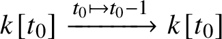
with the morphism of dg-algebras

is given by

. It therefore follows from Lemma 5.3 that for $n=2$
, the pushout square (36) is equivalent to the image under
$n=2$
, the pushout square (36) is equivalent to the image under
of the following homotopy pushout diagram of dg-categories with a single object:

where $k[t_{0},t_{1}]$
denotes the dg-algebra freely generated by
$k[t_{0},t_{1}]$
denotes the dg-algebra freely generated by $t_{0}$
and
$t_{0}$
and $t_{1}$
in degrees
$t_{1}$
in degrees $0$
and
$0$
and $1$
and differential d determined by
$1$
and differential d determined by $d(t_{1})=t_{0}, d(t_{0})=0$
. It follows that there exists an equivalence of k-linear
$d(t_{1})=t_{0}, d(t_{0})=0$
. It follows that there exists an equivalence of k-linear $\infty $
-categories
$\infty $
-categories $\operatorname {Fun}\left (S^{2},\mathcal {D}(k)\right )\simeq \mathcal {D}(k[t_{1}])$
, making the the upper half of diagram (38) commute. The k-linear functors
$\operatorname {Fun}\left (S^{2},\mathcal {D}(k)\right )\simeq \mathcal {D}(k[t_{1}])$
, making the the upper half of diagram (38) commute. The k-linear functors $\phi ^{*}:\mathcal {D}(k)\rightarrow \mathcal {D}(k[t_{1}])$
and
$\phi ^{*}:\mathcal {D}(k)\rightarrow \mathcal {D}(k[t_{1}])$
and $f^{*}:\mathcal {D}(k)\rightarrow \operatorname {Fun}\left (S^{2},\mathcal {D}(k)\right )$
are determined by
$f^{*}:\mathcal {D}(k)\rightarrow \operatorname {Fun}\left (S^{2},\mathcal {D}(k)\right )$
are determined by $\phi ^{*}(k)$
and
$\phi ^{*}(k)$
and $f^{*}(k)$
, respectively. The homology of the chain complex underlying the right
$f^{*}(k)$
, respectively. The homology of the chain complex underlying the right $k[t_{1}]$
-module
$k[t_{1}]$
-module $\phi ^{*}(k)$
is concentrated in degree
$\phi ^{*}(k)$
is concentrated in degree $0$
, given by k. Using the facts that the upper half of diagram (38) commutes and that
$0$
, given by k. Using the facts that the upper half of diagram (38) commutes and that $i^{*}f^{*}(k)=k$
, it follows that
$i^{*}f^{*}(k)=k$
, it follows that $f^{*}(k)$
is also mapped under the equivalence
$f^{*}(k)$
is also mapped under the equivalence $\operatorname {Fun}\left (S^{2},\mathcal {D}(k)\right )\simeq \mathcal {D}(k[t_{1}])$
to a right
$\operatorname {Fun}\left (S^{2},\mathcal {D}(k)\right )\simeq \mathcal {D}(k[t_{1}])$
to a right $k[t_{1}]$
-module with homology k. There exists a unique right
$k[t_{1}]$
-module with homology k. There exists a unique right $k[t_{1}]$
-module, up to quasi-isomorphism, with homology k. This right
$k[t_{1}]$
-module, up to quasi-isomorphism, with homology k. This right $k[t_{1}]$
-module k is equivalent to the module determined by the morphism of dg-algebras
$k[t_{1}]$
-module k is equivalent to the module determined by the morphism of dg-algebras

. It follows that the lower half of diagram (38) commutes for $n=2$
. For
$n=2$
. For $n>3$
, one can argue analogously and by induction. The pushout square (36) is equivalent to the image under
$n>3$
, one can argue analogously and by induction. The pushout square (36) is equivalent to the image under
of the following homotopy pushout diagram of dg-categories:

Here again, $k[t_{n-2},t_{n-1}]$
denotes the freely generated dg-algebra with two generators in degrees
$k[t_{n-2},t_{n-1}]$
denotes the freely generated dg-algebra with two generators in degrees $n-2$
and
$n-2$
and $n-1$
and differential determined by
$n-1$
and differential determined by $d(t_{n-1})=t_{n-2}, d(t_{n-2})=0$
. We find the desired equivalence of k-linear
$d(t_{n-1})=t_{n-2}, d(t_{n-2})=0$
. We find the desired equivalence of k-linear $\infty $
-categories
$\infty $
-categories $\operatorname {Fun}(S^{n},\mathcal {D}(k))\simeq \mathcal {D}(k[t_{n-1}])$
, making the upper half of diagram (38) commute. Showing that the lower half of diagram (38) commutes is analogous to the case
$\operatorname {Fun}(S^{n},\mathcal {D}(k))\simeq \mathcal {D}(k[t_{n-1}])$
, making the upper half of diagram (38) commute. Showing that the lower half of diagram (38) commutes is analogous to the case $n=2$
.
$n=2$
.
Remark 5.6. The composite functor
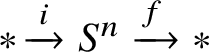
is an equivalence of spaces. The functor

is thus equivalent to $\operatorname {id}_{\mathcal {D}(k)}$
. By the sphericalness of
$\operatorname {id}_{\mathcal {D}(k)}$
. By the sphericalness of $f^{*}\dashv f_{*}$
, there exists an equivalence
$f^{*}\dashv f_{*}$
, there exists an equivalence $f_{*}\simeq f_![-n]$
and therefore
$f_{*}\simeq f_![-n]$
and therefore $f_{*}i_!(k)\simeq k[-n]$
. Note that Proposition 5.5 shows that
$f_{*}i_!(k)\simeq k[-n]$
. Note that Proposition 5.5 shows that $i_!(k)$
is equivalent to the compact generator
$i_!(k)$
is equivalent to the compact generator $k[t_{n-1}]\in \mathcal {D}(k[t_{n-1}])\simeq \operatorname {Fun}(S^{n},\mathcal {D}(k))$
.
$k[t_{n-1}]\in \mathcal {D}(k[t_{n-1}])\simeq \operatorname {Fun}(S^{n},\mathcal {D}(k))$
.
We now describe the cotwist functor $T_{\operatorname {Fun}\left (S^{n},\mathcal {D}(k)\right )}$
of the spherical adjunction
$T_{\operatorname {Fun}\left (S^{n},\mathcal {D}(k)\right )}$
of the spherical adjunction $f^{*}\dashv f_{*}$
for
$f^{*}\dashv f_{*}$
for $n\geq 2$
. Consider the morphism of dg-algebras
$n\geq 2$
. Consider the morphism of dg-algebras $\varphi :k[t_{n-1}]\rightarrow k[t_{n-1}]$
determined by
$\varphi :k[t_{n-1}]\rightarrow k[t_{n-1}]$
determined by $\varphi (t_{n-1})= (-1)^{n-1}t_{n-1}$
. Let
$\varphi (t_{n-1})= (-1)^{n-1}t_{n-1}$
. Let $\varphi ^{*}:\mathcal {D}(k[t_{n-1}])\rightarrow \mathcal {D}(k[t_{n-1}])$
be the pullback functor.
$\varphi ^{*}:\mathcal {D}(k[t_{n-1}])\rightarrow \mathcal {D}(k[t_{n-1}])$
be the pullback functor.
Proposition 5.7. Set $n\geq 2$
and let k be a commutative ring. There exists a commutative diagram in
$n\geq 2$
and let k be a commutative ring. There exists a commutative diagram in $\operatorname {LinCat}_{k}$
as follows:
$\operatorname {LinCat}_{k}$
as follows:

Remark 5.8. Note that only if n is odd does there exist an equivalence of functors $T_{\operatorname {Fun}\left (S^{n},\mathcal {D}(k)\right )}\simeq [-n]$
. The functor
$T_{\operatorname {Fun}\left (S^{n},\mathcal {D}(k)\right )}\simeq [-n]$
. The functor $T_{\operatorname {Fun}\left (S^{n},\mathcal {D}(k)\right )}[n]$
is otherwise the involution reversing the sign of
$T_{\operatorname {Fun}\left (S^{n},\mathcal {D}(k)\right )}[n]$
is otherwise the involution reversing the sign of $t_{n-1}$
.
$t_{n-1}$
.
Proof of Proposition 5.7.
The dg-category of $k[t_{n-1}]$
-bimodules is equivalent to the dg-category
$k[t_{n-1}]$
-bimodules is equivalent to the dg-category $\operatorname {dgMod}(k[t_{n-1}]\otimes _{k} k[t_{n-1}]^{\operatorname {op}})$
. The former dg-category thus inherits a model structure from the projective model structure of the latter, whose underlying
$\operatorname {dgMod}(k[t_{n-1}]\otimes _{k} k[t_{n-1}]^{\operatorname {op}})$
. The former dg-category thus inherits a model structure from the projective model structure of the latter, whose underlying $\infty $
-category is equivalent to the
$\infty $
-category is equivalent to the $\infty $
-category of k-linear endofunctors of
$\infty $
-category of k-linear endofunctors of $\mathcal {D}(k[t_{n-1}])$
. Let
$\mathcal {D}(k[t_{n-1}])$
. Let $\odot $
denote the multiplication in
$\odot $
denote the multiplication in $k[t_{n-1}]$
. We denote by
$k[t_{n-1}]$
. We denote by $\widehat {{k[t_{n-1}]}}$
the
$\widehat {{k[t_{n-1}]}}$
the $k[t_{n-1}]$
-bimodule
$k[t_{n-1}]$
-bimodule $\widehat {{k[t_{n-1}]}}$
with
$\widehat {{k[t_{n-1}]}}$
with
-
• underlying chain complex
$k[t_{n-1}]$
, -
• left action on
$a\in \widehat {k[t_{n-1}]}$
determined by
$t_{n-1}^{i}.a=(-1)^{i(n-1)}t_{n-1}^{i}\odot a$
and -
• right action on
$a\in \widehat {k[t_{n-1}]}$
determined by
$a.t_{n-1}^{i}=a\odot t_{n-1}^{i}$
.


Note that
 . We can thus prove the proposition by showing that the composite of the twist functor $T_{\operatorname {Fun}\left (S^{n},\mathcal {D}(k)\right )}^{\prime }$
of the spherical adjunction
$T_{\operatorname {Fun}\left (S^{n},\mathcal {D}(k)\right )}^{\prime }$
of the spherical adjunction $f_!\dashv f^{*}$
with the equivalence (37) is equivalent to
$f_!\dashv f^{*}$
with the equivalence (37) is equivalent to
 . Using the commutativity of the lower part of diagram (38), it suffices to show that the twist functor T of the spherical adjunction $\phi _!\dashv \phi ^{*}$
is equivalent to
$\phi _!\dashv \phi ^{*}$
is equivalent to
 .
.
Using Remark 5.6, it follows that $\phi ^{*}\phi _!(k[t_{n-1}])\simeq k\in \mathcal {D}(k[t_{n-1}])$
, with k the
$\phi ^{*}\phi _!(k[t_{n-1}])\simeq k\in \mathcal {D}(k[t_{n-1}])$
, with k the $k[t_{n-1}]$
-bimodule determined by the morphism of dg-algebras
$k[t_{n-1}]$
-bimodule determined by the morphism of dg-algebras $\phi $
. The k-linear functor
$\phi $
. The k-linear functor $\phi ^{*}\phi _!$
is thus equivalent to the functor
$\phi ^{*}\phi _!$
is thus equivalent to the functor
, for a $k[t_{n-1}]$
-bimodule k. There is a unique such bimodule, which carries the action
$k[t_{n-1}]$
-bimodule k. There is a unique such bimodule, which carries the action $t_{n-1}.1=0=1.t_{n-1}\in k$
. A cofibrant replacement of the
$t_{n-1}.1=0=1.t_{n-1}\in k$
. A cofibrant replacement of the $k[t_{n-1}]$
-bimodule k is given the cone of the morphism of bimodules
$k[t_{n-1}]$
-bimodule k is given the cone of the morphism of bimodules
 $$ \begin{align*} \alpha:\widehat{k[t_{n-1}]}[n-1]&\rightarrow k[t_{n-1}].,\\ t_{n-1}^{i}&\mapsto t_{n-1}^{i}. \end{align*} $$
To see that $\alpha $
indeed exists, note that by the definition of
$\alpha $
indeed exists, note that by the definition of $\widehat {k[t_{n-1}]}$
and the sign rule for the shift of left modules (see Remark 2.9), the left action of
$\widehat {k[t_{n-1}]}$
and the sign rule for the shift of left modules (see Remark 2.9), the left action of $k[t_{n-1}]$
on
$k[t_{n-1}]$
on $\widehat {k[t_{n-1}]}[n-1]$
is determined by
$\widehat {k[t_{n-1}]}[n-1]$
is determined by $t_{n-1}.1=(-1)^{(n-1)+(n-1)}t_{n-1}=t_{n-1}$
. We deduce that the twist functor T is equivalent to the functor given by tensoring with the homotopy pushout in the following diagram of cofibrant
$t_{n-1}.1=(-1)^{(n-1)+(n-1)}t_{n-1}=t_{n-1}$
. We deduce that the twist functor T is equivalent to the functor given by tensoring with the homotopy pushout in the following diagram of cofibrant $k[t_{n-1}]$
-bimodules:
$k[t_{n-1}]$
-bimodules:

We have shown
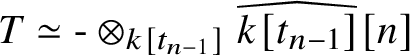
, finishing the proof.
5.2
$\mathcal {V}^{2}_{f^{*}}$
and
$\mathcal {V}^{3}_{f^{*}}$


For $n\geq 2$
, we consider the spherical adjunction
$n\geq 2$
, we consider the spherical adjunction $f^{*}:\mathcal {D}(k)\leftrightarrow \operatorname {Fun}(S^{n},\mathcal {D}(k)):f_{*}$
of Proposition 5.1. The goal of this section is to prove Propositions 5.9 and 5.12, describing the parametrised perverse schober on a
$f^{*}:\mathcal {D}(k)\leftrightarrow \operatorname {Fun}(S^{n},\mathcal {D}(k)):f_{*}$
of Proposition 5.1. The goal of this section is to prove Propositions 5.9 and 5.12, describing the parametrised perverse schober on a $2$
-gon and
$2$
-gon and $3$
-gon obtained from the spherical adjunction
$3$
-gon obtained from the spherical adjunction $f^{*}\dashv f_{*}$
.
$f^{*}\dashv f_{*}$
.
Proposition 5.9. Let k be a commutative ring and set $n\geq 2$
. Let
$n\geq 2$
. Let $D_{2}$
be the freely generated dg-category with two objects
$D_{2}$
be the freely generated dg-category with two objects $x,z$
$x,z$

with morphisms in degrees $\lvert c\rvert =0$
and
$\lvert c\rvert =0$
and $\lvert c^{*}\rvert =n-1$
and vanishing differentials. Further, let
$\lvert c^{*}\rvert =n-1$
and vanishing differentials. Further, let $D_{3}$
be the freely generated dg-category with three objects
$D_{3}$
be the freely generated dg-category with three objects $x,y,z$

with morphisms in degrees $\lvert b\rvert =\lvert c\rvert =0, \lvert a\rvert =n-2, \lvert b^{*}\rvert =\lvert c^{*}\rvert =n-1, \lvert a^{*}\rvert =1$
and differential determined by
$\lvert b\rvert =\lvert c\rvert =0, \lvert a\rvert =n-2, \lvert b^{*}\rvert =\lvert c^{*}\rvert =n-1, \lvert a^{*}\rvert =1$
and differential determined by
 $$ \begin{gather*} d(a)=d(b)=d(c)=0, \\ d(a^{*})=cb, \qquad d(b^{*})=ac, \qquad d(c^{*})=ba. \end{gather*} $$
There exist equivalences of $\infty $
-categories
$\infty $
-categories
 $$ \begin{align} \mathcal{N}_{f^{*}} & \simeq \mathcal{D}(k[t_{n-1}]), \end{align} $$
 $$ \begin{align} \mathcal{V}^{2}_{f^{*}} & \simeq \mathcal{D}(D_{2}), \end{align} $$
 $$ \begin{align} \mathcal{V}^{3}_{f^{*}} &\simeq \mathcal{D}(D_{3}). \end{align} $$
Remark 5.10. Proposition 5.9 shows that dimension $n=2$
is distinguished. Only in dimension
$n=2$
is distinguished. Only in dimension $n=2$
do we find the morphisms
$n=2$
do we find the morphisms $a,b,c$
in
$a,b,c$
in $D_{3}$
to all be in degree
$D_{3}$
to all be in degree $0$
.
$0$
.
Notation 5.11. For $\tau =+,-$
, denote by
$\tau =+,-$
, denote by $i_{1}^{\tau },i_{2}^{\tau },i_{3}^{\tau }:k[t_{n-1}]\rightarrow D_{3}$
the dg-functors determined by mapping
$i_{1}^{\tau },i_{2}^{\tau },i_{3}^{\tau }:k[t_{n-1}]\rightarrow D_{3}$
the dg-functors determined by mapping $\ast $
to
$\ast $
to $x,z,y$
, respectively, and
$x,z,y$
, respectively, and $t_{n-1}$
to
$t_{n-1}$
to $\tau (cc^{*}-a^{*}a), \tau (bb^{*}-c^{*}c), \tau ((-1)^{n}aa^{*}-b^{*}b)$
. We further set
$\tau (cc^{*}-a^{*}a), \tau (bb^{*}-c^{*}c), \tau ((-1)^{n}aa^{*}-b^{*}b)$
. We further set $(-)^{n}=+$
if n is even and
$(-)^{n}=+$
if n is even and $(-)^{n}=-$
if n is odd.
$(-)^{n}=-$
if n is odd.
Proposition 5.12.
-
1. Under the equivalences (39) and (41), the functors
$\varsigma _{2},\varsigma _{3}:\mathcal {N}_{f^{*}}\rightarrow \mathcal {V}^{3}_{f^{*}}$
are equivalent to the image under
of the dg-functors
$i_{2}^{(-)^{n-1}}$
and
$i_{3}^{(-)^{n}}$
, respectively. If
$n=2$
, then
$\varsigma _{1}$
is equivalent to
$\mathcal {D}\left (i_{1}^{+}\right )$
. -
2. Suppose that
$n=2$
. Under the equivalences (39) and (40), the functors
$\varsigma _{1},\varsigma _{2}:\mathcal {N}_{f^{*}}\rightarrow \mathcal {V}^{2}_{f^{*}}$
are equivalent to the image under
of the dg-functors
$k[t_{1}]\rightarrow D_{2}$
determined by mapping
$t_{1}$
to
$cc^{*}$
and
$c^{*}c$
, respectively.


Lemma 5.13. Set $n\geq 2$
.
$n\geq 2$
.
-
1. There exists an equivalence of
$\infty $
-categories (42)where
$$ \begin{align} \mathcal{V}^{2}_{f^{*}}\simeq \mathcal{D}(\bf A_{2}), \end{align} $$
is the upper triangular dg-algebra.
$$ \begin{align*} \bf{A_{2}}=\begin{pmatrix} k & k[-n] \\ 0 & k[t_{n-1}]\end{pmatrix} \end{align*} $$
-
2. There exists an equivalence of
$\infty $
-categories (43)where
$$ \begin{align} \mathcal{V}^{3}_{f^{*}}\simeq \mathcal{D}(\bf A_{3}), \end{align} $$
is the upper triangular dg-algebra.
$$ \begin{align*} \bf{A_{3}}=\begin{pmatrix} k & k[-n] & 0 \\ 0 & k[t_{n-1}] & k[t_{n-1}] \\ 0 & 0 & k[t_{n-1}]\end{pmatrix}\end{align*} $$


Proof. This follows from Proposition 2.39 and the characterisation of $f^{*}$
in Proposition 5.5, as well as Remark 5.6.
$f^{*}$
in Proposition 5.5, as well as Remark 5.6.
Proof of Proposition 5.9.
We have constructed equivalence (39) in Proposition 5.5.
Before we continue with the construction of the equivalences (40) and (41), we collect the following sign rules used implicitly in the following. Let C be any dg-category, set $x,y\in \operatorname {dgMod}(C)$
two dg-modules and consider a morphism
$x,y\in \operatorname {dgMod}(C)$
two dg-modules and consider a morphism $\alpha :x\rightarrow y$
. The cone
$\alpha :x\rightarrow y$
. The cone $\operatorname {cone}(\alpha )=x[1]\oplus y$
has the differential
$\operatorname {cone}(\alpha )=x[1]\oplus y$
has the differential $d_{n}(x,y)=(-d(x),d(y)-\alpha (x))$
. The morphism complex
$d_{n}(x,y)=(-d(x),d(y)-\alpha (x))$
. The morphism complex $\operatorname {Hom}(x,y)$
has differential
$\operatorname {Hom}(x,y)$
has differential $d(f)=d_{y}\circ f - (-1)^{\operatorname {deg}(f)}f\circ d_{x}$
.
$d(f)=d_{y}\circ f - (-1)^{\operatorname {deg}(f)}f\circ d_{x}$
.
We proceed with the construction of equivalence (41).
Consider the compact generators
 $$ \begin{align*} v=p_{1}\textbf{A}_{\textbf{3}}[-n], \qquad y=p_{2}\textbf{A}_{\textbf{3}}, \qquad z=p_{3}\textbf{A}_{\textbf{3}} \end{align*} $$
of $\mathcal {D}(\bf A_{3})$
. Let
$\mathcal {D}(\bf A_{3})$
. Let $w=\operatorname {cone}(e)$
, with e given by
$w=\operatorname {cone}(e)$
, with e given by $1\in k[-n]\simeq \operatorname {Hom}_{\operatorname {dgMod}\left (\bf A_{3}\right )}(v,y)$
. Note that
$1\in k[-n]\simeq \operatorname {Hom}_{\operatorname {dgMod}\left (\bf A_{3}\right )}(v,y)$
. Note that $w,y,z$
are also compact generators of
$w,y,z$
are also compact generators of $\mathcal {D}(\mathbf {A_{3}})$
. A direct inspection shows that the full dg-subcategory
$\mathcal {D}(\mathbf {A_{3}})$
. A direct inspection shows that the full dg-subcategory $\langle w,y,z\rangle \subset \operatorname {dgMod}(\bf A_{3})$
spanned by
$\langle w,y,z\rangle \subset \operatorname {dgMod}(\bf A_{3})$
spanned by $w,y,z$
is quasiequivalent to the dg-category C with objects
$w,y,z$
is quasiequivalent to the dg-category C with objects $w,y,z$
and morphisms generated by the morphisms depicted in
$w,y,z$
and morphisms generated by the morphisms depicted in

in the degrees $\lvert \epsilon \rvert =\lvert \gamma \rvert =0, \lvert t_{z}\rvert =\lvert \eta \rvert =n-1, \lvert \delta \rvert =n$
and with vanishing differentials, subject to the relation
$\lvert \epsilon \rvert =\lvert \gamma \rvert =0, \lvert t_{z}\rvert =\lvert \eta \rvert =n-1, \lvert \delta \rvert =n$
and with vanishing differentials, subject to the relation $t_{z}\circ \gamma =\gamma \circ \epsilon \circ \eta $
. We list the images of the generating morphisms in C under the quasiequivalence
$t_{z}\circ \gamma =\gamma \circ \epsilon \circ \eta $
. We list the images of the generating morphisms in C under the quasiequivalence $C\rightarrow \langle w,y,z\rangle $
.
$C\rightarrow \langle w,y,z\rangle $
.
-
• The morphism
$\epsilon $
maps to
$\left (\operatorname {id}_{y},0\right )\in \operatorname {Hom}(y,y)\oplus \operatorname {Hom}(v[1],y)\simeq \operatorname {Hom}(w,y)$
(the splitting here and in the following neglects the differentials). -
• The morphism
$\eta $
maps to
$t_{n-1}\in k[t_{n-1}]\simeq \operatorname {Hom}(y,y)\subset \operatorname {Hom}(w,y)$
. -
• The morphism
$\gamma $
maps to
$1\in k[t_{n-1}]\simeq \operatorname {Hom}(y,z)\subset \operatorname {Hom}(w,z)$
. -
• The morphism
$t_{z}$
maps to
$t_{n-1}\in k[t_{n-1}]\simeq \operatorname {Hom}(z,z)$
.


We denote by x the cone of $-\gamma :w\rightarrow z$
in
$-\gamma :w\rightarrow z$
in $\operatorname {dgMod}(C)$
and by
$\operatorname {dgMod}(C)$
and by $\langle x,y,z\rangle $
the full dg-subcategory of
$\langle x,y,z\rangle $
the full dg-subcategory of $\operatorname {dgMod}(C)$
spanned by
$\operatorname {dgMod}(C)$
spanned by $x,y,z$
. There exists a quasiequivalence of dg-categories
$x,y,z$
. There exists a quasiequivalence of dg-categories $C^{\prime }\rightarrow \langle x,y,z\rangle $
, where
$C^{\prime }\rightarrow \langle x,y,z\rangle $
, where $C^{\prime }$
is the dg-category with objects
$C^{\prime }$
is the dg-category with objects $x,y,z$
and generating morphisms given by
$x,y,z$
and generating morphisms given by

in the degrees $\lvert a\rvert =n-2, \lvert b\rvert =\lvert c\rvert =0, \lvert a^{*}\rvert =1, \lvert c^{*}\rvert =n-1$
subject to the relation
$\lvert a\rvert =n-2, \lvert b\rvert =\lvert c\rvert =0, \lvert a^{*}\rvert =1, \lvert c^{*}\rvert =n-1$
subject to the relation $ac=0$
. The differentials are determined on the generators by
$ac=0$
. The differentials are determined on the generators by $d(a^{*})=cb$
and
$d(a^{*})=cb$
and $d(c^{*})=ba$
. We collect the images under the dg-functor
$d(c^{*})=ba$
. We collect the images under the dg-functor $C^{\prime }\rightarrow \langle x,y,z\rangle $
of the generating morphisms in
$C^{\prime }\rightarrow \langle x,y,z\rangle $
of the generating morphisms in $C^{\prime }$
.
$C^{\prime }$
.
-
• The morphism b maps to
$\gamma \circ \epsilon $
. -
• The morphism a maps to
$(\eta ,0)\in \operatorname {Hom}_{C}(w[1],y)\oplus \operatorname {Hom}_{C}(z,y)\simeq \operatorname {Hom}_{\langle x,y,z\rangle }(x,y)$
(the splitting again neglects the differentials). -
• The morphism c maps to
$\left (0,\operatorname {id}_{z}\right )\in \operatorname {Hom}_{C}(z,w[1])\oplus \operatorname {Hom}_{C}(z,z)\simeq \operatorname {Hom}_{\langle x,y,z\rangle }(z,x)$
. -
• The morphism
$a^{*}$
maps to
$(\epsilon ,0)\in \operatorname {Hom}_{C}(y,w[1])\oplus \operatorname {Hom}_{C}(y,z)\simeq \operatorname {Hom}_{\langle x,y,z\rangle }(y,x)$
. -
• The morphism
$c^{*}$
maps to
$\left (0,(-1)^{n}t_{z}\right )\in \operatorname {Hom}_{C}(w[1],z)\oplus \operatorname {Hom}_{C}(z,z)\simeq \operatorname {Hom}_{\langle x,y,z\rangle }(x,z)$
.


A direct inspection reveals the homology of the mapping complexes in $C^{\prime }$
:
$C^{\prime }$
:
 $$ \begin{align*} H_{\ast}\operatorname{Hom}_{C^{\prime}}(x,x)&\simeq H_{\ast}\operatorname{Hom}_{C^{\prime}}(y,y)\simeq H_{\ast}\operatorname{Hom}_{C^{\prime}}(z,z)\simeq k[t_{n-1}],\\ H_{\ast}\operatorname{Hom}_{C^{\prime}}(x,y)&\simeq k[t_{n-1}][n-1],\\ H_{\ast}\operatorname{Hom}_{C^{\prime}}(y,z)&\simeq H_{\ast}\operatorname{Hom}_{C^{\prime}}(z,x)\simeq k[t_{n-1}],\\ H_{\ast}\operatorname{Hom}_{C^{\prime}}(x,z)&\simeq H_{\ast}\operatorname{Hom}_{C^{\prime}}(y,x)\simeq H_{\ast}\operatorname{Hom}_{C^{\prime}}(z,y)\simeq 0. \end{align*} $$
We define a dg-functor $\mu :D_{3}\rightarrow C^{\prime }$
by mapping
$\mu :D_{3}\rightarrow C^{\prime }$
by mapping $x,y,z$
to
$x,y,z$
to $x,y,z$
;
$x,y,z$
; $a,b,c$
to
$a,b,c$
to $a,b,c$
; and
$a,b,c$
; and $a^{*},b^{*},c^{*}$
to
$a^{*},b^{*},c^{*}$
to $a^{*},0,c^{*}$
. Lemma 5.14 implies that
$a^{*},0,c^{*}$
. Lemma 5.14 implies that $\mu $
is a quasiequivalence. In total, we obtain equivalences of
$\mu $
is a quasiequivalence. In total, we obtain equivalences of $\infty $
-categories
$\infty $
-categories
 $$ \begin{align*} \mathcal{D}(D_{3})\simeq \mathcal{D}(C^{\prime})\simeq \mathcal{D}(\langle x,y,z\rangle) \simeq \mathcal{D}(C)\simeq \mathcal{D}(\textbf{A}_{\textbf{3}})\overset{\text{formula~}(43)}{\simeq} \mathcal{V}^{3}_{f^{*}}, \end{align*} $$
which yields the desired equivalence (41).
For the construction of equivalence (40), we consider the pushout diagram in $\mathcal {P}r^{L}$

where $\pi _{1,3}$
denotes the projection to the first and third components of the semiorthogonal decomposition. The upper part of the diagram is equivalent to the image under
$\pi _{1,3}$
denotes the projection to the first and third components of the semiorthogonal decomposition. The upper part of the diagram is equivalent to the image under
of the diagram of dg-categories

whose homotopy colimit is easily seen to be quasiequivalent to $D_{2}$
. This observation provides us with the equivalence of
$D_{2}$
. This observation provides us with the equivalence of $\infty $
-categories
$\infty $
-categories $\mathcal {D}(D_{2})\simeq \mathcal {V}^{2}_{f^{*}}$
.
$\mathcal {D}(D_{2})\simeq \mathcal {V}^{2}_{f^{*}}$
.
Lemma 5.14. There exist isomorphisms of graded k-modules
 $$ \begin{align*} H_{\ast}\operatorname{Hom}_{D_{3}}(x,x)&\simeq H_{\ast}\operatorname{Hom}_{D_{3}}(y,y)\simeq H_{\ast}\operatorname{Hom}_{D_{3}}(z,z)\simeq k[t_{n-1}],\\ H_{\ast}\operatorname{Hom}_{D_{3}}(x,y)[1-n]&\simeq H_{\ast}\operatorname{Hom}_{D_{3}}(y,z)\simeq H_{\ast}\operatorname{Hom}_{D_{3}}(z,x)\simeq k[t_{n-1}],\\ H_{\ast}\operatorname{Hom}_{D_{3}}(x,z)&\simeq H_{\ast}\operatorname{Hom}_{D_{3}}(y,x)\simeq H_{\ast}\operatorname{Hom}_{D_{3}}(z,y)\simeq 0. \end{align*} $$
Proof. The morphisms $a,b,c$
and
$a,b,c$
and $a^{*},b^{*},c^{*}$
freely generate
$a^{*},b^{*},c^{*}$
freely generate $D_{3}$
. Any morphism in
$D_{3}$
. Any morphism in $D_{3}$
is thus given by a k-linear sum of composites of these generating morphisms. Given a morphism in
$D_{3}$
is thus given by a k-linear sum of composites of these generating morphisms. Given a morphism in $D_{3}$
, we call the maximal number of generating morphisms appearing in any one of its summands the length of the morphism. We show by induction over the length of a morphism u in
$D_{3}$
, we call the maximal number of generating morphisms appearing in any one of its summands the length of the morphism. We show by induction over the length of a morphism u in $D_{3}$
the following statements:
$D_{3}$
the following statements:
-
i) Any cycle
$u:x\rightarrow x$
(in the morphism complex of
$D_{3}$
) is homologous to
$\lambda (a^{*}a-cc^{*})^{i}$
, with
$\lambda \in k$
and
$i\geq 0$
. -
ii) Any cycle
$u:x\rightarrow y$
is homologous to
$a\circ \lambda (a^{*}a-cc^{*})^{i}$
. -
iii) Any cycle
$u:z\rightarrow y$
is null homologous. -
iv) Further, the previous three statements also hold for
$x,y,z$
, for
$a,b,c$
and for
$a^{*},b^{*},c^{*}$
cyclically permuted (and replacing
$b^{*}b-aa^{*}$
by
$b^{*}b-(-1)^{n-2}aa^{*}$
because of the grading).


The base case is clear. For the induction step, we note that iv) can be shown in the same way as i), ii) and iii) are shown in the following. We begin with i). Consider a cycle $u:x\rightarrow x$
with summands up to a given length. Using the fact that
$u:x\rightarrow x$
with summands up to a given length. Using the fact that $D_{3}$
is freely generated by
$D_{3}$
is freely generated by $a,b,c,a^{*},b^{*},c^{*}$
, we can decompose u into
$a,b,c,a^{*},b^{*},c^{*}$
, we can decompose u into $u=a^{*}u_{1}+cu_{2}$
for two chains
$u=a^{*}u_{1}+cu_{2}$
for two chains $u_{1},u_{2}$
. The condition
$u_{1},u_{2}$
. The condition $d(u)=0$
implies that
$d(u)=0$
implies that $d(u_{1})=0$
. By the induction assumption, we find a chain v satisfying
$d(u_{1})=0$
. By the induction assumption, we find a chain v satisfying $u_{1}=d(v)+a\lambda (a^{*}a-cc^{*})^{i}$
. It follows that u is homologous to the cycle
$u_{1}=d(v)+a\lambda (a^{*}a-cc^{*})^{i}$
. It follows that u is homologous to the cycle
 $$ \begin{align*} u^{\prime}=u+d(a^{*}v)=a^{*}a\lambda(a^{*}a-cc^{*})^{i}+c(u_{2}+bv). \end{align*} $$
From $d(u^{\prime })=0$
it follows that
$d(u^{\prime })=0$
it follows that $d(u_{2}+bv)=-ba\lambda (a^{*}a-cc^{*})^{i}$
. Note that
$d(u_{2}+bv)=-ba\lambda (a^{*}a-cc^{*})^{i}$
. Note that $\lambda (a^{*}a-cc^{*})^{i}$
is not a boundary unless
$\lambda (a^{*}a-cc^{*})^{i}$
is not a boundary unless $\lambda =0$
, in which case u is null homologous. We thus assume that
$\lambda =0$
, in which case u is null homologous. We thus assume that $\lambda \neq 0$
and find that there exists a chain
$\lambda \neq 0$
and find that there exists a chain $v^{\prime }$
with
$v^{\prime }$
with
 $$ \begin{align*} u_{2}+bv= -c^{*}\lambda(a^{*}a-cc^{*})^{i}+v^{\prime}. \end{align*} $$
By the induction assumption it follows that $v^{\prime }$
is a boundary, so we find that u is homologous to
$v^{\prime }$
is a boundary, so we find that u is homologous to $\lambda (aa^{*}-cc^{*})^{i+1}$
, completing the induction step for i).
$\lambda (aa^{*}-cc^{*})^{i+1}$
, completing the induction step for i).
We continue with the induction step for ii). Consider a cycle $u:x\rightarrow y$
. Write
$u:x\rightarrow y$
. Write $u=a\circ u_{1}+b^{*}\circ u_{2}$
for some morphisms
$u=a\circ u_{1}+b^{*}\circ u_{2}$
for some morphisms $u_{1}$
and
$u_{1}$
and $u_{2}$
with
$u_{2}$
with $d(u_{2})=0$
. By the induction assumption we find a chain v with
$d(u_{2})=0$
. By the induction assumption we find a chain v with $u_{2}=d(v)$
. We thus find
$u_{2}=d(v)$
. We thus find
 $$ \begin{align*} u+(-1)^{n}d(b^{*}v)=a\circ u_{1}+(-1)^{n}acv, \end{align*} $$
with $d(u_{1}+(-1)^{n}cv)=0$
. By the induction assumption, we find
$d(u_{1}+(-1)^{n}cv)=0$
. By the induction assumption, we find $u_{1}+(-1)^{n}cv=d(v^{\prime })+\lambda (a^{*}a-cc^{*})^{i}$
, so that
$u_{1}+(-1)^{n}cv=d(v^{\prime })+\lambda (a^{*}a-cc^{*})^{i}$
, so that
 $$ \begin{align*} u+(-1)^{n}d(b^{*}v)-(-1)^{n}d(av^{\prime})=\lambda a\circ (a^{*}a-cc^{*})^{i}, \end{align*} $$
finishing the induction step for ii).
For iii), we consider a cycle $u:z\rightarrow y$
. We decompose u into
$u:z\rightarrow y$
. We decompose u into $u=a\circ u_{1}+ b^{*}\circ u_{2}$
with
$u=a\circ u_{1}+ b^{*}\circ u_{2}$
with $d(u_{2})=0$
. Using the induction assumption we thus find v with
$d(u_{2})=0$
. Using the induction assumption we thus find v with $u_{2}=\lambda (bb^{*}-c^{*}c)^{i}+d(v)$
. It follows that u is homologous to
$u_{2}=\lambda (bb^{*}-c^{*}c)^{i}+d(v)$
. It follows that u is homologous to
 $$ \begin{align*} a\circ (u_{1}+c\circ v)+\lambda b^{*}(bb^{*}-c^{*}c)^{i}. \end{align*} $$
The condition $d(u)=0$
implies that
$d(u)=0$
implies that $(-1)^{n-1}d(u_{1}+c\circ v)=\lambda c(bb^{*}-c^{*}c)^{l}$
. Since
$(-1)^{n-1}d(u_{1}+c\circ v)=\lambda c(bb^{*}-c^{*}c)^{l}$
. Since $c(bb^{*}-c^{*}c)^{l}$
is a nonzero homology class unless
$c(bb^{*}-c^{*}c)^{l}$
is a nonzero homology class unless $\lambda =0$
, we find that
$\lambda =0$
, we find that $\lambda =0$
and
$\lambda =0$
and $d(u_{1}+c\circ v)=0$
. Applying the induction assumption once more, we find that u is homologous to
$d(u_{1}+c\circ v)=0$
. Applying the induction assumption once more, we find that u is homologous to $ac\circ \lambda ^{\prime }(bb^{*}-c^{*}c)^{j}$
, which is the boundary of
$ac\circ \lambda ^{\prime }(bb^{*}-c^{*}c)^{j}$
, which is the boundary of $b^{*}\lambda ^{\prime }(bb^{*}-c^{*}c)^{j}$
. We conclude that u is null homologous, completing the induction step for iii) and the proof.
$b^{*}\lambda ^{\prime }(bb^{*}-c^{*}c)^{j}$
. We conclude that u is null homologous, completing the induction step for iii) and the proof.
Proof of Proposition 5.12.
We begin with the proof of statement $1$
. The functors
$1$
. The functors $\varsigma _{2},\varsigma _{3}[1]:\mathcal {N}_{f^{*}}\rightarrow \mathcal {V}^{3}_{f^{*}}$
are the inclusions of, respectively, the third and second components of the semiorthogonal decomposition of
$\varsigma _{2},\varsigma _{3}[1]:\mathcal {N}_{f^{*}}\rightarrow \mathcal {V}^{3}_{f^{*}}$
are the inclusions of, respectively, the third and second components of the semiorthogonal decomposition of $\mathcal {V}^{3}_{f^{*}}$
. Using Proposition 2.39 and the notation from the proof of Proposition 5.9, we obtain that the functor
$\mathcal {V}^{3}_{f^{*}}$
. Using Proposition 2.39 and the notation from the proof of Proposition 5.9, we obtain that the functor $\varsigma _{2}$
is modelled by the dg-functor
$\varsigma _{2}$
is modelled by the dg-functor $\sigma _{2}:k[t_{n-1}]\rightarrow C^{\prime }$
determined by mapping the unique object
$\sigma _{2}:k[t_{n-1}]\rightarrow C^{\prime }$
determined by mapping the unique object $\ast $
of
$\ast $
of $k[t_{n-1}]$
to z and
$k[t_{n-1}]$
to z and $t_{n-1}$
to
$t_{n-1}$
to $(-1)^{n}c^{*}c$
(the sign arises from the sign of the image of
$(-1)^{n}c^{*}c$
(the sign arises from the sign of the image of $c^{*}$
under the dg-functor
$c^{*}$
under the dg-functor $C^{\prime }\rightarrow \langle x,y,z\rangle $
). Further, let
$C^{\prime }\rightarrow \langle x,y,z\rangle $
). Further, let $\sigma _{2}^{\prime }:k[t_{n-1}]\rightarrow D_{3}$
be the dg-functor determined by mapping
$\sigma _{2}^{\prime }:k[t_{n-1}]\rightarrow D_{3}$
be the dg-functor determined by mapping $\ast $
to z and
$\ast $
to z and $t_{n-1}$
to
$t_{n-1}$
to $(-1)^{n}(c^{*}c-bb^{*})=(-1)^{n-1}(bb^{*}-c^{*}c)$
. The commutative diagram of dg-categories
$(-1)^{n}(c^{*}c-bb^{*})=(-1)^{n-1}(bb^{*}-c^{*}c)$
. The commutative diagram of dg-categories

shows that $\varsigma _{2}$
is also modelled by
$\varsigma _{2}$
is also modelled by $\sigma _{2}^{\prime }$
. An analogous argument shows that
$\sigma _{2}^{\prime }$
. An analogous argument shows that $\varsigma _{3}$
is modelled by the dg-functor
$\varsigma _{3}$
is modelled by the dg-functor $\sigma _{3}:k[t_{n-1}]\rightarrow D_{3}$
determined by mapping
$\sigma _{3}:k[t_{n-1}]\rightarrow D_{3}$
determined by mapping $\ast $
to
$\ast $
to $y^{\prime }$
and
$y^{\prime }$
and $t_{n-1}$
to
$t_{n-1}$
to $aa^{*}-(-1)^{n-2}b^{*}b=(-1)^{n}((-1)^{n}aa^{*}-b^{*}b)$
. In the case that
$aa^{*}-(-1)^{n-2}b^{*}b=(-1)^{n}((-1)^{n}aa^{*}-b^{*}b)$
. In the case that $n=2$
, we can use the sequence of adjunctions
$n=2$
, we can use the sequence of adjunctions
 $$ \begin{align*} \varsigma_{3}\dashv \varrho_{2}\dashv \varsigma_{2}\dashv \varrho_{1}\dashv \varsigma_{1} \end{align*} $$
and the rotational symmetry of $D_{3}$
(which only exists for
$D_{3}$
(which only exists for $n=2$
) to deduce that
$n=2$
) to deduce that $\varsigma _{1}$
is modelled by the dg-functor
$\varsigma _{1}$
is modelled by the dg-functor $k[t_{1}]\rightarrow D_{3}$
determined by mapping
$k[t_{1}]\rightarrow D_{3}$
determined by mapping $\ast $
to
$\ast $
to $x^{\prime }$
and
$x^{\prime }$
and $t_{1}$
to
$t_{1}$
to $(cc^{*}-a^{*}a)$
.
$(cc^{*}-a^{*}a)$
.
We now show statement $2$
. To clarify notation, we denote the right adjoints of the categorified restriction maps
$2$
. To clarify notation, we denote the right adjoints of the categorified restriction maps $\varrho _{1},\varrho _{2}:\mathcal {N}_{f^{*}}\rightarrow \mathcal {V}^{2}_{f^{*}}$
by
$\varrho _{1},\varrho _{2}:\mathcal {N}_{f^{*}}\rightarrow \mathcal {V}^{2}_{f^{*}}$
by $\tilde {\varsigma }_{1}$
and
$\tilde {\varsigma }_{1}$
and $\tilde {\varsigma }_{2}$
, respectively, instead of
$\tilde {\varsigma }_{2}$
, respectively, instead of $\varsigma _{1}$
and
$\varsigma _{1}$
and $\varsigma _{2}$
. We note that there are commutative diagrams in
$\varsigma _{2}$
. We note that there are commutative diagrams in $\mathcal {P}r^{L}$
for
$\mathcal {P}r^{L}$
for $i=1,2$
as follows:
$i=1,2$
as follows:

where $\pi _{1,3}$
denotes the projection to the first and third components of the semiorthogonal decomposition. The functor
$\pi _{1,3}$
denotes the projection to the first and third components of the semiorthogonal decomposition. The functor $\pi _{1,3}$
is modeled by the dg-functor
$\pi _{1,3}$
is modeled by the dg-functor $D_{3}\rightarrow D_{2}$
given by mapping
$D_{3}\rightarrow D_{2}$
given by mapping $x,z$
to
$x,z$
to $x,z$
and
$x,z$
and $c,c^{*}$
to
$c,c^{*}$
to $c,c^{*}$
and all other morphisms to zero. The desired models for
$c,c^{*}$
and all other morphisms to zero. The desired models for $\tilde {\varsigma }_{1}$
and
$\tilde {\varsigma }_{1}$
and $\tilde {\varsigma }_{2}$
thus follow from the models for
$\tilde {\varsigma }_{2}$
thus follow from the models for $\varsigma _{1}$
and
$\varsigma _{1}$
and $\varsigma _{2}$
.
$\varsigma _{2}$
.
6 Gluing Ginzburg algebras via perverse schobers
6.1 The main result
We fix a commutative ring k. Given an ideal triangulation $\mathcal {T}$
of an oriented marked surface, we defined the relative Ginzburg algebra
$\mathcal {T}$
of an oriented marked surface, we defined the relative Ginzburg algebra $\mathscr {G}_{\mathcal {T}}$
in Section 1.1. Consider also the dual ribbon graph
$\mathscr {G}_{\mathcal {T}}$
in Section 1.1. Consider also the dual ribbon graph $\Gamma _{\mathcal {T}}$
of
$\Gamma _{\mathcal {T}}$
of $\mathcal {T}$
of Definition 4.10. In this section we construct a
$\mathcal {T}$
of Definition 4.10. In this section we construct a $\Gamma _{\mathcal {T}}$
-parametrised perverse schober
$\Gamma _{\mathcal {T}}$
-parametrised perverse schober $\mathcal {F}_{\mathcal {T}}$
with the property that the spherical adjunction at each vertex is given by
$\mathcal {F}_{\mathcal {T}}$
with the property that the spherical adjunction at each vertex is given by $f^{*}:\mathcal {D}(k)\leftrightarrow \operatorname {Fun}\left (S^{2},\mathcal {D}(k)\right ):f_{*}$
and whose
$f^{*}:\mathcal {D}(k)\leftrightarrow \operatorname {Fun}\left (S^{2},\mathcal {D}(k)\right ):f_{*}$
and whose $\infty $
-category
$\infty $
-category $\mathcal {H}(\Gamma _{\mathcal {T}},\mathcal {F}_{\mathcal {T}})$
of global sections is equivalent to the derived
$\mathcal {H}(\Gamma _{\mathcal {T}},\mathcal {F}_{\mathcal {T}})$
of global sections is equivalent to the derived $\infty $
-category of the relative Ginzburg algebra
$\infty $
-category of the relative Ginzburg algebra $\mathscr {G}_{\mathcal {T}}$
. As we show in the proof of Theorem 6.1, we can achieve this by making for each vertex of
$\mathscr {G}_{\mathcal {T}}$
. As we show in the proof of Theorem 6.1, we can achieve this by making for each vertex of $\Gamma _{\mathcal {T}}$
a choice of total order of the half-edges at the vertex compatible with the given cyclic order and then defining
$\Gamma _{\mathcal {T}}$
a choice of total order of the half-edges at the vertex compatible with the given cyclic order and then defining $\mathcal {F}_{\mathcal {T}}$
via a gluing of the local model of a parametrised perverse schober from Definition 3.4. To match the signs in the differential of the Ginzburg algebra, some care is required in the choices of the gluing diagrams. This construction depends on the choices of total orders. However, we discuss in Section 7.1 an interpretation of all involved choices in terms of spin structures on the surface without the interior marked points
$\mathcal {F}_{\mathcal {T}}$
via a gluing of the local model of a parametrised perverse schober from Definition 3.4. To match the signs in the differential of the Ginzburg algebra, some care is required in the choices of the gluing diagrams. This construction depends on the choices of total orders. However, we discuss in Section 7.1 an interpretation of all involved choices in terms of spin structures on the surface without the interior marked points $\Sigma =\mathbf {S}\backslash (M\cap \mathbf {S}^{\circ })$
, as well as why the resulting parametrised perverse schober is, up to equivalence, independent of the choices made.
$\Sigma =\mathbf {S}\backslash (M\cap \mathbf {S}^{\circ })$
, as well as why the resulting parametrised perverse schober is, up to equivalence, independent of the choices made.
Theorem 6.1. Let $\mathcal {T}$
be an ideal triangulation of an oriented marked surface. There exists a
$\mathcal {T}$
be an ideal triangulation of an oriented marked surface. There exists a $\Gamma _{\mathcal {T}}$
-parametrised perverse schober
$\Gamma _{\mathcal {T}}$
-parametrised perverse schober $\mathcal {F}_{\mathcal {T}}$
and an equivalence of
$\mathcal {F}_{\mathcal {T}}$
and an equivalence of $\infty $
-categories
$\infty $
-categories
 $$ \begin{align*} \mathcal{H}(\Gamma_{\mathcal{T}},\mathcal{F}_{\mathcal{T}})\simeq \mathcal{D}(\mathscr{G}_{\mathcal{T}}). \end{align*} $$
From Theorem 6.1 we deduce the following:
Corollary 6.2. Let $\mathcal {T}~$
be an ideal triangulation of an oriented marked surface and let
$\mathcal {T}~$
be an ideal triangulation of an oriented marked surface and let $\Gamma _{\mathcal {T}}^{\circ }~$
be the ribbon graph obtained from
$\Gamma _{\mathcal {T}}^{\circ }~$
be the ribbon graph obtained from $\Gamma _{\mathcal {T}}~$
by removing all external edges. Consider the associated quiver
$\Gamma _{\mathcal {T}}~$
by removing all external edges. Consider the associated quiver $Q_{\mathcal {T}}^{\circ }~$
with
$Q_{\mathcal {T}}^{\circ }~$
with $3$
-cyclic potential
$3$
-cyclic potential $W^{\prime }_{\mathcal {T}}$
containing a
$W^{\prime }_{\mathcal {T}}$
containing a $3$
-cycle for each interior ideal triangle of
$3$
-cycle for each interior ideal triangle of $\mathcal {T}$
from Section 1.1. There exists an equivalence of
$\mathcal {T}$
from Section 1.1. There exists an equivalence of $\infty $
-categories
$\infty $
-categories
 $$ \begin{align*} \mathcal{H}_{\Gamma_{\mathcal{T}}^{\circ}}(\Gamma_{\mathcal{T}},\mathcal{F}_{\mathcal{T}}) \simeq \mathcal{D}\left(\mathscr{G}\left(Q_{\mathcal{T}}^{\circ},W^{\prime}_{\mathcal{T}}\right)\right). \end{align*} $$
Proof of Theorem 6.1.
We prove the statement by an induction on the number of ideal triangles of $\mathcal {T}$
and a comparison of the computation of
$\mathcal {T}$
and a comparison of the computation of $\mathcal {H}(\Gamma _{\mathcal {T}},\mathcal {F}_{\mathcal {T}})$
with an explicit computation of homotopy colimits in
$\mathcal {H}(\Gamma _{\mathcal {T}},\mathcal {F}_{\mathcal {T}})$
with an explicit computation of homotopy colimits in $\operatorname {dgCat}_{k}$
with the quasiequivalence model structure.
$\operatorname {dgCat}_{k}$
with the quasiequivalence model structure.
We define a dg-category $C_{\mathcal {T}}$
with objects the vertices of
$C_{\mathcal {T}}$
with objects the vertices of $Q_{\mathcal {T}}$
and morphisms freely generated by the graded arrows of
$Q_{\mathcal {T}}$
and morphisms freely generated by the graded arrows of $\tilde {Q}_{\mathcal {T}}$
(see Section 1.1), and two further endomorphisms
$\tilde {Q}_{\mathcal {T}}$
(see Section 1.1), and two further endomorphisms $l_{e,1}^{\prime },l_{e,2}^{\prime }$
of degrees
$l_{e,1}^{\prime },l_{e,2}^{\prime }$
of degrees $1,2$
at each vertex given by a boundary edge e. To clarify notation, we denote in this proof the degree
$1,2$
at each vertex given by a boundary edge e. To clarify notation, we denote in this proof the degree $2$
loop
$2$
loop $l_{e}:e\rightarrow e$
for
$l_{e}:e\rightarrow e$
for $e\in (Q_{\mathcal {T}})_{0}$
by
$e\in (Q_{\mathcal {T}})_{0}$
by $l_{e,2}$
. The differential d of the morphism complexes is determined on the generators. It acts nontrivially on the generators
$l_{e,2}$
. The differential d of the morphism complexes is determined on the generators. It acts nontrivially on the generators $l_{e,2}^{\prime }$
,
$l_{e,2}^{\prime }$
, $l_{e,2}$
and
$l_{e,2}$
and $a^{*}_{p,i}$
; on the latter two it acts as the differential of
$a^{*}_{p,i}$
; on the latter two it acts as the differential of $\mathscr {G}_{\mathcal {T}}$
, and on
$\mathscr {G}_{\mathcal {T}}$
, and on $l_{e,2}^{\prime }$
it acts as
$l_{e,2}^{\prime }$
it acts as
 $$ \begin{align*} l_{e,2}^{\prime}\mapsto l_{e,1}^{\prime}-\sum_{a\in \left(Q_{\mathcal{T}}\right)_{1}} p_{e}[a,a^{*}]p_{e}. \end{align*} $$
Note that the dg-category $C_{\mathcal {T}}$
is Morita equivalent to
$C_{\mathcal {T}}$
is Morita equivalent to $\mathscr {G}_{\mathcal {T}}$
. For each vertex e corresponding to a boundary edge, we denote by
$\mathscr {G}_{\mathcal {T}}$
. For each vertex e corresponding to a boundary edge, we denote by $i_{e}^{+},i_{e}^{-}:k[t_{1}]\rightarrow C_{\mathcal {T}}$
the dg-functors determined by mapping the unique vertex
$i_{e}^{+},i_{e}^{-}:k[t_{1}]\rightarrow C_{\mathcal {T}}$
the dg-functors determined by mapping the unique vertex $\ast $
of
$\ast $
of $k[t_{1}]$
to
$k[t_{1}]$
to $e\in C_{\mathcal {T}}$
and the generator
$e\in C_{\mathcal {T}}$
and the generator $t_{1}$
to
$t_{1}$
to $l_{e,1}^{\prime }$
and
$l_{e,1}^{\prime }$
and $-l_{e,1}^{\prime }$
, respectively.
$-l_{e,1}^{\prime }$
, respectively.
We deduce the theorem from the following statements, which we prove by an induction on the number of ideal triangles of $\mathcal {T}$
:
$\mathcal {T}$
:
Let $\mathcal {T}~$
be an ideal triangulation of an oriented marked surface with dual ribbon graph
$\mathcal {T}~$
be an ideal triangulation of an oriented marked surface with dual ribbon graph $\Gamma _{\mathcal {T}}$
. There exists a
$\Gamma _{\mathcal {T}}$
. There exists a $\Gamma _{\mathcal {T}}$
-parametrised perverse schober
$\Gamma _{\mathcal {T}}$
-parametrised perverse schober $\mathcal {F}_{\mathcal {T}}~$
with the following properties:
$\mathcal {F}_{\mathcal {T}}~$
with the following properties:
-
1. There exists an equivalence of
$\infty $
-categories
$$ \begin{align*} \mathcal{H}(\Gamma_{\mathcal{T}},\mathcal{F}_{\mathcal{T}})\simeq \mathcal{D}(C_{\mathcal{T}}). \end{align*} $$
-
2. For each boundary edge e of
$\mathcal {T}$
, we denote by
$\operatorname {ev}_{e}:\mathcal {H}(\Gamma _{\mathcal {T}},\mathcal {F}_{\mathcal {T}})\rightarrow \mathcal {F}_{\mathcal {T}}(e)$
the evaluation functor at
$e\in \operatorname {Exit}(\mathcal {T}\;)$
. The left adjoint of the functor (44)is equivalent to
$\mathcal {D}\left (i_{e}^{+}\right )$
or
$\mathcal {D}\left (i_{e}^{-}\right )$
.


In the following we will refer to functor (44) also as the evaluation functor.
Base case of the induction
Let $\mathcal {T}_{1}$
be the ideal triangulation consisting of a single ideal triangle that is not self-folded. We choose a total order on the edges of
$\mathcal {T}_{1}$
be the ideal triangulation consisting of a single ideal triangle that is not self-folded. We choose a total order on the edges of $\mathcal {T}_{1}$
compatible with the cyclic order induced by the anticlockwise orientation. This provides us with an equivalence of posets
$\mathcal {T}_{1}$
compatible with the cyclic order induced by the anticlockwise orientation. This provides us with an equivalence of posets $\operatorname {Exit}\left (\Gamma _{\mathcal {T}_{1}}\right )\simeq C_{3}$
. We can thus define
$\operatorname {Exit}\left (\Gamma _{\mathcal {T}_{1}}\right )\simeq C_{3}$
. We can thus define $\mathcal {F}_{\mathcal {T}_{1}}$
as the parametrised perverse schober
$\mathcal {F}_{\mathcal {T}_{1}}$
as the parametrised perverse schober $\mathcal {G}_{3}(f^{*})$
described in Definition 3.4 corresponding to the spherical adjunction
$\mathcal {G}_{3}(f^{*})$
described in Definition 3.4 corresponding to the spherical adjunction $f^{*}\dashv f_{*}$
(with
$f^{*}\dashv f_{*}$
(with $n=2$
). The existence of the desired equivalence
$n=2$
). The existence of the desired equivalence $\mathcal {H}\left (\mathcal {T}_{1},\mathcal {F}_{\mathcal {T}_{1}}\right )\simeq \mathcal {D}\left (C_{\mathcal {T}_{1}}\right )$
is shown in Propositions 5.9 and 5.12.
$\mathcal {H}\left (\mathcal {T}_{1},\mathcal {F}_{\mathcal {T}_{1}}\right )\simeq \mathcal {D}\left (C_{\mathcal {T}_{1}}\right )$
is shown in Propositions 5.9 and 5.12.
Let now $\mathcal {T}_{1}$
be the ideal triangulation consisting of a single self-folded triangle. We define
$\mathcal {T}_{1}$
be the ideal triangulation consisting of a single self-folded triangle. We define $\mathcal {F}_{\mathcal {T}_{1}}$
using Notation 4.16 as follows:
$\mathcal {F}_{\mathcal {T}_{1}}$
using Notation 4.16 as follows:

The limit $\mathcal {H}\left (\Gamma _{\mathcal {T}_{1}},\mathcal {F}_{\mathcal {T}_{1}}\right )$
is equivalent to the colimit of the left dual
$\mathcal {H}\left (\Gamma _{\mathcal {T}_{1}},\mathcal {F}_{\mathcal {T}_{1}}\right )$
is equivalent to the colimit of the left dual $\underset {\mathcal {P}r^{L}}{\operatorname {colim}} \mathbb {D}^{L} \mathcal {F}_{\mathcal {T}_{1}}$
, which is equivalent to the following coequaliser in
$\underset {\mathcal {P}r^{L}}{\operatorname {colim}} \mathbb {D}^{L} \mathcal {F}_{\mathcal {T}_{1}}$
, which is equivalent to the following coequaliser in $\mathcal {P}r^{L}$
, where
$\mathcal {P}r^{L}$
, where $T=T_{\operatorname {Fun}\left (S^{2},\mathcal {D}(k)\right )}[2]$
denotes the suspension of the cotwist functor of the spherical adjunction
$T=T_{\operatorname {Fun}\left (S^{2},\mathcal {D}(k)\right )}[2]$
denotes the suspension of the cotwist functor of the spherical adjunction $f^{*}\dashv f_{*}$
, also described in Proposition 5.7:
$f^{*}\dashv f_{*}$
, also described in Proposition 5.7:

The colimit of formula (46) is in turn equivalent to the pushout of the following span in $\mathcal {P}r^{L}$
:
$\mathcal {P}r^{L}$
:

Let $\mathcal {T}^{\;\prime }$
be the ideal triangulation consisting of a single ideal triangle, not self-folded, and denote by
$\mathcal {T}^{\;\prime }$
be the ideal triangulation consisting of a single ideal triangle, not self-folded, and denote by $e_{1},e_{3}$
two boundary edges of
$e_{1},e_{3}$
two boundary edges of $\mathcal {T}^{\;\prime }$
. Diagram (47) is equivalent to the image under
$\mathcal {T}^{\;\prime }$
. Diagram (47) is equivalent to the image under
of the following diagram in $\operatorname {dgCat}_{k}$
:
$\operatorname {dgCat}_{k}$
:

The morphism $i_{e_{3}}^{+}\amalg i_{e_{1}}^{-}$
in diagram (48) is a cofibration, and we can thus compute the homotopy colimit of the diagram as the (ordinary) colimit in the
$i_{e_{3}}^{+}\amalg i_{e_{1}}^{-}$
in diagram (48) is a cofibration, and we can thus compute the homotopy colimit of the diagram as the (ordinary) colimit in the $1$
-category of k-linear dg-categories. This colimit is quasiequivalent to
$1$
-category of k-linear dg-categories. This colimit is quasiequivalent to $C_{\mathcal {T}_{1}}$
, showing the desired equivalence
$C_{\mathcal {T}_{1}}$
, showing the desired equivalence $\mathcal {H}\left (\Gamma _{\mathcal {T}_{1}},\mathcal {F}_{\mathcal {T}_{1}}\right )\simeq \mathcal {D}\left (C_{\mathcal {T}_{1}}\right )$
. The left adjoint of the evaluation functor
$\mathcal {H}\left (\Gamma _{\mathcal {T}_{1}},\mathcal {F}_{\mathcal {T}_{1}}\right )\simeq \mathcal {D}\left (C_{\mathcal {T}_{1}}\right )$
. The left adjoint of the evaluation functor $\mathcal {D}\left (C_{\mathcal {T}_{1}}\right )\rightarrow \mathcal {D}(k[t_{1}])$
to e factors as
$\mathcal {D}\left (C_{\mathcal {T}_{1}}\right )\rightarrow \mathcal {D}(k[t_{1}])$
to e factors as

where $e_{2}\neq e_{1},e_{3}$
is the remaining boundary edge of
$e_{2}\neq e_{1},e_{3}$
is the remaining boundary edge of $\mathcal {T}^{\;\prime }$
, and is thus equivalent to
$\mathcal {T}^{\;\prime }$
, and is thus equivalent to $\mathcal {D}\left (i_{e}^{-}\right )$
. This completes the base case of the induction, where the ideal triangulation consists of a single ideal triangle.
$\mathcal {D}\left (i_{e}^{-}\right )$
. This completes the base case of the induction, where the ideal triangulation consists of a single ideal triangle.
Induction step
Assume now that the statement has been shown for all ideal triangulations with at most n ideal triangles. Let $\mathcal {T}_{n+1}$
be an ideal triangulation with
$\mathcal {T}_{n+1}$
be an ideal triangulation with $n+1$
ideal triangles. We choose any subtriangulation
$n+1$
ideal triangles. We choose any subtriangulation $\mathcal {T}_{n}$
consisting of n connected ideal triangles of
$\mathcal {T}_{n}$
consisting of n connected ideal triangles of $\mathcal {T}_{n+1}$
. The complement of
$\mathcal {T}_{n+1}$
. The complement of $\mathcal {T}_{n}$
in
$\mathcal {T}_{n}$
in $\mathcal {T}_{n+1}$
consists of a single ideal triangle and is denoted by
$\mathcal {T}_{n+1}$
consists of a single ideal triangle and is denoted by $\mathcal {T}_{1}$
. Denote by S the set of edges along which
$\mathcal {T}_{1}$
. Denote by S the set of edges along which $\mathcal {T}_{1}$
and
$\mathcal {T}_{1}$
and $\mathcal {T}_{n}$
are glued in
$\mathcal {T}_{n}$
are glued in $\mathcal {T}_{n+1}$
and
$\mathcal {T}_{n+1}$
and $s=\lvert S\rvert $
. To define the
$s=\lvert S\rvert $
. To define the $\Gamma _{\mathcal {T}_{n+1}}$
-parametrised perverse schober
$\Gamma _{\mathcal {T}_{n+1}}$
-parametrised perverse schober $\mathcal {F}_{\mathcal {T}_{n+1}}$
, we wish to glue
$\mathcal {F}_{\mathcal {T}_{n+1}}$
, we wish to glue $\mathcal {F}_{\mathcal {T}_{1}}$
and
$\mathcal {F}_{\mathcal {T}_{1}}$
and $\mathcal {F}_{\mathcal {T}_{n}}$
in the sense of Lemma 4.18. First, however, we modify the diagram
$\mathcal {F}_{\mathcal {T}_{n}}$
in the sense of Lemma 4.18. First, however, we modify the diagram $\mathcal {F}_{\mathcal {T}_{n}}:\operatorname {Exit}\left (\Gamma _{\mathcal {T}_{n}}\right )\rightarrow \operatorname {St}$
by postcomposing the functor
$\mathcal {F}_{\mathcal {T}_{n}}:\operatorname {Exit}\left (\Gamma _{\mathcal {T}_{n}}\right )\rightarrow \operatorname {St}$
by postcomposing the functor
, for each edge $v\rightarrow e$
in
$v\rightarrow e$
in $\operatorname {Exit}\left (\Gamma _{\mathcal {T}_{n}}\right )$
with
$\operatorname {Exit}\left (\Gamma _{\mathcal {T}_{n}}\right )$
with $e\in S$
, with an autoequivalence
$e\in S$
, with an autoequivalence $T_{e}$
of
$T_{e}$
of $\operatorname {Fun}\left (S^{2},\mathcal {D}(k)\right )$
described as follows. Consider the left adjoints of
$\operatorname {Fun}\left (S^{2},\mathcal {D}(k)\right )$
described as follows. Consider the left adjoints of

and

The induction assumption implies that these two left adjoint are each equivalent to either $\mathcal {D}\left (i^{+}_{e}\right )$
or
$\mathcal {D}\left (i^{+}_{e}\right )$
or $\mathcal {D}\left (i^{-}_{e}\right )$
(abusing notation). If both superscripts in this description are identical, each
$\mathcal {D}\left (i^{-}_{e}\right )$
(abusing notation). If both superscripts in this description are identical, each $+$
or
$+$
or $-$
, we choose
$-$
, we choose $T_{e}=T$
, where T is as in the base case of the induction; otherwise we choose
$T_{e}=T$
, where T is as in the base case of the induction; otherwise we choose $T_{e}=\operatorname {id}_{\operatorname {Fun}\left (S^{2},\mathcal {D}(k)\right )}$
. We denote the
$T_{e}=\operatorname {id}_{\operatorname {Fun}\left (S^{2},\mathcal {D}(k)\right )}$
. We denote the $\Gamma _{\mathcal {T}_{n}}$
-parametrised perverse schober obtained from the modification of
$\Gamma _{\mathcal {T}_{n}}$
-parametrised perverse schober obtained from the modification of $\mathcal {F}_{\mathcal {T}_{n}}$
by
$\mathcal {F}_{\mathcal {T}_{n}}$
by $\mathcal {F}^{\;\ast }_{\mathcal {T}_{n}}$
. We define
$\mathcal {F}^{\;\ast }_{\mathcal {T}_{n}}$
. We define $\mathcal {F}_{\mathcal {T}_{n+1}}$
as the gluing of
$\mathcal {F}_{\mathcal {T}_{n+1}}$
as the gluing of $\mathcal {F}_{\mathcal {T}_{1}}$
and
$\mathcal {F}_{\mathcal {T}_{1}}$
and $\mathcal {F}^{\;\ast }_{\mathcal {T}_{n}}$
.
$\mathcal {F}^{\;\ast }_{\mathcal {T}_{n}}$
.
We observe that $\mathcal {H}\left (\Gamma _{\mathcal {T}_{n}}, \mathcal {F}^{\;\ast }_{\mathcal {T}_{n}}\right ) \simeq \mathcal {H}\left (\Gamma _{\mathcal {T}_{n}},\mathcal {F}_{\mathcal {T}_{n}}\right )$
. Using the induction assumption, we thus find equivalences of
$\mathcal {H}\left (\Gamma _{\mathcal {T}_{n}}, \mathcal {F}^{\;\ast }_{\mathcal {T}_{n}}\right ) \simeq \mathcal {H}\left (\Gamma _{\mathcal {T}_{n}},\mathcal {F}_{\mathcal {T}_{n}}\right )$
. Using the induction assumption, we thus find equivalences of $\infty $
-categories
$\infty $
-categories
 $$ \begin{align*} \mathcal{H}\left(\Gamma_{\mathcal{T}_{n}},\mathcal{F}_{\mathcal{T}_{n+1}}\rvert_{\operatorname{Exit}\left(\Gamma_{\mathcal{T}_{n}}\right)}\right)&=\mathcal{H}\left(\Gamma_{\mathcal{T}_{n}},\mathcal{F}^{\;\ast}_{\mathcal{T}_{n}}\right)\simeq \mathcal{D}\left(C_{\mathcal{T}_{n}}\right),\\ \mathcal{H}\left(\Gamma_{\mathcal{T}_{1}},\mathcal{F}_{\mathcal{T}_{n+1}}\rvert_{\operatorname{Exit}\left(\Gamma_{\mathcal{T}_{1}}\right)}\right)&=\mathcal{H}\left(\Gamma_{\mathcal{T}_{1}},\mathcal{F}_{\mathcal{T}_{1}}\right)\simeq \mathcal{D}\left(C_{\mathcal{T}_{1}}\right). \end{align*} $$
A standard result on the decomposition results of colimits [Reference LurieLur09, 4.2.3.10] shows that global sections commute with gluing in the sense that there is a pullback diagram in $\mathcal {P}r^{L}$
as follows:
$\mathcal {P}r^{L}$
as follows:

The left adjoint diagram is equivalent to the image under
of the following homotopy pushout diagram in $\operatorname {dgCat}_{k}$
:
$\operatorname {dgCat}_{k}$
:

The dg-functors $\alpha _{1}$
and
$\alpha _{1}$
and $\alpha _{n}$
each restrict on the component of
$\alpha _{n}$
each restrict on the component of $k[t_{1}]^{\amalg s}$
indexed by a given edge
$k[t_{1}]^{\amalg s}$
indexed by a given edge $e\in S$
to a dg-functor of the form
$e\in S$
to a dg-functor of the form $i_{e}^{+}$
or
$i_{e}^{+}$
or $i_{e}^{-}$
(again by abuse of notation); we denote these functors by
$i_{e}^{-}$
(again by abuse of notation); we denote these functors by $i_{e}^{1}$
and
$i_{e}^{1}$
and $i_{e}^{n}$
, respectively. We will show that
$i_{e}^{n}$
, respectively. We will show that $\alpha _{1}$
and
$\alpha _{1}$
and $\alpha _{n}$
are cofibrations. Diagram (49) is thus also pushout, and we find C to be given as follows. The number of objects of C is
$\alpha _{n}$
are cofibrations. Diagram (49) is thus also pushout, and we find C to be given as follows. The number of objects of C is $\left \lvert \left (Q_{\mathcal {T}_{n}}\right )_{0}\right \rvert + \left \lvert \left (Q_{\mathcal {T}_{1}}\right )_{0}\right \rvert -s$
. The morphisms are freely generated by the edges of
$\left \lvert \left (Q_{\mathcal {T}_{n}}\right )_{0}\right \rvert + \left \lvert \left (Q_{\mathcal {T}_{1}}\right )_{0}\right \rvert -s$
. The morphisms are freely generated by the edges of $Q_{\mathcal {T}_{n}}$
, the edges of
$Q_{\mathcal {T}_{n}}$
, the edges of $Q_{\mathcal {T}_{1}}$
and, for each edge
$Q_{\mathcal {T}_{1}}$
and, for each edge $e\in S$
, two endomorphisms
$e\in S$
, two endomorphisms $\left (l_{e,2}^{\prime }\right )^{1},\left (l_{e,2}^{\prime }\right )^{n}:e\rightarrow e$
in degree
$\left (l_{e,2}^{\prime }\right )^{1},\left (l_{e,2}^{\prime }\right )^{n}:e\rightarrow e$
in degree $2$
and one endomorphism
$2$
and one endomorphism $l_{e,1}^{\prime }:e\rightarrow e$
in degree
$l_{e,1}^{\prime }:e\rightarrow e$
in degree $1$
satisfying
$1$
satisfying
 $$ \begin{align*} d\left(\left(l_{e,2}^{\prime}\right)^{1}\right)=i_{e}^{1}(t_{1})-\sum_{a\in \left(Q_{\mathcal{T}_{1}}\right)_{1}} p_{e}[a,a^{*}]p_{e} \end{align*} $$
and
 $$ \begin{align*} d\left(\left(l_{e,2}^{\prime}\right)^{n}\right)=i_{e}^{n}(t_{1})-\sum_{a\in \left(Q_{\mathcal{T}_{n}}\right)_{1}} p_{e}[a,a^{*}]p_{e}. \end{align*} $$
This choice of $T_{e}$
ensures that
$T_{e}$
ensures that $i_{e}^{1}(t_{1})=-i_{e}^{n}(t_{1})=\pm l_{e,1}^{\prime }$
, and it follows that
$i_{e}^{1}(t_{1})=-i_{e}^{n}(t_{1})=\pm l_{e,1}^{\prime }$
, and it follows that
 $$ \begin{align*} d\left(-\left(l_{e,2}^{\prime}\right)^{1}-\left(l_{e,2}^{\prime}\right)^{n}\right)=\sum_{a\in \left(Q_{\mathcal{T}_{n+1}}\right)_{1}} p_{e}[a,a^{*}]p_{e} \end{align*} $$
is a boundary. We deduce the existence of a quasiequivalence $C_{\mathcal {T}_{n+1}}\rightarrow C$
mapping
$C_{\mathcal {T}_{n+1}}\rightarrow C$
mapping $l_{e,2}$
to
$l_{e,2}$
to $-\left (l_{e,2}^{\prime }\right )^{1}-\left (l_{e,2}^{\prime }\right )^{n}$
. This shows the first part of the induction step.
$-\left (l_{e,2}^{\prime }\right )^{1}-\left (l_{e,2}^{\prime }\right )^{n}$
. This shows the first part of the induction step.
Let e be a boundary edge of ${\mathcal {T}_{n+1}}$
. Assume that it lies in
${\mathcal {T}_{n+1}}$
. Assume that it lies in $\mathcal {T}_{n}$
. The left adjoint of the evaluation functor to e factors as
$\mathcal {T}_{n}$
. The left adjoint of the evaluation functor to e factors as

and thus is equivalent to $\mathcal {D}\left (i_{e}^{\pm }\right )$
. If e lies in
$\mathcal {D}\left (i_{e}^{\pm }\right )$
. If e lies in $\mathcal {T}_{1}$
, we can argue analogously. This shows the second part of the induction step, completing the induction.
$\mathcal {T}_{1}$
, we can argue analogously. This shows the second part of the induction step, completing the induction. $\alpha _{1}$
and
$\alpha _{1}$
and $\alpha _{n}$
are cofibrations
$\alpha _{n}$
are cofibrations
To see that $\alpha _{1}$
is a cofibration, one can directly check the lifting property with respect to the fibrations in the quasiequivalence model structure. To see that
$\alpha _{1}$
is a cofibration, one can directly check the lifting property with respect to the fibrations in the quasiequivalence model structure. To see that $\alpha _{n}$
is a cofibration, we argue by induction on n and decompose
$\alpha _{n}$
is a cofibration, we argue by induction on n and decompose $\mathcal {T}_{n}$
into two ideal triangulations
$\mathcal {T}_{n}$
into two ideal triangulations $\mathcal {T}_{i},\mathcal {T}_{j}$
with
$\mathcal {T}_{i},\mathcal {T}_{j}$
with $i,j<n$
such that
$i,j<n$
such that $\mathcal {T}_{n}$
is obtained by gluing
$\mathcal {T}_{n}$
is obtained by gluing $\mathcal {T}_{i}$
and
$\mathcal {T}_{i}$
and $\mathcal {T}_{j}$
along q edges. One then finds the following commutative diagram in
$\mathcal {T}_{j}$
along q edges. One then finds the following commutative diagram in $\operatorname {dgCat}_{k}$
:
$\operatorname {dgCat}_{k}$
:

whose front and back squares are pushout and where $s_{1},s_{2}$
are the number of edges in S lying in
$s_{1},s_{2}$
are the number of edges in S lying in $\mathcal {T}_{j}$
and
$\mathcal {T}_{j}$
and $\mathcal {T}_{i}$
, respectively. Since we know all morphisms except
$\mathcal {T}_{i}$
, respectively. Since we know all morphisms except $\alpha _{n}$
in this diagram to be cofibrations, it follows that
$\alpha _{n}$
in this diagram to be cofibrations, it follows that $\alpha _{n}$
is also a cofibration. This completes the argument and thus the proof.
$\alpha _{n}$
is also a cofibration. This completes the argument and thus the proof.
Proof of Corollary 6.2.
The $\infty $
-category
$\infty $
-category $\mathcal {H}_{\Gamma ^{\circ }_{\mathcal {T}}}(\Gamma ,\mathcal {F}_{\mathcal {T}})$
is equivalent to the pullback of the diagram of
$\mathcal {H}_{\Gamma ^{\circ }_{\mathcal {T}}}(\Gamma ,\mathcal {F}_{\mathcal {T}})$
is equivalent to the pullback of the diagram of $\infty $
-categories
$\infty $
-categories

where $\lvert \partial \Gamma _{\mathcal {T}}\rvert $
denotes the number of external edges of
$\lvert \partial \Gamma _{\mathcal {T}}\rvert $
denotes the number of external edges of $\Gamma _{\mathcal {T}}$
(or equivalently, the number of boundary edges of
$\Gamma _{\mathcal {T}}$
(or equivalently, the number of boundary edges of $\mathcal {T}\;$
) and
$\mathcal {T}\;$
) and $\prod_{|\partial \Gamma_\mathcal{T}|} \operatorname {ev}$
is the product of the evaluation functors at the external edges. The left adjoint of this diagram lies in
$\prod_{|\partial \Gamma_\mathcal{T}|} \operatorname {ev}$
is the product of the evaluation functors at the external edges. The left adjoint of this diagram lies in $\mathcal {P}r^{L}$
and is modelled by the diagram of cofibrant dg-categories
$\mathcal {P}r^{L}$
and is modelled by the diagram of cofibrant dg-categories

where $\alpha $
restricts on each component corresponding to an external edge e to the dg-functor
$\alpha $
restricts on each component corresponding to an external edge e to the dg-functor $i^{+}_{e}$
or
$i^{+}_{e}$
or $i^{-}_{e}$
. The pushout of diagram (51) is easily seen to be Morita equivalent to the Ginzburg algebra
$i^{-}_{e}$
. The pushout of diagram (51) is easily seen to be Morita equivalent to the Ginzburg algebra $\mathscr {G}\left (Q_{\mathcal {T}}^{\circ },W_{\mathcal {T}}^{\prime }\right )$
. We thus find the desired equivalence of
$\mathscr {G}\left (Q_{\mathcal {T}}^{\circ },W_{\mathcal {T}}^{\prime }\right )$
. We thus find the desired equivalence of $\infty $
-categories
$\infty $
-categories $\mathcal {H}_{\Gamma ^{\circ }_{\mathcal {T}}}(\Gamma ,\mathcal {F}_{\mathcal {T}})\simeq \mathcal {D}\left (\mathscr {G}\left (Q_{\mathcal {T}}^{\circ },W_{\mathcal {T}}^{\prime }\right )\right )$
.
$\mathcal {H}_{\Gamma ^{\circ }_{\mathcal {T}}}(\Gamma ,\mathcal {F}_{\mathcal {T}})\simeq \mathcal {D}\left (\mathscr {G}\left (Q_{\mathcal {T}}^{\circ },W_{\mathcal {T}}^{\prime }\right )\right )$
.
We end this section by describing how the perverse schober $\mathcal {F}_{\mathcal {T}}$
can be modified so that its global sections describe only the perfect or only the finite modules over the relative Ginzburg algebra
$\mathcal {F}_{\mathcal {T}}$
can be modified so that its global sections describe only the perfect or only the finite modules over the relative Ginzburg algebra $\mathscr {G}_{\mathcal {T}}$
.
$\mathscr {G}_{\mathcal {T}}$
.
Notation 6.3. We denote
-
• by
$\mathcal {D}(k)^{\operatorname {perf}}\subset \mathcal {D}(k)$
the full subcategory spanned by perfect complexes of k-vector spaces; -
• by
$\operatorname {Fun}\left (S^{2},\mathcal {D}(k)\right )^{\operatorname {perf}}\subset \operatorname {Fun}\left (S^{2},\mathcal {D}(k)\right )$
the full subcategory spanned by compact objects – note that
$\operatorname {Fun}\left (S^{2},\mathcal {D}(k)^{\operatorname {perf}}\right )$
is contained in
$\operatorname {Fun}\left (S^{2},\mathcal {D}(k)\right )^{\operatorname {perf}}$
; -
• by
and
$$ \begin{align*} (f^{*})^{\operatorname{perf}}:\mathcal{D}(k)^{\operatorname{perf}}\longleftrightarrow \operatorname{Fun}\left(S^{2},\mathcal{D}(k)\right)^{\operatorname{perf}}:f_{*}^{\operatorname{perf}} \end{align*} $$
the restrictions of the adjunction
$$ \begin{align*} (f^{*})^{\operatorname{fin}}:\mathcal{D}(k)^{\operatorname{perf}}\longleftrightarrow \operatorname{Fun}\left(S^{2},\mathcal{D}(k)^{\operatorname{perf}}\right):f_{*}^{\operatorname{fin}} \end{align*} $$
$f^{*}:\mathcal {D}(k)\leftrightarrow \operatorname {Fun}\left (S^{2},\mathcal {D}(k)\right )$
. For the well-definedness of
$f_{*}^{\operatorname {perf}}$
, note that
$f^{*}$
preserves filtered colimits, so that
$f_{*}$
carries compact objects to compact objects.


Adapting the construction in the proof of Theorem 6.1, we define the $\Gamma _{\mathcal {T}}$
-parametrised perverse schobers
$\Gamma _{\mathcal {T}}$
-parametrised perverse schobers
 $$ \begin{align*} \mathcal{F}_{\;\mathcal{T}}^{\operatorname{fin}},\mathcal{F}_{\mathcal{T}}^{\;\operatorname{perf}}:\operatorname{Exit}(\Gamma_{\mathcal{T}})\rightarrow \operatorname{St} \end{align*} $$
by replacing in $\mathcal {F}_{\mathcal {T}}~ $
at each vertex of
$\mathcal {F}_{\mathcal {T}}~ $
at each vertex of $\Gamma _{\mathcal {T}}~ $
the spherical functor
$\Gamma _{\mathcal {T}}~ $
the spherical functor $f^{*}$
by
$f^{*}$
by $(f^{*})^{\operatorname {fin}}$
and
$(f^{*})^{\operatorname {fin}}$
and $(f^{*})^{\operatorname {perf}}$
, respectively. Note that
$(f^{*})^{\operatorname {perf}}$
, respectively. Note that $\mathcal {F}_{\mathcal {T}}^{\;\operatorname {perf}},\mathcal {F}_{\mathcal {T}}^{\;\operatorname {fin}}$
take values in the
$\mathcal {F}_{\mathcal {T}}^{\;\operatorname {perf}},\mathcal {F}_{\mathcal {T}}^{\;\operatorname {fin}}$
take values in the $\infty $
-category
$\infty $
-category $\operatorname {St}^{\operatorname {idem}}\subset \operatorname {St}$
of idempotent complete, stable
$\operatorname {St}^{\operatorname {idem}}\subset \operatorname {St}$
of idempotent complete, stable $\infty $
-categories.
$\infty $
-categories.
Proposition 6.4. Consider the morphisms $\mathcal {F}_{\mathcal {T}}^{\;\operatorname {fin}},\mathcal {F}_{\mathcal {T}}^{\;\operatorname {perf}}\rightarrow \mathcal {F}_{\mathcal {T}}$
in
$\mathcal {F}_{\mathcal {T}}^{\;\operatorname {fin}},\mathcal {F}_{\mathcal {T}}^{\;\operatorname {perf}}\rightarrow \mathcal {F}_{\mathcal {T}}$
in $\mathfrak {P}(\Gamma _{\mathcal {T}})$
, point-wise given by the fully faithful functors. Passing to global sections and colimits, respectively, yields the following commutative diagram of
$\mathfrak {P}(\Gamma _{\mathcal {T}})$
, point-wise given by the fully faithful functors. Passing to global sections and colimits, respectively, yields the following commutative diagram of $\infty $
-categories:
$\infty $
-categories:

where
-
•
$\mathcal {D}(\mathscr {G}_{\mathcal {T}})^{\operatorname {perf}}\subset \mathcal {D}(\mathscr {G}_{\mathcal {T}})$
denotes the full subcategory spanned by the compact objects and -
•
$\mathcal {D}(\mathscr {G}_{\mathcal {T}})^{\operatorname {fin}}\subset \mathcal {D}(\mathscr {G}_{\mathcal {T}})$
denotes the full subcategory spanned by the modules with finite total homological dimension.


In particular, we obtain that the finite $\mathscr {G}_{\mathcal {T}}$
-modules can be characterised as the global sections whose point-wise values on the edges of
$\mathscr {G}_{\mathcal {T}}$
-modules can be characterised as the global sections whose point-wise values on the edges of $\mathcal {T}$
in
$\mathcal {T}$
in $\operatorname {Exit}(\Gamma _{\mathcal {T}})$
lie in
$\operatorname {Exit}(\Gamma _{\mathcal {T}})$
lie in $\mathcal {N}_{\left (f^{*}\right )^{\operatorname {fin}}}$
.
$\mathcal {N}_{\left (f^{*}\right )^{\operatorname {fin}}}$
.
Proof. Note that the morphism $\mathcal {F}_{\mathcal {T}}^{\;\operatorname {perf}}\rightarrow \mathcal {F}_{\mathcal {T}}~ $
is point-wise given by
$\mathcal {F}_{\mathcal {T}}^{\;\operatorname {perf}}\rightarrow \mathcal {F}_{\mathcal {T}}~ $
is point-wise given by $\operatorname {Ind}$
-completion. It thus follows from the discussion on the computation of colimits in
$\operatorname {Ind}$
-completion. It thus follows from the discussion on the computation of colimits in $\operatorname {St}^{\operatorname {idem}}$
in Section 2.1 that the colimit of
$\operatorname {St}^{\operatorname {idem}}$
in Section 2.1 that the colimit of $\mathbb {D}^{L}(\mathcal {F}_{\mathcal {T}})^{\operatorname {perf}}$
describes the
$\mathbb {D}^{L}(\mathcal {F}_{\mathcal {T}})^{\operatorname {perf}}$
describes the $\infty $
-category of compact
$\infty $
-category of compact $\mathscr {G}_{\mathcal {T}}$
-modules.
$\mathscr {G}_{\mathcal {T}}$
-modules.
A $\mathscr {G}_{\mathcal {T}}$
-module M is by definition finite if and only if
$\mathscr {G}_{\mathcal {T}}$
-module M is by definition finite if and only if $\operatorname {RHom}_{\mathscr {G}_{\mathcal {T}}}(\mathscr {G}_{\mathcal {T}},M)\in \mathcal {D}(k)$
is a finite k-module. Note that
$\operatorname {RHom}_{\mathscr {G}_{\mathcal {T}}}(\mathscr {G}_{\mathcal {T}},M)\in \mathcal {D}(k)$
is a finite k-module. Note that $\mathscr {G}_{\mathcal {T}}=\bigoplus _{e}p_{e}\mathscr {G}_{\mathcal {T}}$
, where the sum runs over all edges of
$\mathscr {G}_{\mathcal {T}}=\bigoplus _{e}p_{e}\mathscr {G}_{\mathcal {T}}$
, where the sum runs over all edges of $\mathcal {T}$
. Using Proposition 6.7, we thus obtain that M is finite if and only if
$\mathcal {T}$
. Using Proposition 6.7, we thus obtain that M is finite if and only if $\operatorname {RHom}_{\mathscr {G}_{\mathcal {T}}}(p_{e}\mathscr {G}_{\mathcal {T}},M)\simeq i^{*}\operatorname {ev}_{e}(M)\in \mathcal {D}(k)$
is a finite k-module for all e. The latter is fulfilled if and only if the point-wise values of the co-Cartesian section corresponding to M lies in
$\operatorname {RHom}_{\mathscr {G}_{\mathcal {T}}}(p_{e}\mathscr {G}_{\mathcal {T}},M)\simeq i^{*}\operatorname {ev}_{e}(M)\in \mathcal {D}(k)$
is a finite k-module for all e. The latter is fulfilled if and only if the point-wise values of the co-Cartesian section corresponding to M lies in $\mathcal {N}_{\left (f^{*}\right )^{\operatorname {fin}}}$
.
$\mathcal {N}_{\left (f^{*}\right )^{\operatorname {fin}}}$
.
We illustrate how finite $\mathscr {G}_{\mathcal {T}}$
-modules can be described by locally finite global sections in examples in Section 6.3.
$\mathscr {G}_{\mathcal {T}}$
-modules can be described by locally finite global sections in examples in Section 6.3.
6.2 Two examples
In this section we illustrate the computation of the proof of Theorem 6.1 in the case of the once-punctured torus and the unpunctured $4$
-gon.
$4$
-gon.
Example 6.5. Let $\mathbf {S}$
be the once-punctured torus and consider the ideal triangulation
$\mathbf {S}$
be the once-punctured torus and consider the ideal triangulation $\mathcal {T}$
of
$\mathcal {T}$
of $\mathbf {S}$
consisting of two ideal triangles glued together at all three edges. Using the graphical notation from Notation 4.8, the dual ribbon graph
$\mathbf {S}$
consisting of two ideal triangles glued together at all three edges. Using the graphical notation from Notation 4.8, the dual ribbon graph $\Gamma _{\mathcal {T}}$
can be depicted as follows (the crossing has to do with the cyclic orderings of the half-edges induced by the orientation of
$\Gamma _{\mathcal {T}}$
can be depicted as follows (the crossing has to do with the cyclic orderings of the half-edges induced by the orientation of $\mathbf {S}$
):
$\mathbf {S}$
):

In Section 5.2, we introduced the dg-category $D_{3}$
with three objects
$D_{3}$
with three objects $x,y,z$
, freely generated by the following morphisms:
$x,y,z$
, freely generated by the following morphisms:

These morphisms are in degrees $\lvert a\rvert =\lvert b\rvert =\lvert c\rvert =0$
and
$\lvert a\rvert =\lvert b\rvert =\lvert c\rvert =0$
and $\lvert a^{*}\rvert =\lvert b^{*}\rvert =\lvert c^{*}\rvert =1$
. The differential is determined by
$\lvert a^{*}\rvert =\lvert b^{*}\rvert =\lvert c^{*}\rvert =1$
. The differential is determined by $d(a^{*})=cb, d(b^{*})=ac, d(c^{*})=ba$
. The dg-category
$d(a^{*})=cb, d(b^{*})=ac, d(c^{*})=ba$
. The dg-category $D_{3}$
is Morita equivalent to the relative Ginzburg algebra of a single triangle. To describe the Ginzburg algebra of
$D_{3}$
is Morita equivalent to the relative Ginzburg algebra of a single triangle. To describe the Ginzburg algebra of $\mathcal {T}$
, we consider the following span of dg-categories, where the morphisms are defined in Notation 5.11:
$\mathcal {T}$
, we consider the following span of dg-categories, where the morphisms are defined in Notation 5.11:

Informally, this span describes a gluing of two copies of the dg-category $D_{3}$
at all vertices with matching orientations. To compute the homotopy colimit of diagram (52), we consider the cofibrant replacement of the diagram, which consists in replacing
$D_{3}$
at all vertices with matching orientations. To compute the homotopy colimit of diagram (52), we consider the cofibrant replacement of the diagram, which consists in replacing $D_{3}$
with the following dg-category:
$D_{3}$
with the following dg-category:

Here, $\left \lvert l_{x,1}\right \rvert =\left \lvert l_{y,1}\right \rvert =\left \lvert l_{z,1}\right \rvert =1$
and
$\left \lvert l_{x,1}\right \rvert =\left \lvert l_{y,1}\right \rvert =\left \lvert l_{z,1}\right \rvert =1$
and $\left \lvert l_{x,2}\right \rvert =\left \lvert l_{y,2}\right \rvert =\left \lvert l_{z,2}\right \rvert =2$
, and the differential acts on the additional generators as follows:
$\left \lvert l_{x,2}\right \rvert =\left \lvert l_{y,2}\right \rvert =\left \lvert l_{z,2}\right \rvert =2$
, and the differential acts on the additional generators as follows:
 $$ \begin{align*} d\left(l_{x,1}\right)=d\left(l_{y,1}\right)=d\left(l_{z,1}\right)&= 0\\ d\left(l_{x,2}\right)&= l_{x,1}-(cc^{*}-a^{*}a)\\ d\left(l_{y,2}\right)&= l_{y,1}-(aa^{*}-b^{*}b)\\ d\left(l_{z,2}\right)&= l_{z,1}-(bb^{*}-c^{*}c). \end{align*} $$
The colimit of the cofibrant replacement of diagram (52) is, up to quasiequivalence, the freely generated dg-category of the following form:

A direct computation shows that the differentials match the differentials of the Ginzburg algebra $\mathscr {G}\left (Q_{\mathcal {T}},W^{\prime }_{\mathcal {T}}\right )$
of the quiver
$\mathscr {G}\left (Q_{\mathcal {T}},W^{\prime }_{\mathcal {T}}\right )$
of the quiver

with potential $W^{\prime }_{\mathcal {T}}=c_{1}b_{1}a_{1}+c_{2}b_{2}a_{2}$
. Note that the once-punctured torus has no boundary, so the relative Ginzburg algebra
$W^{\prime }_{\mathcal {T}}=c_{1}b_{1}a_{1}+c_{2}b_{2}a_{2}$
. Note that the once-punctured torus has no boundary, so the relative Ginzburg algebra $\mathscr {G}_{\mathcal {T}}$
is identical to
$\mathscr {G}_{\mathcal {T}}$
is identical to $\mathscr {G}\left (Q_{\mathcal {T}},W^{\prime }_{\mathcal {T}}\right )$
.
$\mathscr {G}\left (Q_{\mathcal {T}},W^{\prime }_{\mathcal {T}}\right )$
.
The foregoing gluing description of the Ginzburg algebra is caputured by the perverse schober $\mathcal {F}_{\mathcal {T}}$
. Denote by T the functor
$\mathcal {F}_{\mathcal {T}}$
. Denote by T the functor
 , where $\varphi ^{*}$
is the pullback functor along the morphism of dg-algebras
$\varphi ^{*}$
is the pullback functor along the morphism of dg-algebras
 , or equivalently the suspended cotwist $T_{\operatorname {Fun}\left (S^{n-1},\mathcal {D}(k)\right )}[2]$
of the adjunction
$T_{\operatorname {Fun}\left (S^{n-1},\mathcal {D}(k)\right )}[2]$
of the adjunction $f^{*}\dashv f_{*}$
(see Proposition 5.7). The
$f^{*}\dashv f_{*}$
(see Proposition 5.7). The $\Gamma _{\mathcal {T}}$
-parametrised perverse schober
$\Gamma _{\mathcal {T}}$
-parametrised perverse schober $\mathcal {F}_{\mathcal {T}}:\operatorname {Exit}(\Gamma _{\mathcal {T}})\rightarrow \operatorname {St}$
is given by the following diagram (see Section 3.1 for the notation):
$\mathcal {F}_{\mathcal {T}}:\operatorname {Exit}(\Gamma _{\mathcal {T}})\rightarrow \operatorname {St}$
is given by the following diagram (see Section 3.1 for the notation):

The limit of this diagram is equivalent to the colimit in $\mathcal {P}r^{L}$
of the right adjoint diagram (or the left adjoint; the adjoint diagrams are equivalent). A standard argument, for example using the decomposition of colimits [Reference LurieLur09, 4.2.3.10], shows that the colimit of the left adjoint diagram is equivalent to the colimit of the following span in
$\mathcal {P}r^{L}$
of the right adjoint diagram (or the left adjoint; the adjoint diagrams are equivalent). A standard argument, for example using the decomposition of colimits [Reference LurieLur09, 4.2.3.10], shows that the colimit of the left adjoint diagram is equivalent to the colimit of the following span in $\mathcal {P}r^{L}$
:
$\mathcal {P}r^{L}$
:

This span is modelled in terms of dg-categories by the span (52), so the colimit of diagram (56) in $\mathcal {P}r^{L}$
is equivalent to the image under
$\mathcal {P}r^{L}$
is equivalent to the image under
![]() of the homotopy colimit of diagram (52) and thus equivalent to the derived category of the Ginzburg algebra
of the homotopy colimit of diagram (52) and thus equivalent to the derived category of the Ginzburg algebra $\mathscr {G}_{\mathcal {T}}$
. Finally, we wish to emphasise that the appearance of the autoequivalence T in diagram (55) serves to fix the correct signs in the differential of the Ginzburg algebra.
$\mathscr {G}_{\mathcal {T}}$
. Finally, we wish to emphasise that the appearance of the autoequivalence T in diagram (55) serves to fix the correct signs in the differential of the Ginzburg algebra.
In next example, of the unpunctured $4$
-gon, the surface has a nonempty boundary, so that the associated relative Ginzburg algebra
$4$
-gon, the surface has a nonempty boundary, so that the associated relative Ginzburg algebra $\mathscr {G}_{\mathcal {T}}$
contains more information than the nonrelative Ginzburg algebra
$\mathscr {G}_{\mathcal {T}}$
contains more information than the nonrelative Ginzburg algebra $\mathscr {G}\left (Q_{\mathcal {T}}^{\circ },W_{\mathcal {T}}^{\prime }\right )$
.
$\mathscr {G}\left (Q_{\mathcal {T}}^{\circ },W_{\mathcal {T}}^{\prime }\right )$
.
Example 6.6. Consider the unpunctured square $\mathbf {S}$
and the ideal triangulation
$\mathbf {S}$
and the ideal triangulation $\mathcal {T}$
depicted as follows:
$\mathcal {T}$
depicted as follows:

The dual ribbon graph $\Gamma _{\mathcal {T}}$
is included in this depiction. The left dual of the
$\Gamma _{\mathcal {T}}$
is included in this depiction. The left dual of the $\Gamma _{\mathcal {T}}$
-parametrised perverse schober
$\Gamma _{\mathcal {T}}$
-parametrised perverse schober $\mathcal {F}_{\mathcal {T}}:\operatorname {Exit}(\Gamma _{\mathcal {T}})\rightarrow \operatorname {St}$
is modelled by the following diagram of dg-categories:
$\mathcal {F}_{\mathcal {T}}:\operatorname {Exit}(\Gamma _{\mathcal {T}})\rightarrow \operatorname {St}$
is modelled by the following diagram of dg-categories:

To compute the homotopy colimit of this diagram, we again consider the cofibrant replacement, which consists in replacing $D_{3}$
with the dg-category depicted in diagram (53). The colimit of the cofibrant replacement of diagram (57) is quasiequivalent to the freely generated dg-category with five objects, which can be depicted as follows:
$D_{3}$
with the dg-category depicted in diagram (53). The colimit of the cofibrant replacement of diagram (57) is quasiequivalent to the freely generated dg-category with five objects, which can be depicted as follows:

The nonzero differentials are given by
 $$ \begin{align*} d(l_{x})=c_{1}c_{1}^{*}+c_{2}c_{2}^{*}-a_{1}^{*}a_{1}-a_{2}^{*}a_{2}\\[-15pt] \end{align*} $$
and, for $i=1,2$
,
$i=1,2$
,
 $$ \begin{align*} d\left(a_{i}^{*}\right)=c_{i}b_{i}, \qquad d\left(b_{i}^{*}\right)=a_{i}c_{i}, \qquad d\left(c_{i}^{*}\right)=b_{i}a_{i}.\\[-15pt] \end{align*} $$
It follows that the dg-category (58) is Morita equivalent to the relative Ginzburg algebra $\mathscr {G}_{\mathcal {T}}$
.
$\mathscr {G}_{\mathcal {T}}$
.
The $\infty $
-category of global sections of
$\infty $
-category of global sections of $\mathcal {F}_{\mathcal {T}}$
with support on the subribbon graph
$\mathcal {F}_{\mathcal {T}}$
with support on the subribbon graph $\Gamma _{\mathcal {T}}^{\circ }$
of internal edges can be described as the colimit of the diagram in
$\Gamma _{\mathcal {T}}^{\circ }$
of internal edges can be described as the colimit of the diagram in $\mathcal {P}r^{L}$

where $f_!:\mathcal {N}_{f^{*}}=\operatorname {Fun}\left (S^{2},\mathcal {D}(k)\right )\rightarrow \mathcal {D}(k)=\mathcal {V}^{1}_{f^{*}}$
is the left adjoint of the pullback functor
$f_!:\mathcal {N}_{f^{*}}=\operatorname {Fun}\left (S^{2},\mathcal {D}(k)\right )\rightarrow \mathcal {D}(k)=\mathcal {V}^{1}_{f^{*}}$
is the left adjoint of the pullback functor $f^{*}$
along
$f^{*}$
along $f:S^{2}\rightarrow \ast $
. Diagram (59) is modelled by the following diagram in
$f:S^{2}\rightarrow \ast $
. Diagram (59) is modelled by the following diagram in $\operatorname {dgCat}_{k}$
:
$\operatorname {dgCat}_{k}$
:

with
 . The homotopy colimit of this diagram is given by the polynomial algebra $k[t_{2}]$
with
$k[t_{2}]$
with $\lvert t_{2}\rvert =2$
, which is the Ginzburg algebra of the
$\lvert t_{2}\rvert =2$
, which is the Ginzburg algebra of the $A_{1}$
-quiver.
$A_{1}$
-quiver.
The gluing construction of the relative Ginzburg algebra can be adapted to describe global sections of $\mathcal {F}_{\mathcal {T}}~ $
which vanish on any fixed subset of external edges of
$\mathcal {F}_{\mathcal {T}}~ $
which vanish on any fixed subset of external edges of $\Gamma _{\mathcal {T}}$
. The constructions of
$\Gamma _{\mathcal {T}}$
. The constructions of $\mathscr {G}_{\mathcal {T}}$
and
$\mathscr {G}_{\mathcal {T}}$
and $\mathscr {G}\left (Q_{\mathcal {T}}^{\circ },W_{\mathcal {T}}^{\prime }\right )$
correspond to the case of sections which vanishing on, respectively, none and all of the external edges. For example, the
$\mathscr {G}\left (Q_{\mathcal {T}}^{\circ },W_{\mathcal {T}}^{\prime }\right )$
correspond to the case of sections which vanishing on, respectively, none and all of the external edges. For example, the $\infty $
-category
$\infty $
-category $\mathcal {C}$
of sections of
$\mathcal {C}$
of sections of $\mathcal {F}_{\mathcal {T}}$
which vanish on all but one external edge is equivalent to the colimit of the following diagram in
$\mathcal {F}_{\mathcal {T}}$
which vanish on all but one external edge is equivalent to the colimit of the following diagram in $\mathcal {P}r^{L}$
:
$\mathcal {P}r^{L}$
:

The $\infty $
-category
$\infty $
-category $\mathcal {V}^{2}_{f^{*}}$
is modelled by the dg-category
$\mathcal {V}^{2}_{f^{*}}$
is modelled by the dg-category $D_{2}$
, which is the freely generated dg-category with two objects
$D_{2}$
, which is the freely generated dg-category with two objects $y,z$
and morphisms of the form
$y,z$
and morphisms of the form

with $\lvert b\rvert =0, \lvert b^{*}\rvert =1$
(see Proposition 5.9). The
$\lvert b\rvert =0, \lvert b^{*}\rvert =1$
(see Proposition 5.9). The $\infty $
-category
$\infty $
-category $\mathcal {C}$
is thus equivalent to the derived
$\mathcal {C}$
is thus equivalent to the derived $\infty $
-category of the path algebra of the graded quiver
$\infty $
-category of the path algebra of the graded quiver

with differential $d\left (l_{z}\right )=bb^{*}$
.
$d\left (l_{z}\right )=bb^{*}$
.
6.3 Spherical and projective modules
Let $\mathcal {T}~ $
be an ideal triangulation of an oriented marked surface
$\mathcal {T}~ $
be an ideal triangulation of an oriented marked surface $\mathbf {S}$
. The
$\mathbf {S}$
. The $\infty $
-category
$\infty $
-category $\mathcal {D}(\mathscr {G}_{\mathcal {T}})$
contains
$\mathcal {D}(\mathscr {G}_{\mathcal {T}})$
contains
-
• for each edge e of
$\mathcal {T}$
, a module
$S_{e}$
which is
$3$
-spherical if e is an internal edge and exceptional if e is a boundary edge; -
• for each interior marked point v of
$\mathbf {S}$
, a module
$C_{v}$
with its k-linear endomorphism object quasi-isomorphic to
$H^{*}\left (S^{1}\times S^{2},k\right )$
; -
• for each edge e of
$\mathcal {T}$
, the projective module
$P_{e}=p_{e}\mathscr {G}_{\mathcal {T}}$
, where
$p_{e}$
is the lazy path.


The goal of this section is to identify these modules in $\mathcal {H}(\Gamma _{\mathcal {T}},\mathcal {F}_{\mathcal {T}})\simeq \mathcal {D}(\mathscr {G}_{\mathcal {T}})$
. In terms of Smith’s description of the
$\mathcal {H}(\Gamma _{\mathcal {T}},\mathcal {F}_{\mathcal {T}})\simeq \mathcal {D}(\mathscr {G}_{\mathcal {T}})$
. In terms of Smith’s description of the $\infty $
-category
$\infty $
-category $\mathcal {D}^{\operatorname {fin}}\left (\mathscr {G}\left (Q_{\mathcal {T}}^{\circ },W_{\mathcal {T}}^{\prime }\right )\right )\subset \mathcal {D}(\mathscr {G}_{\mathcal {T}})$
as a full subcategory of an untwisted Fukaya category of a Calabi–Yau threefold Y [Reference SmithSmi15, Section 5.4], the
$\mathcal {D}^{\operatorname {fin}}\left (\mathscr {G}\left (Q_{\mathcal {T}}^{\circ },W_{\mathcal {T}}^{\prime }\right )\right )\subset \mathcal {D}(\mathscr {G}_{\mathcal {T}})$
as a full subcategory of an untwisted Fukaya category of a Calabi–Yau threefold Y [Reference SmithSmi15, Section 5.4], the $S_{e}$
, where e is an internal edge, correspond to Lagrangian matching spheres and the
$S_{e}$
, where e is an internal edge, correspond to Lagrangian matching spheres and the $C_{v}$
correspond to Lagrangian embeddings of
$C_{v}$
correspond to Lagrangian embeddings of $S^{1}\times S^{2}$
in Y.
$S^{1}\times S^{2}$
in Y.
We can use the limit descriptions of the $\infty $
-categories of global sections to geometrically describe the objects
$\infty $
-categories of global sections to geometrically describe the objects $S_{e}$
and
$S_{e}$
and $C_{v}$
, as co-Cartesian sections of the Grothendieck construction
$C_{v}$
, as co-Cartesian sections of the Grothendieck construction $\Gamma (\mathcal {F}_{\mathcal {T}})\rightarrow \operatorname {Exit}(\mathcal {T})$
(see also Section 2.1 at i). We begin with the case where e is an internal edge. Locally at e, we find
$\Gamma (\mathcal {F}_{\mathcal {T}})\rightarrow \operatorname {Exit}(\mathcal {T})$
(see also Section 2.1 at i). We begin with the case where e is an internal edge. Locally at e, we find $\mathcal {F}_{\mathcal {T}}$
to be, up to natural equivalence, of the following form:
$\mathcal {F}_{\mathcal {T}}$
to be, up to natural equivalence, of the following form:

Let $\iota _{1}:\mathcal {D}(k)\rightarrow \mathcal {V}^{3}_{f^{*}}$
denote the inclusion of the first component of the semiorthogonal decomposition. We find a co-Cartesian section of
$\iota _{1}:\mathcal {D}(k)\rightarrow \mathcal {V}^{3}_{f^{*}}$
denote the inclusion of the first component of the semiorthogonal decomposition. We find a co-Cartesian section of $\Gamma (\mathcal {F}_{\mathcal {T}})$
, which is locally at e of the form
$\Gamma (\mathcal {F}_{\mathcal {T}})$
, which is locally at e of the form

and vanishes otherwise (see also Notation 2.30). We define $S_{e}$
as this co-Cartesian section. Suppose now that e is a boundary edge. Locally at e,
$S_{e}$
as this co-Cartesian section. Suppose now that e is a boundary edge. Locally at e, $\mathcal {F}_{\mathcal {T}}$
is given up to natural equivalence as follows:
$\mathcal {F}_{\mathcal {T}}$
is given up to natural equivalence as follows:

We define $S_{e}$
to be the co-Cartesian section of
$S_{e}$
to be the co-Cartesian section of $\Gamma (\mathcal {F}_{\mathcal {T}})$
which is at e of the form
$\Gamma (\mathcal {F}_{\mathcal {T}})$
which is at e of the form

and vanishes otherwise.
For the definition of $C_{v}$
, we consider an interior marked point of
$C_{v}$
, we consider an interior marked point of $\mathbf {S}$
. Locally around v,
$\mathbf {S}$
. Locally around v, $\mathcal {F}_{\mathcal {T}}$
is, up to natural equivalence, of the following form:
$\mathcal {F}_{\mathcal {T}}$
is, up to natural equivalence, of the following form:

The corresponding object $C_{v}$
is given by the co-Cartesian section which locally at v is given as follows and vanishes everywhere else (
$C_{v}$
is given by the co-Cartesian section which locally at v is given as follows and vanishes everywhere else ( $\iota _{3}$
is the inclusion of the third component of the semiorthogonal decomposition of
$\iota _{3}$
is the inclusion of the third component of the semiorthogonal decomposition of $\mathcal {V}^{3}_{f^{*}}$
):
$\mathcal {V}^{3}_{f^{*}}$
):

We now describe the projective modules $P_{e}$
. For simplicity, we do not distinguish in notation between
$P_{e}$
. For simplicity, we do not distinguish in notation between $P_{e}\in \mathcal {D}(\mathscr {G}_{\mathcal {T}})$
and the corresponding element in the equivalent
$P_{e}\in \mathcal {D}(\mathscr {G}_{\mathcal {T}})$
and the corresponding element in the equivalent $\infty $
-category
$\infty $
-category $\mathcal {H}(\Gamma _{\mathcal {T}},\mathcal {F}_{\mathcal {T}})$
. We denote by
$\mathcal {H}(\Gamma _{\mathcal {T}},\mathcal {F}_{\mathcal {T}})$
. We denote by $\operatorname {ev}_{e}:\mathcal {H}(\Gamma _{\mathcal {T}},\mathcal {F}_{\mathcal {T}})\rightarrow \operatorname {Fun}\left (S^{2},\mathcal {D}(k)\right )$
the evaluation functor at the vertex
$\operatorname {ev}_{e}:\mathcal {H}(\Gamma _{\mathcal {T}},\mathcal {F}_{\mathcal {T}})\rightarrow \operatorname {Fun}\left (S^{2},\mathcal {D}(k)\right )$
the evaluation functor at the vertex $e\in \operatorname {Exit}(\Gamma _{\mathcal {T}})$
. Note that limits and colimits in
$e\in \operatorname {Exit}(\Gamma _{\mathcal {T}})$
. Note that limits and colimits in $\mathcal {H}(\Gamma _{\mathcal {T}},\mathcal {F}_{\mathcal {T}})$
are computed point-wise, so that the functor
$\mathcal {H}(\Gamma _{\mathcal {T}},\mathcal {F}_{\mathcal {T}})$
are computed point-wise, so that the functor $\operatorname {ev}_{e}$
preserves all limits and colimits and thus admits a left adjoint, denoted
$\operatorname {ev}_{e}$
preserves all limits and colimits and thus admits a left adjoint, denoted $\operatorname {ev}_{e}^{*}$
. Consider further the adjoint functors
$\operatorname {ev}_{e}^{*}$
. Consider further the adjoint functors $i_!:\mathcal {D}(k)\leftrightarrow \operatorname {Fun}\left (S^{2},\mathcal {D}(k)\right ):i^{*}$
defined in the discussion before Lemma 5.4.
$i_!:\mathcal {D}(k)\leftrightarrow \operatorname {Fun}\left (S^{2},\mathcal {D}(k)\right ):i^{*}$
defined in the discussion before Lemma 5.4.
Proposition 6.7. The left adjoint $\operatorname {ev}_{e}^{*}i_!$
of the functor
$\operatorname {ev}_{e}^{*}i_!$
of the functor
 $$ \begin{align*} i^{*} \operatorname{ev}_{e}:\mathcal{H}(\Gamma_{\mathcal{T}},\mathcal{F}_{\mathcal{T}})\rightarrow \mathcal{D}(k) \end{align*} $$
satisfies $\operatorname {ev}_{e}^{*}i_!(k)\simeq P_{e}$
.
$\operatorname {ev}_{e}^{*}i_!(k)\simeq P_{e}$
.
Proof. We prove the statement via an induction on the number of ideal triangles of $\mathcal {T}$
. Let
$\mathcal {T}$
. Let $\mathcal {T}_{1}$
be the ideal triangulation consisting of a single triangle, not self-folded. Proposition 5.12 shows that
$\mathcal {T}_{1}$
be the ideal triangulation consisting of a single triangle, not self-folded. Proposition 5.12 shows that $\operatorname {ev}_{e}^{*}i_!$
is modeled by the dg-functor
$\operatorname {ev}_{e}^{*}i_!$
is modeled by the dg-functor $\alpha :k\rightarrow D_{3}$
determined by mapping the unique object of k to any one of the objects of
$\alpha :k\rightarrow D_{3}$
determined by mapping the unique object of k to any one of the objects of $D_{3}$
. This shows that
$D_{3}$
. This shows that $\operatorname {ev}_{e}^{*}i_!(k)\simeq P_{e}$
, as desired. The case of the triangulation consisting of a single self-folded triangle is treated similarly and left to the reader.
$\operatorname {ev}_{e}^{*}i_!(k)\simeq P_{e}$
, as desired. The case of the triangulation consisting of a single self-folded triangle is treated similarly and left to the reader.
Suppose the statement has been shown for all ideal triangulations $\mathcal {T}~ $
with at most n ideal triangles. The setup is as in the induction step in the proof of Theorem 6.1: we consider an ideal triangulation
$\mathcal {T}~ $
with at most n ideal triangles. The setup is as in the induction step in the proof of Theorem 6.1: we consider an ideal triangulation $\mathcal {T}_{n+1}$
with
$\mathcal {T}_{n+1}$
with $n+1$
ideal triangles obtained via the gluing of ideal triangulations
$n+1$
ideal triangles obtained via the gluing of ideal triangulations $\mathcal {T}_{n}$
and
$\mathcal {T}_{n}$
and $\mathcal {T}_{1}$
with, respectively, n and
$\mathcal {T}_{1}$
with, respectively, n and $1$
ideal triangles along s boundary edges. If e is an edge of
$1$
ideal triangles along s boundary edges. If e is an edge of $\mathcal {T}_{n}$
, the functor
$\mathcal {T}_{n}$
, the functor

factors as

where $\alpha $
is modeled by a dg-functor
$\alpha $
is modeled by a dg-functor $C_{\mathcal {T}_{n}}\rightarrow C_{\mathcal {T}_{n+1}}$
and thus satisfies
$C_{\mathcal {T}_{n}}\rightarrow C_{\mathcal {T}_{n+1}}$
and thus satisfies $\alpha \left (p_{e}\mathscr {G}_{\mathcal {T}_{n}}\right )\simeq p_{e}\mathscr {G}_{\mathcal {T}_{n+1}}=P_{e}$
. Using the induction assumption, it thus follows that
$\alpha \left (p_{e}\mathscr {G}_{\mathcal {T}_{n}}\right )\simeq p_{e}\mathscr {G}_{\mathcal {T}_{n+1}}=P_{e}$
. Using the induction assumption, it thus follows that $\operatorname {ev}_{e}^{*}i_!(k)\simeq P_{e}$
. If e is an edge of
$\operatorname {ev}_{e}^{*}i_!(k)\simeq P_{e}$
. If e is an edge of $\mathcal {T}_{1}$
, we can argue analogously. This completes the induction.
$\mathcal {T}_{1}$
, we can argue analogously. This completes the induction.
6.4 Derived equivalences arising from flips of the triangulation
We consider two ideal triangulations $\mathcal {T}$
and
$\mathcal {T}$
and $\mathcal {T}^{\;\prime }$
of a surface related by the flip of internal edge e of
$\mathcal {T}^{\;\prime }$
of a surface related by the flip of internal edge e of $\mathcal {T}$
which is not self-folded. Locally at e, the change in the triangulations can be depicted as follows:
$\mathcal {T}$
which is not self-folded. Locally at e, the change in the triangulations can be depicted as follows:

As shown in [Reference Labardini-FragosoLF09], the flip at edge e corresponds on the associated quivers with potential to the quiver mutation at the vertex of the quiver corresponding to e. It is shown in [Reference KellerKel11, Section 7.6] that there exists an associated equivalence between the derived categories of the $3$
-CY Ginzburg algebras
$3$
-CY Ginzburg algebras $\mathscr {G}\left (Q_{\mathcal {T}}^{\circ },W_{\mathcal {T}}\right )$
and
$\mathscr {G}\left (Q_{\mathcal {T}}^{\circ },W_{\mathcal {T}}\right )$
and $\mathscr {G}\left (Q^{\circ }_{\mathcal {T}^{\;\prime }},W_{\mathcal {T}^{\;\prime }}\right )$
. The goal of this section is to associate to the flip an equivalence between the derived
$\mathscr {G}\left (Q^{\circ }_{\mathcal {T}^{\;\prime }},W_{\mathcal {T}^{\;\prime }}\right )$
. The goal of this section is to associate to the flip an equivalence between the derived $\infty $
-categories of the relative Ginzburg algebras
$\infty $
-categories of the relative Ginzburg algebras $\mathscr {G}_{\mathcal {T}}$
and
$\mathscr {G}_{\mathcal {T}}$
and $\mathscr {G}_{\mathcal {T}^{\;\prime }}$
, thus extending the combined result of [Reference Labardini-FragosoLF09] and [Reference KellerKel11] to relative Ginzburg algebras.
$\mathscr {G}_{\mathcal {T}^{\;\prime }}$
, thus extending the combined result of [Reference Labardini-FragosoLF09] and [Reference KellerKel11] to relative Ginzburg algebras.
From the perspective of dual ribbon graphs, the flip at e relates the two ribbon graphs $\Gamma _{\mathcal {T}}$
and
$\Gamma _{\mathcal {T}}$
and $\Gamma _{\mathcal {T}^{\;\prime }}$
, which locally differ, as follows:
$\Gamma _{\mathcal {T}^{\;\prime }}$
, which locally differ, as follows:

The flip (63) can be described by the following pair of spans of contractions of ribbon graphs:


Denote by

the autoequivalence, with

. The contractions (64) and (65) give rise to the following arrangement of perverse schobers, related via equivalences and push-forwards along the contractions. Note that no edges joining two singularities of the perverse schobers are contracted. Each step preserves the $\infty $
-category of global sections up to a canonical equivalence of
$\infty $
-category of global sections up to a canonical equivalence of $\infty $
-categories.
$\infty $
-categories.


Each of these equivalences of parametrised perverse schobers is nontrivial only at one or two vertices with label $0_{\mathcal {N}_{f^{*}}}$
, where it is given by the paracyclic twist functor
$0_{\mathcal {N}_{f^{*}}}$
, where it is given by the paracyclic twist functor $T_{\mathcal {V}^{n}_{0_{\mathcal {N}_{f^{*}}}}}$
of Section 3.2 (see also Proposition 3.11), except for the equivalence between the parametrised perverse schober in diagram (66) and the left parametrised perverse schober in diagram (67), and that between the right parametrised perverse schober of diagram (70) and the parametrised perverse schober of diagram (71). The former is nontrivial only at the lower vertex labeled
$T_{\mathcal {V}^{n}_{0_{\mathcal {N}_{f^{*}}}}}$
of Section 3.2 (see also Proposition 3.11), except for the equivalence between the parametrised perverse schober in diagram (66) and the left parametrised perverse schober in diagram (67), and that between the right parametrised perverse schober of diagram (70) and the parametrised perverse schober of diagram (71). The former is nontrivial only at the lower vertex labeled $f^{*}$
, where it is given by the autoequivalence
$f^{*}$
, where it is given by the autoequivalence $\epsilon $
of
$\epsilon $
of $\mathcal {V}^{3}_{f^{*}}$
which restricts on both the components
$\mathcal {V}^{3}_{f^{*}}$
which restricts on both the components $\operatorname {Fun}\left (S^{2},\mathcal {D}(k)\right )$
of the semiorthogonal decomposition to T and on the component
$\operatorname {Fun}\left (S^{2},\mathcal {D}(k)\right )$
of the semiorthogonal decomposition to T and on the component $\mathcal {D}(k)$
of the semiorthogonal decomposition to the identity functor. The latter equivalence of parametrised perverse schobers is nontrivial at three objects of the exit path category corresponding to the two vertices and the edge connecting them. At the lower vertex, the equivalence is given by
$\mathcal {D}(k)$
of the semiorthogonal decomposition to the identity functor. The latter equivalence of parametrised perverse schobers is nontrivial at three objects of the exit path category corresponding to the two vertices and the edge connecting them. At the lower vertex, the equivalence is given by $[3]$
, at the upper vertex by
$[3]$
, at the upper vertex by $\epsilon \circ [2]$
and at the object of
$\epsilon \circ [2]$
and at the object of $\operatorname {Exit}(\mathcal {T}\;)$
corresponding to the diagonal edge by
$\operatorname {Exit}(\mathcal {T}\;)$
corresponding to the diagonal edge by $[-2]$
.
$[-2]$
.
We assume for the moment that neither e nor its flip $e^{\prime }$
is the outer edge of a self-folded triangle. The perverse schober
$e^{\prime }$
is the outer edge of a self-folded triangle. The perverse schober $\mathcal {F}_{\mathcal {T}}$
from Theorem 6.1 can be chosen to restrict locally at e to the perverse schober (66). We can thus describe
$\mathcal {F}_{\mathcal {T}}$
from Theorem 6.1 can be chosen to restrict locally at e to the perverse schober (66). We can thus describe $\mathcal {F}_{\mathcal {T}}$
as the gluing (in the sense of Lemma 4.18) of the parametrised perverse schober of diagram (66) and its complement in
$\mathcal {F}_{\mathcal {T}}$
as the gluing (in the sense of Lemma 4.18) of the parametrised perverse schober of diagram (66) and its complement in $\mathcal {F}_{\mathcal {T}}$
. Similarly,
$\mathcal {F}_{\mathcal {T}}$
. Similarly, $\mathcal {F}_{\mathcal {T}^{\;\prime }}$
can be chosen to be the gluing of the complement of the parametrised perverse schober (66) in
$\mathcal {F}_{\mathcal {T}^{\;\prime }}$
can be chosen to be the gluing of the complement of the parametrised perverse schober (66) in $\mathcal {F}_{\mathcal {T}}$
and the parametrised perverse schober (71).
$\mathcal {F}_{\mathcal {T}}$
and the parametrised perverse schober (71).
We can thus glue the complement of the parametrised perverse schober (66) in $\mathcal {F}_{\mathcal {T}}$
with the parametrised perverse schobers (66)–(71) and use the fact that the global sections are in each step preserved up to equivalence of
$\mathcal {F}_{\mathcal {T}}$
with the parametrised perverse schobers (66)–(71) and use the fact that the global sections are in each step preserved up to equivalence of $\infty $
-categories (see Proposition 4.28) to obtain an equivalence of
$\infty $
-categories (see Proposition 4.28) to obtain an equivalence of $\infty $
-categories
$\infty $
-categories
 $$ \begin{align} \mu_{e}:\mathcal{H}(\Gamma_{\mathcal{T}},\mathcal{F}_{\mathcal{T}})\rightarrow \mathcal{H}\left(\Gamma_{\mathcal{T}^{\;\prime}},\mathcal{F}_{\mathcal{T}^{\;\prime}}\right), \end{align} $$
which we call the mutation equivalence at e.
If e or $e^{\prime }$
, say e, is the outer edge of a self-folded triangle, we cannot take the naive complement of diagram (66) in
$e^{\prime }$
, say e, is the outer edge of a self-folded triangle, we cannot take the naive complement of diagram (66) in $\mathcal {F}_{\mathcal {T}}$
, because the underlying ribbon graph would have an edge without any endpoints. We change
$\mathcal {F}_{\mathcal {T}}$
, because the underlying ribbon graph would have an edge without any endpoints. We change $\Gamma _{\mathcal {T}}$
by replacing the edge e with the ribbon graph
$\Gamma _{\mathcal {T}}$
by replacing the edge e with the ribbon graph
and obtain a parametrised perverse schober $\tilde {\mathcal {F}}_{\mathcal {T}}$
by changing
$\tilde {\mathcal {F}}_{\mathcal {T}}$
by changing $\mathcal {F}_{\mathcal {T}}$
at e to
$\mathcal {F}_{\mathcal {T}}$
at e to
We also change $\mathcal {F}_{\mathcal {T}^{\;\prime }}$
accordingly to
$\mathcal {F}_{\mathcal {T}^{\;\prime }}$
accordingly to $\tilde {\mathcal {F}}_{\mathcal {T}^{\;\prime }}$
. The contraction of the edge f then induces equivalences between global sections of
$\tilde {\mathcal {F}}_{\mathcal {T}^{\;\prime }}$
. The contraction of the edge f then induces equivalences between global sections of $\mathcal {F}_{\mathcal {T}}$
and
$\mathcal {F}_{\mathcal {T}}$
and $\tilde {\mathcal {F}}_{\mathcal {T}}$
as well as
$\tilde {\mathcal {F}}_{\mathcal {T}}$
as well as $\mathcal {F}_{\mathcal {T}^{\;\prime }}$
and
$\mathcal {F}_{\mathcal {T}^{\;\prime }}$
and $\tilde {\mathcal {F}}_{\mathcal {T}^{\;\prime }}$
. Composing with the equivalence on global sections as in formula (72) applied to
$\tilde {\mathcal {F}}_{\mathcal {T}^{\;\prime }}$
. Composing with the equivalence on global sections as in formula (72) applied to $\tilde {\mathcal {F}}_{\mathcal {T}}$
, we obtain the equivalence of
$\tilde {\mathcal {F}}_{\mathcal {T}}$
, we obtain the equivalence of $\infty $
-categories (72).
$\infty $
-categories (72).
Remark 6.8. The mutation equivalence $\mu _{e}$
maps global sections of
$\mu _{e}$
maps global sections of $\mathcal {F}_{\mathcal {T}}$
with support on
$\mathcal {F}_{\mathcal {T}}$
with support on $\Gamma _{\mathcal {T}}^{\circ }$
to global sections of
$\Gamma _{\mathcal {T}}^{\circ }$
to global sections of $\mathcal {F}_{\mathcal {T}^{\;\prime }}$
with support on
$\mathcal {F}_{\mathcal {T}^{\;\prime }}$
with support on $\Gamma _{\mathcal {T}^{\;\prime }}^{\circ }$
. We thus obtain an equivalence of
$\Gamma _{\mathcal {T}^{\;\prime }}^{\circ }$
. We thus obtain an equivalence of $\infty $
-categories
$\infty $
-categories

Proposition 6.9. Let $\mathcal {T},\mathcal {T}^{\;\prime }$
be two ideal triangulations of a surface, differing by a flip of an internal edge
$\mathcal {T},\mathcal {T}^{\;\prime }$
be two ideal triangulations of a surface, differing by a flip of an internal edge $e\in \mathcal {T}$
to
$e\in \mathcal {T}$
to $e^{\prime }\in \mathcal {T}^{\;\prime }$
. Given an edge
$e^{\prime }\in \mathcal {T}^{\;\prime }$
. Given an edge $f\neq e$
of
$f\neq e$
of $\mathcal {T}$
, we denote by
$\mathcal {T}$
, we denote by $f^{\prime }$
the corresponding edge of
$f^{\prime }$
the corresponding edge of $\mathcal {T}^{\;\prime }$
.
$\mathcal {T}^{\;\prime }$
.
-
1. There exists an equivalence in
$\mathcal {H}\left (\Gamma _{\mathcal {T}^{\;\prime }},\mathcal {F}_{\mathcal {T}^{\;\prime }}\right )$
(73)
$$ \begin{align} \mu_{e}(P_{e})\simeq \operatorname{cof}\left(P_{e^{\prime}}\rightarrow \bigoplus_{\alpha\in \left(Q_{\mathcal{T}}\right)_{1},\,s(\alpha)=e} P_{t(\alpha)^{\prime}}\right). \end{align} $$
-
2. Let
$f\neq e$
be an edge of
$\mathcal {T}$
. There exists an equivalence in
$\mathcal {H}\left (\Gamma _{\mathcal {T}^{\;\prime }},\mathcal {F}_{\mathcal {T}^{\;\prime }}\right )$
$$ \begin{align*} \mu_{e}\left(P_{f}\right)\simeq P_{f^{\prime}}. \end{align*} $$


Proof. We begin by showing statement $1$
. The idea of the proof is to trace through the equivalences on global sections induced by diagrams (66)–(71) and describe the composition of the inverses of these equivalences with the evaluation at a point functor
$1$
. The idea of the proof is to trace through the equivalences on global sections induced by diagrams (66)–(71) and describe the composition of the inverses of these equivalences with the evaluation at a point functor
 . Passing to left adjoints and evaluating at $k\in \mathcal {D}(k)$
yields the image of
$k\in \mathcal {D}(k)$
yields the image of $P_{e}$
under
$P_{e}$
under $\mu _{e}$
.
$\mu _{e}$
.
We denote the complement of the parametrised perverse schober of diagram (66) in $\mathcal {F}_{\mathcal {T}}$
by
$\mathcal {F}_{\mathcal {T}}$
by $\mathcal {F}^{c}$
.
$\mathcal {F}^{c}$
.
We denote the gluing of $\mathcal {F}^{c}$
with the parametrised perverse schobers
$\mathcal {F}^{c}$
with the parametrised perverse schobers
-
• on the right of diagram (68) by
$\mathcal {G}_{1}$
, -
• on the left of diagram (69) by
$\mathcal {G}_{2}$
, -
• on the right of diagram (69) by
$\mathcal {G}_{3}$
and -
• on the left of diagram (70) by
$\mathcal {G}_{4}$
.


The evaluation of $\mathcal {G}_{1}$
at the central vertex yields the
$\mathcal {G}_{1}$
at the central vertex yields the $\infty $
-category
$\infty $
-category
 $$ \begin{align*} \mathcal{V}^{4}_{0_{\mathcal{N}_{f^{*}}}}\simeq \left\{\operatorname{Fun}\left(S^{2},\mathcal{D}(k)\right),\operatorname{Fun}\left(S^{2},\mathcal{D}(k)\right),\operatorname{Fun}\left(S^{2},\mathcal{D}(k)\right)\right\}. \end{align*} $$
A direct computation shows that the composite of the equivalence $\lim \mathcal {G}_{1}\simeq \mathcal {H}(\Gamma _{\mathcal {T}},\mathcal {F}_{\mathcal {T}})$
with
$\lim \mathcal {G}_{1}\simeq \mathcal {H}(\Gamma _{\mathcal {T}},\mathcal {F}_{\mathcal {T}})$
with $\operatorname {ev}_{e}$
is given by the composite functor
$\operatorname {ev}_{e}$
is given by the composite functor $R_{1}$
of the evaluation at the central vertex – labelled
$R_{1}$
of the evaluation at the central vertex – labelled $\mathcal {V}^{4}_{0_{\mathcal {N}_{f^{*}}}}$
– with the restriction functor to the second component of the semiorthogonal decomposition of
$\mathcal {V}^{4}_{0_{\mathcal {N}_{f^{*}}}}$
– with the restriction functor to the second component of the semiorthogonal decomposition of $\mathcal {V}^{4}_{0_{\mathcal {N}_{f^{*}}}}$
. Precomposing the functor
$\mathcal {V}^{4}_{0_{\mathcal {N}_{f^{*}}}}$
. Precomposing the functor $R_{1}:\lim \mathcal {G}_{1}\rightarrow \operatorname {Fun}\left (S^{2},\mathcal {D}(k)\right )$
with the equivalence
$R_{1}:\lim \mathcal {G}_{1}\rightarrow \operatorname {Fun}\left (S^{2},\mathcal {D}(k)\right )$
with the equivalence $\lim \mathcal {G}_{2}\simeq \lim \mathcal {G}_{1}$
yields the functor
$\lim \mathcal {G}_{2}\simeq \lim \mathcal {G}_{1}$
yields the functor $R_{2}$
given by the composite of the evaluation functor to the central vertex – labelled
$R_{2}$
given by the composite of the evaluation functor to the central vertex – labelled $\mathcal {V}^{4}_{0_{\mathcal {N}_{f^{*}}}}$
– with the functor
$\mathcal {V}^{4}_{0_{\mathcal {N}_{f^{*}}}}$
– with the functor $\operatorname {cof}_{1,3}[1]$
, which is the composite of the suspension of the cofibre functor with the restriction functor to the first and third components of the semiorthogonal decomposition. We denote the diagonal edge of the central ribbon graph of diagram (65) by
$\operatorname {cof}_{1,3}[1]$
, which is the composite of the suspension of the cofibre functor with the restriction functor to the first and third components of the semiorthogonal decomposition. We denote the diagonal edge of the central ribbon graph of diagram (65) by $e^{\prime \prime }$
, adjacent to the upper vertex denoted
$e^{\prime \prime }$
, adjacent to the upper vertex denoted $v_{1}$
and the lower vertex denoted
$v_{1}$
and the lower vertex denoted $v_{2}$
. Note that
$v_{2}$
. Note that $\operatorname {ev}_{e^{\prime \prime }}\simeq \varrho _{1}\circ \operatorname {ev}_{v_{1}}\simeq \varrho _{3}\circ \operatorname {ev}_{v_{2}}$
. Further, there exist canonical natural transformations
$\operatorname {ev}_{e^{\prime \prime }}\simeq \varrho _{1}\circ \operatorname {ev}_{v_{1}}\simeq \varrho _{3}\circ \operatorname {ev}_{v_{2}}$
. Further, there exist canonical natural transformations
 $$ \begin{align*} a:\varrho_{3}[-1]=\pi_{1}\longrightarrow \pi_{2}=\varrho_{1}, \end{align*} $$
given at a vertex

by the edge $\alpha $
, and
$\alpha $
, and
 $$ \begin{align*} b:\varrho_{2}=\operatorname{cof}_{1,2}\longrightarrow\pi_{1}[1]=\varrho_{3}, \end{align*} $$
given by $b=a\circ T_{\mathcal {V}^{3}_{0_{\mathcal {N}_{f^{*}}}}}[-1]$
. Again, it can be directly checked that the composition of
$b=a\circ T_{\mathcal {V}^{3}_{0_{\mathcal {N}_{f^{*}}}}}[-1]$
. Again, it can be directly checked that the composition of $R_{2}$
with the equivalence
$R_{2}$
with the equivalence $\lim \mathcal {G}_{3}\simeq \lim \mathcal {G}_{2}$
induced by the contraction
$\lim \mathcal {G}_{3}\simeq \lim \mathcal {G}_{2}$
induced by the contraction $c_{3}$
yields the functor
$c_{3}$
yields the functor $R_{3}:\lim \mathcal {G}_{3}\rightarrow \operatorname {Fun}\left (S^{2},\mathcal {D}(k)\right )$
given by the suspension of the cofibre
$R_{3}:\lim \mathcal {G}_{3}\rightarrow \operatorname {Fun}\left (S^{2},\mathcal {D}(k)\right )$
given by the suspension of the cofibre

in the stable $\infty $
-category
$\infty $
-category $\operatorname {Fun}\left (\operatorname {lim}\mathcal {G}_{3},\right .\operatorname {Fun}\left (S^{2},\mathcal {D}(k)\right )$
. The composition
$\operatorname {Fun}\left (\operatorname {lim}\mathcal {G}_{3},\right .\operatorname {Fun}\left (S^{2},\mathcal {D}(k)\right )$
. The composition $R_{4}$
of
$R_{4}$
of $R_{3}$
with
$R_{3}$
with $\lim \mathcal {G}_{4}\simeq \lim \mathcal {G}_{3}$
yields the functor given by the suspension of the cofibre
$\lim \mathcal {G}_{4}\simeq \lim \mathcal {G}_{3}$
yields the functor given by the suspension of the cofibre
 $$ \begin{align*} \operatorname{cof}\left(\varrho_{1}\circ \operatorname{ev}_{v_{1}}\oplus \varrho_{1}[1]\circ \operatorname{ev}_{v_{2}} \rightarrow\operatorname{ev}_{e^{\prime\prime}}\right)[1]\simeq \operatorname{cof}\left(\operatorname{ev}_{f_{1}}[-2]\oplus \operatorname{ev}_{f_{2}}[-2] \rightarrow\operatorname{ev}_{e^{\prime\prime}}\right)[1]. \end{align*} $$
Here $f_{1}$
and
$f_{1}$
and $f_{2}$
denote the two edges of
$f_{2}$
denote the two edges of $\Gamma _{\mathcal {T}}$
which precede e in the cyclic order of the edges at the two vertices incident to e (we consider these edges as edges of the ribbon graph underlying diagram (70)). Note also that the two edges
$\Gamma _{\mathcal {T}}$
which precede e in the cyclic order of the edges at the two vertices incident to e (we consider these edges as edges of the ribbon graph underlying diagram (70)). Note also that the two edges $f_{1},f_{2}$
exactly describe the targets of the arrows
$f_{1},f_{2}$
exactly describe the targets of the arrows $\alpha \in (Q_{\mathcal {T}})_{1}$
satisfying
$\alpha \in (Q_{\mathcal {T}})_{1}$
satisfying $s(\alpha )=e$
. Continuing as before, we see that the composite of the equivalence
$s(\alpha )=e$
. Continuing as before, we see that the composite of the equivalence $\mathcal {H}\left (\Gamma _{\mathcal {T}^{\;\prime }},\mathcal {F}_{\mathcal {T}^{\;\prime }}\right )\simeq \mathcal {H}(\Gamma _{\mathcal {T}},\mathcal {F}_{\mathcal {T}})$
with
$\mathcal {H}\left (\Gamma _{\mathcal {T}^{\;\prime }},\mathcal {F}_{\mathcal {T}^{\;\prime }}\right )\simeq \mathcal {H}(\Gamma _{\mathcal {T}},\mathcal {F}_{\mathcal {T}})$
with $\operatorname {ev}_{e}$
yields the functor
$\operatorname {ev}_{e}$
yields the functor
 $$ \begin{align*} R=\operatorname{cof}\left(\operatorname{ev}_{f_{1}}[-2]\oplus \operatorname{ev}_{f_{2}}[-2]\rightarrow \operatorname{ev}_{e^{\prime}}[-2]\right)[1] \simeq \operatorname{fib}\left(\operatorname{ev}_{f_{1}}\oplus \operatorname{ev}_{f_{2}}\rightarrow \operatorname{ev}_{e^{\prime}}\right). \end{align*} $$
It follows from Proposition 6.7 that
for $g=e^{\prime },f_{1},f_{2}$
. The functor
$g=e^{\prime },f_{1},f_{2}$
. The functor $i^{*}\circ \operatorname {ev}_{g}$
is thus equivalent to the morphism object functor
$i^{*}\circ \operatorname {ev}_{g}$
is thus equivalent to the morphism object functor
with respect to the k-linear structure of $\mathcal {H}\left (\Gamma _{\mathcal {T}^{\;\prime }},\mathcal {F}_{\mathcal {T}^{\;\prime }}\right )\simeq \mathcal {D}\left (\mathscr {G}_{\mathcal {T}^{\;\prime }}\right )$
[Reference LurieLur17, 4.2.1.28]. It follows that the functor
$\mathcal {H}\left (\Gamma _{\mathcal {T}^{\;\prime }},\mathcal {F}_{\mathcal {T}^{\;\prime }}\right )\simeq \mathcal {D}\left (\mathscr {G}_{\mathcal {T}^{\;\prime }}\right )$
[Reference LurieLur17, 4.2.1.28]. It follows that the functor $i^{*}\circ R$
is equivalent to
$i^{*}\circ R$
is equivalent to

for some morphism $P_{e^{\prime }}\rightarrow P_{f_{1}}\oplus P_{f_{2}}$
, and the left adjoint thus maps
$P_{e^{\prime }}\rightarrow P_{f_{1}}\oplus P_{f_{2}}$
, and the left adjoint thus maps $k\in \mathcal {D}(k)$
to
$k\in \mathcal {D}(k)$
to $\operatorname {cof}\left (P_{e^{\prime }}\rightarrow P_{f_{1}}\oplus P_{f_{2}}\right )$
, showing statement
$\operatorname {cof}\left (P_{e^{\prime }}\rightarrow P_{f_{1}}\oplus P_{f_{2}}\right )$
, showing statement $1$
.
$1$
.
Statement $2$
can be approached like statement
$2$
can be approached like statement $1$
, but it is more immediate, because the respective edges of the ribbon graphs corresponding to the the projective objects are not affected by diagrams (66)–(71).
$1$
, but it is more immediate, because the respective edges of the ribbon graphs corresponding to the the projective objects are not affected by diagrams (66)–(71).
Remark 6.10. The formulas in Proposition 6.9 for the images of the the projective modules under $\mu _{e}$
recover the formulas given in the context of completed nonrelative Ginzburg algebras in [Reference Keller and YangKY11]. In the context of completed Ginzburg algebras, it is noted in [Reference KellerKel12, Theorem 7.4] that there exist two mutation equivalences for each vertex i of the quiver, whose values on objects differ by the spherical twist of the spherical object associated to i. In terms of our construction, we can also produce a second mutation equivalence
$\mu _{e}$
recover the formulas given in the context of completed nonrelative Ginzburg algebras in [Reference Keller and YangKY11]. In the context of completed Ginzburg algebras, it is noted in [Reference KellerKel12, Theorem 7.4] that there exist two mutation equivalences for each vertex i of the quiver, whose values on objects differ by the spherical twist of the spherical object associated to i. In terms of our construction, we can also produce a second mutation equivalence $\mu _{e}^{\prime }$
, which differs on objects by the spherical twist around
$\mu _{e}^{\prime }$
, which differs on objects by the spherical twist around $S_{e}$
by replacing the spans of ribbon graphs (64) and (65) with the spans
$S_{e}$
by replacing the spans of ribbon graphs (64) and (65) with the spans


and adapting the construction of the mutation equivalence $\mu _{e}$
accordingly.
$\mu _{e}$
accordingly.
It remains an interesting problem to construct a natural equivalence $\mu _{e}\simeq T_{S_{e}}\circ \mu _{e}^{\prime }$
, where
$\mu _{e}\simeq T_{S_{e}}\circ \mu _{e}^{\prime }$
, where $T_{S_{e}}$
denotes the twist functor of the spherical adjunction induced by the spherical object
$T_{S_{e}}$
denotes the twist functor of the spherical adjunction induced by the spherical object $S_{e}$
.
$S_{e}$
.
7 Further directions
7.1 Invariants of triangulated spin surfaces
In this section we show that the equivalence class of the parametrised perverse schober $\mathcal {F}_{\mathcal {T}}$
constructed in Theorem 6.1 does not depend on any of the choices made in its construction. Before we can state a precise result, we need to briefly discuss combinatorial models for spin surfaces, following [Reference Dyckerhoff and KapranovDK15].
$\mathcal {F}_{\mathcal {T}}$
constructed in Theorem 6.1 does not depend on any of the choices made in its construction. Before we can state a precise result, we need to briefly discuss combinatorial models for spin surfaces, following [Reference Dyckerhoff and KapranovDK15].
Definition 7.1. Let $\mathbf {S}$
be an oriented marked surface. Let
$\mathbf {S}$
be an oriented marked surface. Let $\Gamma $
be a graph with an embedding
$\Gamma $
be a graph with an embedding $f:\lvert \operatorname {Exit}(\Gamma )\rvert \rightarrow \mathbf {S}\backslash M$
and consider the induced ribbon graph
$f:\lvert \operatorname {Exit}(\Gamma )\rvert \rightarrow \mathbf {S}\backslash M$
and consider the induced ribbon graph $\Gamma $
(see Remark 4.7). Let
$\Gamma $
(see Remark 4.7). Let $B=\partial \lvert \operatorname {Exit}(\Gamma )\rvert $
be the boundary of
$B=\partial \lvert \operatorname {Exit}(\Gamma )\rvert $
be the boundary of $\lvert \operatorname {Exit}(\Gamma )\rvert $
in
$\lvert \operatorname {Exit}(\Gamma )\rvert $
in $\mathbf {S}\backslash M$
. We call f (or, by abuse of notation,
$\mathbf {S}\backslash M$
. We call f (or, by abuse of notation, $\Gamma $
) a spanning graph for
$\Gamma $
) a spanning graph for $\mathbf {S}$
if
$\mathbf {S}$
if
-
1. the embedding f is a homotopy equivalence and
-
2. f induces a homotopy equivalence
$B\rightarrow \partial \mathbf {S}\backslash M$
.

Example 7.2. Let $\mathbf {S}$
be a marked surface with an ideal triangulation
$\mathbf {S}$
be a marked surface with an ideal triangulation $\mathcal {T}$
. The dual ribbon graph
$\mathcal {T}$
. The dual ribbon graph $\Gamma _{\mathcal {T}}$
is a spanning graph for
$\Gamma _{\mathcal {T}}$
is a spanning graph for $\mathbf {S}$
.
$\mathbf {S}$
.
Definition 7.3. Let $\Gamma $
be a ribbon graph. We define the incidence diagram
$\Gamma $
be a ribbon graph. We define the incidence diagram $I:\operatorname {Exit}(\Gamma )\rightarrow \operatorname {Set}$
to be the functor determined by
$I:\operatorname {Exit}(\Gamma )\rightarrow \operatorname {Set}$
to be the functor determined by
-
•
$I(v)=\operatorname {H}(v)$
for
$v\in \Gamma _{0}\subset \operatorname {Exit}(\Gamma )_{0}$
, -
•
$I(e)=\{e_{1},e_{2}\}$
for an edge
$e\in \Gamma _{1}$
consisting of half-edges
$e_{1},e_{2}$
(counted twice for external edges) and -
• assigning to a morphism
$v\rightarrow e$
from a vertex
$v\in \Gamma _{0}$
to an incident edge
$e\in \Gamma _{1}$
consisting of
$\{e_{1},e_{2}\}$
, with
$\sigma (e_{1})=v$
the morphism of sets
$\operatorname {H}(v)\rightarrow \{e_{1},e_{2}\}$
, mapping
$e_{1}$
to
$e_{2}$
and
$\operatorname {H}(v_{1})\backslash \{e_{1}\}$
to
$e_{1}$
.


We proceed with the definition of the $2$
-cyclic category
$2$
-cyclic category $\Lambda _{2}$
. The definition is similar to the definition of the paracyclic category
$\Lambda _{2}$
. The definition is similar to the definition of the paracyclic category $\Lambda _{\infty }$
(see Definition 3.5), with the difference that the cyclic automorphisms
$\Lambda _{\infty }$
(see Definition 3.5), with the difference that the cyclic automorphisms $\tau ^{n}$
satisfy the additional relation
$\tau ^{n}$
satisfy the additional relation $(\tau ^{n})^{2(n+1)}={\rm id}_{[n]}$
.
$(\tau ^{n})^{2(n+1)}={\rm id}_{[n]}$
.
Definition 7.4. For $n\geq 0$
, let
$n\geq 0$
, let $[n]$
denote the set
$[n]$
denote the set $\{0,\dotsc ,n\}$
. The
$\{0,\dotsc ,n\}$
. The $2$
-cyclic category
$2$
-cyclic category $\Lambda _{2}$
has as objects the sets
$\Lambda _{2}$
has as objects the sets $[n]$
. The morphism in
$[n]$
. The morphism in $\Lambda _{2}$
are generated by morphisms
$\Lambda _{2}$
are generated by morphisms
-
•
$\delta ^{0},\dotsc ,\delta ^{n}:[n-1]\rightarrow [n]$
, -
•
$\sigma ^{0},\dotsc ,\sigma ^{n-1}:[n]\rightarrow [n-1]$
, -
•
$\tau ^{n}:[n]\rightarrow [n]$
,


subject to the simplicial relations and the further relations
 $$ \begin{gather*} (\tau^{n})^{2(n+1)}={\rm id}_{[n]},\\ \tau^{n}\delta^{i}=\delta^{i-1}\tau^{n-1}\text{ for }i>0,\qquad \tau^{n}\delta^{0}=\delta^{n},\\ \tau^{n}\sigma^{i}=\tau^{n+1}\sigma^{i-1}\text{ for }i>0,\qquad \tau^{n}\sigma^{0}=\sigma^{n}. \end{gather*} $$
Definition 7.5. Let $\mathbf {S}$
be an oriented marked surface and
$\mathbf {S}$
be an oriented marked surface and $\Gamma $
a spanning ribbon graph. Denote by
$\Gamma $
a spanning ribbon graph. Denote by $\mathbb {N}\subset \operatorname {Set}$
the full subcategory spanned by objects of the form
$\mathbb {N}\subset \operatorname {Set}$
the full subcategory spanned by objects of the form $[n]$
with
$[n]$
with $n\geq 0$
. Choose any diagram
$n\geq 0$
. Choose any diagram
 $$ \begin{align*} \tilde{I}:\operatorname{Exit}(\Gamma)\rightarrow \mathbb{N}, \end{align*} $$
equipped with a natural equivalence
, which respects the cyclic orders on $I(x)$
for
$I(x)$
for $x\in \operatorname {Exit}(\Gamma )$
and on
$x\in \operatorname {Exit}(\Gamma )$
and on $\tilde {I}(x)=[\lvert I(x)\rvert -1]$
(obtained from the apparent linear order). A
$\tilde {I}(x)=[\lvert I(x)\rvert -1]$
(obtained from the apparent linear order). A $2$
-spin structure, or simply a spin structure, on
$2$
-spin structure, or simply a spin structure, on $\mathbf {S}\backslash (M\cap \mathbf {S}^{\circ })$
(or on
$\mathbf {S}\backslash (M\cap \mathbf {S}^{\circ })$
(or on $\Gamma $
) is a lift
$\Gamma $
) is a lift $\tilde {I}^{2}$

of the diagram $\tilde {I}$
.
$\tilde {I}$
.
Remark 7.6. In the definition of a spin structure on a surface, we deviate from [Reference Dyckerhoff and KapranovDK15] to keep the exposition more direct and better applicable. While a spin structure in [Reference Dyckerhoff and KapranovDK15] consists of a $\mathbb {Z}_{6}$
-torsor at every trivalent vertex of the ribbon graph and a
$\mathbb {Z}_{6}$
-torsor at every trivalent vertex of the ribbon graph and a $\mathbb {Z}_{4}$
-torsor at every edge of the ribbon graph, we include an identity element for each torsor, encoded in
$\mathbb {Z}_{4}$
-torsor at every edge of the ribbon graph, we include an identity element for each torsor, encoded in $\nu $
. Every spin structure in the sense of Definition 7.5 defines a spin structure in the sense of [Reference Dyckerhoff and KapranovDK15] and vice versa. Note that in [Reference Dyckerhoff and KapranovDK15
, Lemma IV.26], it is shown that the datum of a spin structure coincides with the more standard notion of a spin structure on
$\nu $
. Every spin structure in the sense of Definition 7.5 defines a spin structure in the sense of [Reference Dyckerhoff and KapranovDK15] and vice versa. Note that in [Reference Dyckerhoff and KapranovDK15
, Lemma IV.26], it is shown that the datum of a spin structure coincides with the more standard notion of a spin structure on $\mathbf {S}\backslash (M\cap \mathbf {S}^{\circ })$
in the sense of a reduction of the structure group of the tangent bundle to the connected
$\mathbf {S}\backslash (M\cap \mathbf {S}^{\circ })$
in the sense of a reduction of the structure group of the tangent bundle to the connected $2$
-fold covering of
$2$
-fold covering of $\operatorname {GL}^{+}(2,\mathbb {R})\subset \operatorname {GL}(2,\mathbb {R})$
.
$\operatorname {GL}^{+}(2,\mathbb {R})\subset \operatorname {GL}(2,\mathbb {R})$
.
Definition 7.7. An equivalence of two ribbon graphs $\Gamma \simeq \Gamma ^{\prime }$
is defined as an equivalence of posets
$\Gamma \simeq \Gamma ^{\prime }$
is defined as an equivalence of posets
 .
.
Note that an equivalence
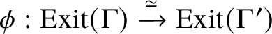
extends to a natural equivalence

between the incidence diagrams.
Definition 7.8. An equivalence between two ribbon graphs with spin structure $\left (\Gamma ,\tilde {I}^{2}_{\Gamma }\right ),\left (\Gamma ^{\prime },{\tilde {I}^{2}}_{\Gamma ^{\prime }}\right )$
consists of an equivalence
$\left (\Gamma ,\tilde {I}^{2}_{\Gamma }\right ),\left (\Gamma ^{\prime },{\tilde {I}^{2}}_{\Gamma ^{\prime }}\right )$
consists of an equivalence

of ribbon graphs together with a lift

of

The main result of this section is the following:
Proposition 7.9. Let $\mathbf {S}$
be an oriented marked surface equipped with an ideal triangulation
$\mathbf {S}$
be an oriented marked surface equipped with an ideal triangulation $\mathcal {T}$
and let
$\mathcal {T}$
and let $\Sigma =\mathbf {S}\backslash (M\cap \mathbf {S}^{\circ })$
be the surface without the interior marked points.
$\Sigma =\mathbf {S}\backslash (M\cap \mathbf {S}^{\circ })$
be the surface without the interior marked points.
-
1. For every spin structure U on
$\Sigma $
, there exists a
$\Gamma _{\mathcal {T}}$
-parametrised perverse schober
$\mathcal {F}_{\mathcal {T}}^{U}$
. If two spin structures
$U,U^{\prime }$
on
$\Sigma $
are equivalent, then there exists an equivalence of parametrised perverse schobers (74)If
$$ \begin{align} \mathcal{F}_{\mathcal{T}}^{U}\simeq \mathcal{F}_{\mathcal{T}}^{U^{\prime}}. \end{align} $$
$\operatorname {char}(k)\neq 2$
, the converse is also true – that is, if there exists an equivalence as in formula (74), then
$U\simeq U^{\prime }$
.
-
2. Given a parametrised perverse schober
$\mathcal {F}_{\mathcal {T}}$
as constructed in the proof of Theorem 6.1, there exist a spin structure U on
$\Sigma $
and an equivalence of parametrised perverse schobers
$$ \begin{align*} \mathcal{F}_{\mathcal{T}}\simeq \mathcal{F}^{U}_{\mathcal{T}}. \end{align*} $$


Definition 7.10. A ribbon graph $\Gamma $
is called trivalent if all vertices have valency
$\Gamma $
is called trivalent if all vertices have valency $3$
.
$3$
.
Definition 7.11. We denote by $M_{2}$
the subcategory of
$M_{2}$
the subcategory of $\Lambda _{2}$
spanned by the two objects
$\Lambda _{2}$
spanned by the two objects $[1],[2]$
and morphisms generated under composition by
$[1],[2]$
and morphisms generated under composition by $\tau ^{1}:[1]\rightarrow [1]$
,
$\tau ^{1}:[1]\rightarrow [1]$
, $\tau ^{2}:[2]\rightarrow [2]$
and
$\tau ^{2}:[2]\rightarrow [2]$
and $\delta ^{l}:[1] \rightarrow [2]$
for
$\delta ^{l}:[1] \rightarrow [2]$
for $l=1,2,3$
.
$l=1,2,3$
.
Remark 7.12. Let $\Gamma $
be a trivalent ribbon graph and
$\Gamma $
be a trivalent ribbon graph and $\tilde {I}^{2}:\operatorname {Exit}(\Gamma )\rightarrow \Lambda _{2}$
a spin structure. Then
$\tilde {I}^{2}:\operatorname {Exit}(\Gamma )\rightarrow \Lambda _{2}$
a spin structure. Then $\tilde {I}^{2}$
factors through the inclusion
$\tilde {I}^{2}$
factors through the inclusion $M_{2}\rightarrow \Lambda _{2}$
.
$M_{2}\rightarrow \Lambda _{2}$
.
Proof of Proposition 7.9.
Consider the morphism of dg-algebras

, the pullback functor $\varphi ^{*}:\operatorname {dgMod}(k[t_{1}])\rightarrow \operatorname {dgMod}(k[t_{1}])$
and Notation 5.11. We further denote by
$\varphi ^{*}:\operatorname {dgMod}(k[t_{1}])\rightarrow \operatorname {dgMod}(k[t_{1}])$
and Notation 5.11. We further denote by $T_{D_{3}}:D_{3}\rightarrow D_{3}$
the dg-functor determined by
$T_{D_{3}}:D_{3}\rightarrow D_{3}$
the dg-functor determined by
 $$ \begin{align*} x,y,z&\mapsto y,z,x,\\ a,b,c&\mapsto b,c,a,\\ a^{*},b^{*},c^{*}&\mapsto -b^{*},-c^{*},-a^{*}. \end{align*} $$
We define a functor
 $$ \begin{align*} \mathcal{Q}:M_{2}^{\operatorname{op}}\rightarrow \operatorname{dgCat}_{k} \end{align*} $$
by
 $$ \begin{align*} \mathcal{Q}([2])&=D_{3}, \\ \mathcal{Q}([1])&=k[t_{1}], \\ \mathcal{Q}\left(\tau^{2}\right)&=T_{D_{3}}, \\ \mathcal{Q}\left(\tau^{1}\right)&=\varphi^{*}, \\ \mathcal{Q}(\delta_{1})&=i_{1}^{+}, \\ \mathcal{Q}(\delta_{2})&=i_{2}^{-}, \\ \mathcal{Q}(\delta_{3})&=i_{3}^{+}. \end{align*} $$
Let $\mathcal {T}$
be an ideal triangulation and
$\mathcal {T}$
be an ideal triangulation and $\Gamma _{\mathcal {T}}$
the dual ribbon graph. Given a spin structure U on
$\Gamma _{\mathcal {T}}$
the dual ribbon graph. Given a spin structure U on $\Gamma _{\mathcal {T}}$
described in terms of
$\Gamma _{\mathcal {T}}$
described in terms of $\tilde {I}^{2}:\operatorname {Exit}(\Gamma _{\mathcal {T}})\rightarrow M_{2}$
, we obtain a parametrised perverse schober
$\tilde {I}^{2}:\operatorname {Exit}(\Gamma _{\mathcal {T}})\rightarrow M_{2}$
, we obtain a parametrised perverse schober $\mathcal {F}_{\mathcal {T}}^{U}$
defined via its left dual
$\mathcal {F}_{\mathcal {T}}^{U}$
defined via its left dual

Given an equivalence of spin structures $U\simeq U^{\prime }$
, expressed in terms of an equivalence of ribbon graphs with spin structure
$U\simeq U^{\prime }$
, expressed in terms of an equivalence of ribbon graphs with spin structure $\left (\Gamma _{\mathcal {T}},\tilde {I}^{2}\right )\simeq \left (\Gamma _{\mathcal {T}},\left (\tilde {I}^{2}\right )^{\prime }\right )$
, it is immediate from the construction that there is an equivalence between
$\left (\Gamma _{\mathcal {T}},\tilde {I}^{2}\right )\simeq \left (\Gamma _{\mathcal {T}},\left (\tilde {I}^{2}\right )^{\prime }\right )$
, it is immediate from the construction that there is an equivalence between $\mathcal {F}^{U}_{\mathcal {T}}$
and
$\mathcal {F}^{U}_{\mathcal {T}}$
and $\mathcal {F}^{U^{\prime }}_{\mathcal {T}}$
. For the converse, we note that by a standard result, spin structures on
$\mathcal {F}^{U^{\prime }}_{\mathcal {T}}$
. For the converse, we note that by a standard result, spin structures on $\Sigma $
are classified by
$\Sigma $
are classified by $\operatorname {H}^{1}(\Sigma ,\mathbb {Z}_{2})$
. Thus, if two spin structures differ, then there exists an embedded circle in
$\operatorname {H}^{1}(\Sigma ,\mathbb {Z}_{2})$
. Thus, if two spin structures differ, then there exists an embedded circle in $\Gamma _{\mathcal {T}}$
such that the restrictions of the spin structures to the full ribbon subgraph spanned by the vertices on the circle differ. Up to equivalence of spin structures, these two spin structures can be assumed to be identical, except that they assign to the incidence of some fixed edge lying on the circle and some fixed vertex two morphisms
$\Gamma _{\mathcal {T}}$
such that the restrictions of the spin structures to the full ribbon subgraph spanned by the vertices on the circle differ. Up to equivalence of spin structures, these two spin structures can be assumed to be identical, except that they assign to the incidence of some fixed edge lying on the circle and some fixed vertex two morphisms $[1]\rightarrow [2]$
in
$[1]\rightarrow [2]$
in $\Lambda _{2}$
which differ exactly by precomposition with
$\Lambda _{2}$
which differ exactly by precomposition with $\tau ^{1}$
. The corresponding restrictions of the parametrised perverse schobers thus differ at this subgraph in terms of their monodromy by
$\tau ^{1}$
. The corresponding restrictions of the parametrised perverse schobers thus differ at this subgraph in terms of their monodromy by $\mathcal {D}(\phi ^{*})$
. Note that the assumption
$\mathcal {D}(\phi ^{*})$
. Note that the assumption $\operatorname {char}(k)\neq 2$
implies
$\operatorname {char}(k)\neq 2$
implies $\mathcal {D}(\phi ^{*})\neq \operatorname {id}_{\mathcal {D}\left (k\left [t_{1}\right ]\right )}$
. The two parametrised perverse schobers can thus not be equivalent, showing the converse implication.
$\mathcal {D}(\phi ^{*})\neq \operatorname {id}_{\mathcal {D}\left (k\left [t_{1}\right ]\right )}$
. The two parametrised perverse schobers can thus not be equivalent, showing the converse implication.
Let $\mathcal {T}$
be an ideal triangulation and consider a parametrised perverse schober
$\mathcal {T}$
be an ideal triangulation and consider a parametrised perverse schober $\mathcal {F}_{\mathcal {T}}$
as constructed in Theorem 6.1. In the following we describe a spin structure U on
$\mathcal {F}_{\mathcal {T}}$
as constructed in Theorem 6.1. In the following we describe a spin structure U on $\Gamma _{\mathcal {T}}$
such that
$\Gamma _{\mathcal {T}}$
such that $\mathcal {F}_{\mathcal {T}}^{U}\simeq \mathcal {F}_{\mathcal {T}}$
. We follow the iterative procedure and notation used in the proof of Theorem 6.1. Starting with any ideal triangle
$\mathcal {F}_{\mathcal {T}}^{U}\simeq \mathcal {F}_{\mathcal {T}}$
. We follow the iterative procedure and notation used in the proof of Theorem 6.1. Starting with any ideal triangle $\mathcal {T}_{1}$
of
$\mathcal {T}_{1}$
of $\mathcal {T}$
, one can directly find a spin structure U on
$\mathcal {T}$
, one can directly find a spin structure U on $\Gamma _{\mathcal {T}_{1}}$
such that
$\Gamma _{\mathcal {T}_{1}}$
such that $\mathcal {F}_{\mathcal {T}_{1}}\simeq \mathcal {F}_{\mathcal {T}_{1}}^{U}$
. We continue by extending the spin structure in each induction step by gluing. Consider an ideal triangulation
$\mathcal {F}_{\mathcal {T}_{1}}\simeq \mathcal {F}_{\mathcal {T}_{1}}^{U}$
. We continue by extending the spin structure in each induction step by gluing. Consider an ideal triangulation $\mathcal {T}_{n+1}$
, obtained from gluing two ideal triangulations
$\mathcal {T}_{n+1}$
, obtained from gluing two ideal triangulations $\mathcal {T}_{n}$
and
$\mathcal {T}_{n}$
and $\mathcal {T}_{1}$
equipped with spin structures. There is a spin structure
$\mathcal {T}_{1}$
equipped with spin structures. There is a spin structure $\tilde {I}_{n+1}^{2}:\operatorname {Exit}\left (\Gamma _{\mathcal {T}_{n+1}}\right )\rightarrow M_{2}$
on
$\tilde {I}_{n+1}^{2}:\operatorname {Exit}\left (\Gamma _{\mathcal {T}_{n+1}}\right )\rightarrow M_{2}$
on $\Gamma _{\mathcal {T}_{n+1}}$
with the property that the restriction to
$\Gamma _{\mathcal {T}_{n+1}}$
with the property that the restriction to $\operatorname {Exit}\left (\Gamma _{\mathcal {T}_{n}}\right )$
and
$\operatorname {Exit}\left (\Gamma _{\mathcal {T}_{n}}\right )$
and $\operatorname {Exit}\left (\Gamma _{\mathcal {T}_{1}}\right )$
recovers the respective spin structures of
$\operatorname {Exit}\left (\Gamma _{\mathcal {T}_{1}}\right )$
recovers the respective spin structures of $\Gamma _{\mathcal {T}_{n}}$
and
$\Gamma _{\mathcal {T}_{n}}$
and $\Gamma _{\mathcal {T}_{1}}$
. We now modify
$\Gamma _{\mathcal {T}_{1}}$
. We now modify $\tilde {I}_{n+1}^{2}$
to obtain the desired spin structure U on
$\tilde {I}_{n+1}^{2}$
to obtain the desired spin structure U on $\Gamma _{\mathcal {T}_{n+1}}$
. At each edge e used in the gluing of
$\Gamma _{\mathcal {T}_{n+1}}$
. At each edge e used in the gluing of $\mathcal {T}_{n}$
and
$\mathcal {T}_{n}$
and $\mathcal {T}_{1}$
and connecting two vertices
$\mathcal {T}_{1}$
and connecting two vertices $v_{n}$
and
$v_{n}$
and $v_{1}$
in
$v_{1}$
in $\Gamma _{\mathcal {T}_{n}}$
and
$\Gamma _{\mathcal {T}_{n}}$
and $\Gamma _{\mathcal {T}_{1}}$
, respectively, the spin structure
$\Gamma _{\mathcal {T}_{1}}$
, respectively, the spin structure $\tilde {I}^{2}_{n+1}$
is locally of the form
$\tilde {I}^{2}_{n+1}$
is locally of the form

We obtain U by changing the spin structure $I^{2}_{n+1}$
at each edge e used in the gluing of
$I^{2}_{n+1}$
at each edge e used in the gluing of $\Gamma _{\mathcal {T}_{n}}$
and
$\Gamma _{\mathcal {T}_{n}}$
and $\Gamma _{\mathcal {T}_{1}}$
in the local picture to
$\Gamma _{\mathcal {T}_{1}}$
in the local picture to

if the superscripts of the associated functors $i_{e}^{1}=i_{e}^{\pm }$
and
$i_{e}^{1}=i_{e}^{\pm }$
and $i_{e}^{n}=i_{e}^{\pm }$
, appearing in the proof of Theorem 6.1, match. The resulting parametrised perverse schober
$i_{e}^{n}=i_{e}^{\pm }$
, appearing in the proof of Theorem 6.1, match. The resulting parametrised perverse schober $\mathcal {F}_{\mathcal {T}_{n+1}}^{U}$
is then equivalent to
$\mathcal {F}_{\mathcal {T}_{n+1}}^{U}$
is then equivalent to $\mathcal {F}_{\mathcal {T}_{n+1}}$
. This shows statement
$\mathcal {F}_{\mathcal {T}_{n+1}}$
. This shows statement $2$
, thus completing the proof.
$2$
, thus completing the proof.
7.2 Coefficients in spectra
Let $\mathcal {T}$
be an ideal triangulation of an oriented marked surface and consider the construction of the parametrised perverse schober
$\mathcal {T}$
be an ideal triangulation of an oriented marked surface and consider the construction of the parametrised perverse schober $\mathcal {F}_{\mathcal {T}}$
of Theorem 6.1. Given any stable
$\mathcal {F}_{\mathcal {T}}$
of Theorem 6.1. Given any stable $\infty $
-category
$\infty $
-category $\mathcal {D}$
, we can construct a parametrised perverse schober
$\mathcal {D}$
, we can construct a parametrised perverse schober $\mathcal {F}_{\mathcal {T}}(\mathcal {D})$
by replacing the spherical adjunction at each vertex with the spherical adjunction
$\mathcal {F}_{\mathcal {T}}(\mathcal {D})$
by replacing the spherical adjunction at each vertex with the spherical adjunction
 $$ \begin{align*} f^{*}:\mathcal{D}\longleftrightarrow \operatorname{Fun}\left(S^{2},\mathcal{D}\right):f_{*}\\[-15pt] \end{align*} $$
and the autoequivalence $T=T_{\operatorname {Fun}\left (S^{2},\mathcal {D}(k)\right )}[2]$
(used there for fixing the correct signs) by the
$T=T_{\operatorname {Fun}\left (S^{2},\mathcal {D}(k)\right )}[2]$
(used there for fixing the correct signs) by the $2$
-fold suspension of the cotwist functor
$2$
-fold suspension of the cotwist functor $T_{\operatorname {Fun}\left (S^{2},\mathcal {D}\right )}[2]$
of the same adjunction
$T_{\operatorname {Fun}\left (S^{2},\mathcal {D}\right )}[2]$
of the same adjunction $f^{*}\dashv f_{*}$
but with values in
$f^{*}\dashv f_{*}$
but with values in $\mathcal {D}$
instead of
$\mathcal {D}$
instead of $\mathcal {D}(k)$
. The goal of this section is to discuss which results of this paper translate to this more general setting.
$\mathcal {D}(k)$
. The goal of this section is to discuss which results of this paper translate to this more general setting.
We begin by noting that the main result which works irrespective of the choice of $\mathcal {D}$
is the construction of the derived equivalence
$\mathcal {D}$
is the construction of the derived equivalence
 $$ \begin{align*} \mu_{e}:\mathcal{H}(\Gamma_{\mathcal{T}},\mathcal{F}_{\mathcal{T}}(\mathcal{D}))\simeq \mathcal{H}\left(\Gamma_{\mathcal{T}^{\;\prime}},\mathcal{F}_{\mathcal{T}^{\;\prime}}(\mathcal{D})\right)\\[-15pt] \end{align*} $$
of Section 6.4 associated to the flip of the edge e of the triangulation $\mathcal {T}$
.
$\mathcal {T}$
.
More results extend in the case where $\mathcal {D}=\operatorname {RMod}_{R}$
is the
$\mathcal {D}=\operatorname {RMod}_{R}$
is the $\infty $
-category of right modules of an
$\infty $
-category of right modules of an $\mathbb {E}_{\infty }$
-ring spectrum R. We can, for example, choose R to be the sphere spectrum, so that
$\mathbb {E}_{\infty }$
-ring spectrum R. We can, for example, choose R to be the sphere spectrum, so that $\mathcal {D}\simeq \operatorname {Sp}$
is the
$\mathcal {D}\simeq \operatorname {Sp}$
is the $\infty $
-category of spectra. The construction of the spherical/exceptional objects
$\infty $
-category of spectra. The construction of the spherical/exceptional objects $S_{e}$
, the objects
$S_{e}$
, the objects $C_{p}$
and the projective objects
$C_{p}$
and the projective objects $P_{e}$
given in Section 6.3 works in the same way for
$P_{e}$
given in Section 6.3 works in the same way for $\mathcal {H}(\Gamma _{\mathcal {T}},\mathcal {F}_{\mathcal {T}}(\operatorname {RMod}_{R}))$
. We denote by
$\mathcal {H}(\Gamma _{\mathcal {T}},\mathcal {F}_{\mathcal {T}}(\operatorname {RMod}_{R}))$
. We denote by $R[t_{n}]$
the free algebra object in
$R[t_{n}]$
the free algebra object in $\operatorname {RMod}_{R}$
generated by
$\operatorname {RMod}_{R}$
generated by $R[n]$
. Note that if
$R[n]$
. Note that if $R=k$
is a commutative ring, there exists an equivalence
$R=k$
is a commutative ring, there exists an equivalence $R[t_{n}]\simeq k[t_{n}]$
. We show in Proposition 7.15 that there exists an equivalence of
$R[t_{n}]\simeq k[t_{n}]$
. We show in Proposition 7.15 that there exists an equivalence of $\infty $
-categories
$\infty $
-categories $\operatorname {Fun}(S^{n},\operatorname {RMod}_{R})\simeq \operatorname {RMod}_{R\left [t_{n-1}\right ]}$
. We thus find a compact generator of the
$\operatorname {Fun}(S^{n},\operatorname {RMod}_{R})\simeq \operatorname {RMod}_{R\left [t_{n-1}\right ]}$
. We thus find a compact generator of the $\infty $
-category
$\infty $
-category $\mathcal {H}(\Gamma _{\mathcal {T}},\mathcal {F}_{\mathcal {T}}(\operatorname {RMod}_{R}))$
, as in Proposition 6.7, given by the sum of the images of
$\mathcal {H}(\Gamma _{\mathcal {T}},\mathcal {F}_{\mathcal {T}}(\operatorname {RMod}_{R}))$
, as in Proposition 6.7, given by the sum of the images of $R[t_{1}]\in \operatorname {RMod}_{R\left [t_{1}\right ]}\simeq \operatorname {Fun}\left (S^{2},\operatorname {RMod}_{R}\right )$
under the left adjoints of the evaluation functors to the edges of
$R[t_{1}]\in \operatorname {RMod}_{R\left [t_{1}\right ]}\simeq \operatorname {Fun}\left (S^{2},\operatorname {RMod}_{R}\right )$
under the left adjoints of the evaluation functors to the edges of $\Gamma _{\mathcal {T}}$
. Furthermore, Proposition 6.9, describing the images of the
$\Gamma _{\mathcal {T}}$
. Furthermore, Proposition 6.9, describing the images of the $P_{e}$
under the derived equivalences, also translates. Contrary to the dg-setting, however, it is not clear whether the endomorphism algebra of the compact generator admits an explicit description.
$P_{e}$
under the derived equivalences, also translates. Contrary to the dg-setting, however, it is not clear whether the endomorphism algebra of the compact generator admits an explicit description.
Crucial for a relation between the construction of $\mathcal {F}_{\mathcal {T}}(\mathcal {D}(k))$
and spin structures on the surface without the interior marked points
$\mathcal {F}_{\mathcal {T}}(\mathcal {D}(k))$
and spin structures on the surface without the interior marked points $\Sigma $
in Section 7.1 is the observation that the suspended cotwist functor
$\Sigma $
in Section 7.1 is the observation that the suspended cotwist functor $T_{\operatorname {Fun}\left (S^{2},\mathcal {D}(k)\right )}[2]$
is an involution – that is,
$T_{\operatorname {Fun}\left (S^{2},\mathcal {D}(k)\right )}[2]$
is an involution – that is,
 $$ \begin{align*} \left( T_{\operatorname{Fun}\left(S^{2},\mathcal{D}(k)\right)}[2]\right)^{2}\simeq {\rm id}_{\operatorname{Fun}\left(S^{2},\mathcal{D}(k)\right)}. \end{align*} $$
It seems likely that if the cotwist functor $T_{\operatorname {Fun}\left (S^{2},\mathcal {D}\right )}[2]$
is also an involution, Proposition 7.9 can be generalised to
$T_{\operatorname {Fun}\left (S^{2},\mathcal {D}\right )}[2]$
is also an involution, Proposition 7.9 can be generalised to $\mathcal {F}_{\mathcal {T}}(\mathcal {D})$
. The remainder of this section consists of a proof of Proposition 7.15 and a conjecture for a description of
$\mathcal {F}_{\mathcal {T}}(\mathcal {D})$
. The remainder of this section consists of a proof of Proposition 7.15 and a conjecture for a description of $T_{\operatorname {Fun}\left (S^{2},\mathcal {D}\right )}$
and an algebraic description of
$T_{\operatorname {Fun}\left (S^{2},\mathcal {D}\right )}$
and an algebraic description of $T_{\operatorname {Fun}\left (S^{2},\operatorname {RMod}_{R}\right )}$
.
$T_{\operatorname {Fun}\left (S^{2},\operatorname {RMod}_{R}\right )}$
.
The following lemma is a generalisation of Lemma 5.3:
Lemma 7.13. Consider the morphism of simplicial sets $g:L\rightarrow \ast $
and the associated pullback functor
$g:L\rightarrow \ast $
and the associated pullback functor $g^{*}:\operatorname {RMod}_{R}\rightarrow \operatorname {Fun}(L,\operatorname {RMod}_{R})$
. There exists an equivalence of R-linear
$g^{*}:\operatorname {RMod}_{R}\rightarrow \operatorname {Fun}(L,\operatorname {RMod}_{R})$
. There exists an equivalence of R-linear $\infty $
-categories
$\infty $
-categories
 $$ \begin{align*} \operatorname{Fun}(L,\operatorname{RMod}_{R})\simeq \operatorname{RMod}_{R\left[t_{0}\right]} \end{align*} $$
such that the following diagram commutes:

Here $\phi ^{*}$
denotes the pullback functor along the morphism of R-algebras
$\phi ^{*}$
denotes the pullback functor along the morphism of R-algebras $R[t_{0}]\rightarrow R$
, determined on the generator by the morphism
$R[t_{0}]\rightarrow R$
, determined on the generator by the morphism
![]() in
in $\operatorname {RMod}_{R}$
.
$\operatorname {RMod}_{R}$
.
Proof. Consider the object $X\in \operatorname {Fun}(L,\operatorname {RMod}_{R})$
given by the diagram
$X\in \operatorname {Fun}(L,\operatorname {RMod}_{R})$
given by the diagram
 in
in $\operatorname {RMod}_{R}$
. Let
$\operatorname {RMod}_{R}$
. Let $h:\ast \rightarrow L$
be the morphism of simplicial sets given by inclusion of the unique vertex and consider the associated pullback functor
$h:\ast \rightarrow L$
be the morphism of simplicial sets given by inclusion of the unique vertex and consider the associated pullback functor $h^{*}:\operatorname {RMod}_{R}\rightarrow \operatorname {Fun}(L,\operatorname {RMod}_{R})$
with right adjoint
$h^{*}:\operatorname {RMod}_{R}\rightarrow \operatorname {Fun}(L,\operatorname {RMod}_{R})$
with right adjoint $h_{*}$
given by evaluation at
$h_{*}$
given by evaluation at $\ast \in L$
. We prove that
$\ast \in L$
. We prove that $X\simeq h^{*}(R)$
by showing that
$X\simeq h^{*}(R)$
by showing that
![]() , where
, where
![]() is the R-linear morphism object functor of [Reference LurieLur17, 4.2.1.28].
is the R-linear morphism object functor of [Reference LurieLur17, 4.2.1.28].
Set $Y\in \operatorname {Fun}(L,\operatorname {RMod}_{R})$
. The morphism object
$Y\in \operatorname {Fun}(L,\operatorname {RMod}_{R})$
. The morphism object $\operatorname {Mor}_{\operatorname {Fun}\left (L,\operatorname {RMod}_{R}\right )}(X,Y)$
is equivalent to the equaliser
$\operatorname {Mor}_{\operatorname {Fun}\left (L,\operatorname {RMod}_{R}\right )}(X,Y)$
is equivalent to the equaliser

where l is the unique nondegenerate $1$
-simplex of L. This can be seen as follows. Consider the simplicial set
$1$
-simplex of L. This can be seen as follows. Consider the simplicial set $L^{\prime }$
consisting of four vertices
$L^{\prime }$
consisting of four vertices $x_{1},x_{2},x_{3},x_{4}$
and four nondegenerate
$x_{1},x_{2},x_{3},x_{4}$
and four nondegenerate $1$
-simplices
$1$
-simplices $l_{1},l_{2},l_{3},l_{4}$
arranged as follows:
$l_{1},l_{2},l_{3},l_{4}$
arranged as follows:

The morphism of simplicial sets $p:L^{\prime }\rightarrow L$
, mapping all vertices to
$p:L^{\prime }\rightarrow L$
, mapping all vertices to $\ast \in L$
,
$\ast \in L$
, $l_{1}$
to l and
$l_{1}$
to l and $l_{2},l_{3},l_{4}$
to the degenerate
$l_{2},l_{3},l_{4}$
to the degenerate $1$
-simplex, induces a fully faithful R-linear functor
$1$
-simplex, induces a fully faithful R-linear functor $p^{*}:\operatorname {Fun}(L,\operatorname {RMod}_{R})\rightarrow \operatorname {Fun}(L^{\prime },\operatorname {RMod}_{R})$
. The description of
$p^{*}:\operatorname {Fun}(L,\operatorname {RMod}_{R})\rightarrow \operatorname {Fun}(L^{\prime },\operatorname {RMod}_{R})$
. The description of $\operatorname {Mor}_{\operatorname {Fun}\left (L,\operatorname {RMod}_{R}\right )}(X,Y)\simeq \operatorname {Mor}_{\operatorname {Fun}\left (L^{\prime },\operatorname {RMod}_{R}\right )}(p^{*}(X),p^{*}(Y))$
as an equaliser can now be obtained by using a pushout description of
$\operatorname {Mor}_{\operatorname {Fun}\left (L,\operatorname {RMod}_{R}\right )}(X,Y)\simeq \operatorname {Mor}_{\operatorname {Fun}\left (L^{\prime },\operatorname {RMod}_{R}\right )}(p^{*}(X),p^{*}(Y))$
as an equaliser can now be obtained by using a pushout description of $p^{*}(X)\simeq X_{1}\amalg _{X_{3}}X_{2}$
, with
$p^{*}(X)\simeq X_{1}\amalg _{X_{3}}X_{2}$
, with

and the fact that
is an exact functor. The equaliser is given by $h_{*}(Y)$
, and the morphism of R-modules
$h_{*}(Y)$
, and the morphism of R-modules $h_{*}(Y)\rightarrow \prod _{i\in \mathbb {N}} h_{*}(Y)$
is informally given by mapping
$h_{*}(Y)\rightarrow \prod _{i\in \mathbb {N}} h_{*}(Y)$
is informally given by mapping $z\in h_{*}(Y)$
to
$z\in h_{*}(Y)$
to $\left (Y(l)^{i}(z)\right )_{i\in \mathbb {N}}\in \prod _{i\in \mathbb {N}} h_{*}(Y)$
. We note that the equivalence
$\left (Y(l)^{i}(z)\right )_{i\in \mathbb {N}}\in \prod _{i\in \mathbb {N}} h_{*}(Y)$
. We note that the equivalence $\operatorname {Mor}_{\operatorname {Fun}\left (L,\operatorname {RMod}_{R}\right )}(X,Y)\simeq h_{*}(Y)$
is functorial in Y, so that indeed
$\operatorname {Mor}_{\operatorname {Fun}\left (L,\operatorname {RMod}_{R}\right )}(X,Y)\simeq h_{*}(Y)$
is functorial in Y, so that indeed
.
It follows that X is a compact generator of $\operatorname {Fun}(L,\operatorname {RMod}_{R})$
. Applying [Reference LurieLur17, Proposition 4.1.1.18], we further obtain an equivalence of R-linear ring spectra
$\operatorname {Fun}(L,\operatorname {RMod}_{R})$
. Applying [Reference LurieLur17, Proposition 4.1.1.18], we further obtain an equivalence of R-linear ring spectra $\operatorname {End}_{R}(X)\simeq R[t_{0}]$
, showing the existence of an equivalence of R-linear
$\operatorname {End}_{R}(X)\simeq R[t_{0}]$
, showing the existence of an equivalence of R-linear $\infty $
-categories
$\infty $
-categories $\operatorname {Fun}(L,\operatorname {RMod}_{R})\simeq \operatorname {RMod}_{R\left [t_{0}\right ]}$
.
$\operatorname {Fun}(L,\operatorname {RMod}_{R})\simeq \operatorname {RMod}_{R\left [t_{0}\right ]}$
.
The commutativity of diagram (75) can be checked using the fact that the R-linear functors $\phi ^{*},g^{*}:\operatorname {RMod}_{R}\rightarrow \operatorname {RMod}_{R\left [t_{0}\right ]}$
are fully determined by, respectively,
$\phi ^{*},g^{*}:\operatorname {RMod}_{R}\rightarrow \operatorname {RMod}_{R\left [t_{0}\right ]}$
are fully determined by, respectively, $\phi ^{*}(R)$
and
$\phi ^{*}(R)$
and $g^{*}(R)$
[Reference LurieLur17, Section 4.8.4].
$g^{*}(R)$
[Reference LurieLur17, Section 4.8.4].
Lemma 7.14.
-
1. There exists a pushout diagram in
$\operatorname {LinCat}_{R}$
as follows: (76) -
2. Set
$n\geq 2$
. There exists a pushout diagram in
$\operatorname {LinCat}_{R}$
as follows: (77)


Proof. The proof of Lemma 5.4 directly generalises.
We now prove the analogue of Proposition 5.5.
Proposition 7.15. Set $n\geq 2$
. There exists an equivalence of R-linear
$n\geq 2$
. There exists an equivalence of R-linear $\infty $
-categories
$\infty $
-categories
 $$ \begin{align} \operatorname{Fun}(S^{n},\operatorname{RMod}_{R})\simeq \operatorname{RMod}_{R\left[t_{n-1}\right]}, \end{align} $$
such that the following diagram in $\operatorname {LinCat}_{R}$
commutes:
$\operatorname {LinCat}_{R}$
commutes:

Here G denotes the monadic functor and $\phi ^{*}$
the pullback functor along the morphism of R-algebras
$\phi ^{*}$
the pullback functor along the morphism of R-algebras $\phi :R[t_{n-1}]\rightarrow R$
determined on the generator by the morphism
$\phi :R[t_{n-1}]\rightarrow R$
determined on the generator by the morphism
 in
in $\operatorname {RMod}_{R}$
.
$\operatorname {RMod}_{R}$
.
Proof. Consider the following bi-Cartesian square in $\operatorname {RMod}_{R}$
:
$\operatorname {RMod}_{R}$
:

Applying the colimit-preserving free R-algebra functor $\operatorname {RMod}_{R}\rightarrow \operatorname {Alg}(\operatorname {RMod}_{R})$
yields the following pushout diagram of R-algebras:
$\operatorname {RMod}_{R}\rightarrow \operatorname {Alg}(\operatorname {RMod}_{R})$
yields the following pushout diagram of R-algebras:

Consider the morphism of ring spectra
, determined from the universal property by the morphism
in $\operatorname {RMod}_{R}$
. Using the commutativity of the diagram
$\operatorname {RMod}_{R}$
. Using the commutativity of the diagram

it follows that for $n=1$
the image of diagram (80) under
$n=1$
the image of diagram (80) under $\theta :\operatorname {Alg}(\operatorname {RMod})\rightarrow \operatorname {LinCat}_{R}$
is equivalent to the pushout diagram (76). It follows that there exists an equivalence of R-linear
$\theta :\operatorname {Alg}(\operatorname {RMod})\rightarrow \operatorname {LinCat}_{R}$
is equivalent to the pushout diagram (76). It follows that there exists an equivalence of R-linear $\infty $
-categories
$\infty $
-categories $\operatorname {Fun}\left (S^{2},\operatorname {RMod}_{R}\right )\simeq \operatorname {RMod}_{R\left [t_{1}\right ]}$
. Using the fact that the monadic functor G is equivalent to the pullback along
$\operatorname {Fun}\left (S^{2},\operatorname {RMod}_{R}\right )\simeq \operatorname {RMod}_{R\left [t_{1}\right ]}$
. Using the fact that the monadic functor G is equivalent to the pullback along $R\rightarrow R[t_{1}]$
, we find that the upper half of diagram (38) commutes.
$R\rightarrow R[t_{1}]$
, we find that the upper half of diagram (38) commutes.
Using the fact that $f_!\circ i_!\simeq \operatorname {id}_{\operatorname {RMod}_{R}}$
(see Remark 5.6), we obtain the following commutative diagram:
$f_!\circ i_!\simeq \operatorname {id}_{\operatorname {RMod}_{R}}$
(see Remark 5.6), we obtain the following commutative diagram:

Diagram (81) is equivalent to the image under $\theta $
of the following diagram in
$\theta $
of the following diagram in $\operatorname {Alg}(\operatorname {RMod}_{R})$
:
$\operatorname {Alg}(\operatorname {RMod}_{R})$
:

By the universal property of the pushout in $\operatorname {Alg}(\operatorname {RMod}_{R})$
, there exists a unique morphism of ring spectra
$\operatorname {Alg}(\operatorname {RMod}_{R})$
, there exists a unique morphism of ring spectra $R[t_{1}]\rightarrow R$
such that diagram (82) commutes. Such a map is given by
$R[t_{1}]\rightarrow R$
such that diagram (82) commutes. Such a map is given by $\phi $
. It follows that the functor
$\phi $
. It follows that the functor $f_!$
is equivalent to
$f_!$
is equivalent to $\theta (\phi )$
and, using [Reference LurieLur17, 4.6.2.17] also, that the functor
$\theta (\phi )$
and, using [Reference LurieLur17, 4.6.2.17] also, that the functor $f^{*}$
is equivalent to the pullback functor along
$f^{*}$
is equivalent to the pullback functor along $\phi $
.
$\phi $
.
For $n\geq 2$
, we can continue by induction and as before. The image of diagram (80) under the functor
$n\geq 2$
, we can continue by induction and as before. The image of diagram (80) under the functor $\theta $
is the pushout diagram (77). We thus find the desired equivalence
$\theta $
is the pushout diagram (77). We thus find the desired equivalence $\operatorname {Fun}(S^{n},\operatorname {RMod}_{R})\simeq \operatorname {RMod}_{R\left [t_{n-1}\right ]}$
, so the upper half of diagram (79) commutes. Analogous to the case
$\operatorname {Fun}(S^{n},\operatorname {RMod}_{R})\simeq \operatorname {RMod}_{R\left [t_{n-1}\right ]}$
, so the upper half of diagram (79) commutes. Analogous to the case $n=1$
, it can be checked that the lower half of diagram (79) commutes.
$n=1$
, it can be checked that the lower half of diagram (79) commutes.
Our proof of Proposition 5.7 characterising the cotwist functor of the spherical adjunction $f^{*}\dashv f_{*}$
does not directly generalise to the spectral setting. We conjecture the following:
$f^{*}\dashv f_{*}$
does not directly generalise to the spectral setting. We conjecture the following:
Conjecture 7.16. For any stable $\infty $
-category
$\infty $
-category $\mathcal {D}$
and
$\mathcal {D}$
and $n\geq 2$
, consider the cotwist functor
$n\geq 2$
, consider the cotwist functor $T_{\operatorname {Fun}\left (S^{n},\mathcal {D}\right )}$
of the spherical adjunction
$T_{\operatorname {Fun}\left (S^{n},\mathcal {D}\right )}$
of the spherical adjunction $f^{*}:\mathcal {D}\leftrightarrow \operatorname {Fun}(S^{n},\mathcal {D}):f_{*}$
(see Proposition 5.1).
$f^{*}:\mathcal {D}\leftrightarrow \operatorname {Fun}(S^{n},\mathcal {D}):f_{*}$
(see Proposition 5.1).
-
1. Let R be an
$\mathbb {E}_{\infty }$
-ring spectrum and
$\mathcal {D}=\operatorname {RMod}_{R}$
. Let
$\varphi :R[t_{n-1}]\rightarrow R[t_{n-1}]$
be the equivalence of ring spectra determined by
$\varphi (t_{n-1})=(-1)^{n-1}t_{n-1}$
(via the involved universal properties). There exists a commutative diagram in
$\operatorname {LinCat}_{R}$
as follows: -
2. Denote by
$S^{n}_{\operatorname {top}}$
the topological n-sphere embedded as the unit sphere into
$\mathbb {R}^{n+1}$
, so that its singular set is given by
$\operatorname {Sing}\left (S^{n}_{\operatorname {top}}\right )=S^{n}$
. Let
$r:S^{n}_{\operatorname {top}}\rightarrow S^{n}_{\operatorname {top}}$
be the antipodal map, mapping
$x\in S^{n}_{\operatorname {top}}$
to
$-x\in S^{n}_{\operatorname {top}}$
, and
$r^{*}$
its pullback functor. There exists a natural equivalence
$$ \begin{align*} T_{\operatorname{Fun}\left(S^{n},\mathcal{D}\right)}\simeq r^{*}[-n]. \end{align*} $$


Acknowledgments
The author wishes to thank his supervisor, Tobias Dyckerhoff, for proposing this topic and for his support and encouragement. The author further thanks Dylan Allegretti and Bernhard Keller for helpful comments and an anonymous referee for helping improve the readability of the paper. The author acknowledges support from the Deutsche Forschungsgemeinschaft under Germany’s Excellence Strategy – EXC 2121 “Quantum Universe” – 390833306.
Conflict of Interest
None.


 Open access