


1. INTRODUCTION
Large scale ice dynamic models (IDMs) are widely used to understand the behavior of ice caps and ice sheets and their response to climate change, particularly with regard to sea-level rise (Moore and others, Reference Moore, Grinsted, Zwinger and Jevrejeva2013). The majority of IDMs are based on conservation laws for mass, linear momentum and internal energy, but their results depend on how approximations to these conservation laws are implemented in the models as well as on the treatment of traction at the ice/bed interface and the coupling of climate forcing to the IDM (e.g. Pattyn, Reference Pattyn2003; Gagliardini and others, Reference Gagliardini, Cohen, Raback and Zwinger2007; Pattyn and others, Reference Pattyn2008; Gong and others, Reference Gong, Cornford and Payne2014; Schäfer and others, Reference Schäfer, Möller, Zwinger and Moore2015). For large ice sheets and ice caps, the transient behavior is primarily determined by surface mass balance (SMB) and ice dynamics (e.g. Edwards and others, Reference Edwards2014).
Austfonna, located on the island of Nordaustlandet, Northeastern Svalbard, is at 7800 km2 the largest ice mass in the Eurasian Arctic in terms of area, (Moholdt and Kääb, Reference Moholdt and Kääb2012) and rises to ~800 m a.s.l (Fig. 1). The ice cap has two distinct types of drainage basins (Dowdeswell and others, Reference Dowdeswell1986): the northwestern basins are drained for the most part through land-terminating outlets or outlets that terminate in narrow fjords; the southeastern basins consist mostly of marine-terminating outlet glaciers that are grounded below sea level at their termini. The Barents Sea, to the southeast of the ice cap, provides most moisture to the ice cap, which has a distinct southeast to northwest accumulation gradient (Schytt, Reference Schytt1964; Pinglot and others, Reference Pinglot, Hagen, Melvold, Eiken and Vingent2001; Taurisano and others, Reference Taurisano2007; Dunse and others, Reference Dunse2009). The interior of the ice cap has been thickening since at least 1996 (Bamber and others, Reference Bamber, Krabill, Raper and Dowdeswell2004; Moholdt and others, Reference Moholdt, Hagen, Eiken and Schuler2010).

Fig. 1. Topography data and surface flow speed. (a) Surface elevation contours at 50 m intervals with solid black lines. (b) Bedrock topography contours are at 20 m intervals with solid black lines and superimposed with 50 m surface elevation contours in white. Observed winter surface flow speed from (c) 1995 and (d) 2011, as well as (e) surface flow speed of 2011 after smoothing, patching and being interpolated on Elmer/Ice mesh grid (Section 3.3). The underlay satellite image in (a) is a free product sample from TerraColor® Global Satellite Imagery (http://www.terracolor.net/). The insert at the upper left corner shows the ice cap's location within the Svalbard archipelago. The gray solid line marks Basin 3. Details about the coverage of ice thickness survey as well as surface and bedrock elevation can be found in Fig 5.5 and Fig. 5.2, Dunse (Reference Dunse2011), respectively.
Many of the Austfonna outlet glaciers are known to undergo periodic surges, during which mass loss is significantly amplified for several years (Dowdeswell and others, Reference Dowdeswell1986). Recently the outlet glacier in one of its basins, Basin 3, began to surge, contributing an estimated 7.2 ± 2.6 Gt a−1 to sea-level rise, which is as large as the total mass lost (6.6 ± 2.6 Gt a−1) from the entire archipelago over the whole 2003–08 period (Dunse and others, Reference Dunse2015).
Basin 3 is located in southeastern Austfonna and is grounded as much as 150 m below sea level at its terminus (Dowdeswell and others, Reference Dowdeswell1986; Dunse and others, Reference Dunse, Greve, Schuler and Hagen2011). The fast flowing region of Basin 3 is constrained by subglacial mountains to its north and was observed to have surged in ~1873 (Lefauconnier and Hagen, Reference Lefauconnier and Hagen1991). Resent observations show that the outlet glacier in Basin 3 entered its active surge phase again in autumn 2012 following an acceleration phase which started in the early 1990s (Dowdeswell and others, Reference Dowdeswell, Unwin, Nuttall and Wingham1999) and activated a former slow flowing area in the southern part (Dunse and others, Reference Dunse2015). The acceleration then propagated inland to extend over the whole of Basin 3, destabilizing the entire terminus in autumn 2012 and reaching its maximum velocity in January 2013. Satellite observations show that the terminus advanced between 2010 and late 2012 and then the southern portion retreated more than 1 km after the southern flowing unit accelerated (McMillan and others, Reference McMillan2014; Dunse and others, Reference Dunse2015). The calving front continued advancing until July 2014 (personal communication with Thomas Schellenberger, Oslo University) after the deceleration of the fast flowing area.
In a previous model study Dunse and others (Reference Dunse, Greve, Schuler and Hagen2011) suggested that a switch in basal temperature alone was not sufficient to generate surge behavior, which could only be achieved in combination with enhanced flow over marinegrounded ice, and simulated by a basal-sliding law parameterization representing soft, water-saturated sediments. Gladstone and others (Reference Gladstone2014) used steady-state models with different boundary conditions to hypothesize a soft-bedded sliding mechanism involving subglacial hydrology systems to explain both seasonal and interannual acceleration during the active surge phase. Both model studies have addressed the importance of time-evolving basal condition.
The switch between cold and temperate basal conditions could also explain the activation and deactivation of surge behavior. The feedback between ice thickness and basal temperature (Clarke, Reference Clarke1976; Dunse and others, Reference Dunse, Greve, Schuler and Hagen2011; Gladstone and others, Reference Gladstone2014) can be split into different phases: (1) the build-up of the reservoir area of a glacier during its quiescent phase insulates the bed from the cold atmosphere and creates a temperate basal condition; (2) warming at the bed which increases basal sliding is enhanced by frictional heat generated by basal sliding itself; (3) temperate basal conditions may then expand towards the margins pushing the surge front forwards; (4) the dynamic thinning and flattening of the ice surface reduce thermal insulation and remove temperate basal conditions, bringing the glacier back to its quiescent phase. However, this feedback provides a mechanism for century-scale oscillations of a surge glacier that are much longer than the timescale suggested by most of the recent observations and model studies. A change of thermal regime may also affect the development of the surge phase of Basin 3 on shorter than centennial timescales through the feedback between basal temperature and hydrology systems. Dunse and others (Reference Dunse2015) suggested a hydro-thermodynamic feedback that involves the presence of water at the bed from either surface or basal meltwater due to cryo-hydrological warming (Phillips and others, Reference Phillips, Rajaram and Steffen2010, Reference Phillips, Rajaram, Colgan, Steffen and Abdalati2013). Soft-bed conditions influenced by the hydrology at the till/ice interface mentioned in Gladstone and others (Reference Gladstone2014) may also provide explanations for both seasonal and interannual acceleration in Basin 3.
McMillan and others (Reference McMillan2014) suggested that changes in the terminus condition may also affect acceleration. The terminus thinned prior to the 2012 acceleration, which might have caused the southern terminus to float in hydrostatic equilibrium, however after the onset of the acceleration the upstream area thinned and the terminus thickened and dramatically advanced into the ocean (Dunse and others, Reference Dunse2015). Thus the change in basal conditions in southern Basin 3 may be due to changes upstream – such as water piracy from the northern part of the basin as it thinned (Tulaczyk and others, Reference Tulaczyk, Kamb and Engelhardt2000), or a mechanism that involves calving front migration and changes in longitudinal stress gradient that propagate inland (Nick and others, Reference Nick, Vieli, Howat and Joughin2009).
The mechanisms behind the surge in Basin 3 remain uncertain – how much does it reflect the internal nature of the glacier and how much does it reflect the external climate forcing? This is surely a key point in future projections of sea level contributions from land ice in Svalbard.
In this study we take Basin 3, Austfonna ice cap as a case in various transient simulations to assess the importance of basal boundary conditions, for example basal friction coefficient, for the observed changes in this area. The spatial variation of basal friction coefficient is obtained via inversion from surface velocities and in turn used as basal boundary condition in the transient simulations. SMB is downscaled from the relatively high resolution regional climate model (RCM) HIRHAM5 (~5.5 km) to the finer resolution (<2.5 km) of the IDM to drive local ice cap topographic evolution using a method based on SMB-elevation gradient. The reference transient simulation from January 1995 to December 2011 was performed using a full-Stokes IDM, with elevation-corrected SMB time series and linearly interpolated basal friction coefficient field over time, constrained by observed velocities in 1995 and 2011. We also deploy an IDM based on the vertically integrated stress balance of Schoof and Hindmarsh (Reference Schoof and Hindmarsh2010), keeping the same boundary conditions and forcing, to examine the impact of model selection on ice cap response. Although none of the models have procedures to link surface processes with basal processes we try to explore the role of basal lubrication in model dynamics by using differing evolutions over time for the basal friction coefficient. In addition, we try to reproduce the dramatic speed-up in the southern part of Basin 3 from January 2012 to June 2013 (Dunse and others, Reference Dunse2015) by selectively altering the spatial distribution of the basal friction coefficient over different regions of the bed. The results show that both modeled velocities and volume change are governed by friction coefficient indicating the need for a processbased subglacial component to alter the basal friction through time regardless of the choice of IDMs.
2. INPUT DATA
1.1. Surface and bedrock topography data
We employ the surface and bedrock data of Dunse and others (Reference Dunse, Greve, Schuler and Hagen2011) and provide here an overview over the various datasets and compilation procedures of Dunse (Reference Dunse2011).
The digital elevation model (DEM) providing the surface elevation above sea level at 250 m resolution is based on the Norwegian Polar Institute (NPI) 1: 250 000 topographic maps derived from aerial photography and airborne radio-echo sounding (RES) measurements over Austfonna in 1983. The marine bathymetry (2 km horizontal resolution) is from International Bathymetry Chart of the Arctic Ocean, Version 2.0 (Jakobsson and others, Reference Jakobsson2008).
Ice thickness data are based on three different datasets: airborne RES data (covered by airborne traverses spaced a nominal 5 km apart) published by Dowdeswell and others (Reference Dowdeswell1986), 60 MHz airborne RES data acquired by the Danish National Space Centre and 20 MHz ground-penetrating radar (GPR) data collected by Vasilenko and others (Reference Vasilenko, Navarro, Dunse, Eiken, Hagen, Ahlstrøm and Sharp2010) along profiles ~800 km long, which follow the routes for mass-balance measurements made by the University of Oslo and NPI since 1998 (Schuler and others, Reference Schuler2007; Taurisano and others, Reference Taurisano2007; Dunse and others, Reference Dunse2009) in the upper region and only cover the central flowline mapped by Dowdeswell and others (Reference Dowdeswell, Unwin, Nuttall and Wingham1999) in the lower region in Basin 3. The precision of the ice thickness measurements from the GPR profiling is estimated to be ~1.6 m. And the accuracy is determined by adding an absolute error of ~0.3 % (3 mm per meter ice) to the precision value (Dunse and others, Reference Dunse, Schuler, Hagen and Reijmer2012).
The surface elevation (Fig. 1a) and ice thickness data used in this study are then all resampled onto a 1.0 km × 1.0 km grid mesh (Dunse, Reference Dunse2011). The averaging during the interpolating process creates a kind of mean state for the ice cap, which is not likely to be a dynamically steady state, as the ice cap has experienced thickening over its interior since the 1980s. Bedrock elevation (Fig. 1b) was derived by point-wise subtracting the ice thickness from the surface elevation. An interactive gridding scheme was applied to eliminate the mismatch between the bathymetry and the surface elevation along the southern and northwest coast line (Dunse, Reference Dunse2011). Errors in bedrock DEM along the coastline could affect the simulated velocity and the ice fluxes; however, as the calving front is fixed during the simulation, this cannot affect the stability of the terminus. However model setups allowing for terminus migration in future studies must consider potential DEM errors.
1.2. Surface velocity data
The horizontal surface velocity data used for basal friction coefficient inversion is based on satellite remote sensing measurements. The 1995 surface velocity field referred to in the following section is calculated using synthetic aperture radar interferometry (InSAR) from the Tandem Phase ERS-1/2 (European Remote Sensing Satellite) SAR observation obtained between December 1995 and January 1996, which is smooth and has good coverage (Dowdeswell and others, Reference Dowdeswell, Benham, Strozzi and Hagen2008) (Fig. 1c). The 2011 surface velocity field is calculated with a combined InSAR and tracking approach from ERS-2 SAR observations obtained between March and April 2011, which contain data gaps and regions with noisy error fields (Schäfer and others, Reference Schäfer2014) (Fig. 1d). A more detailed description of the data can be found in Section 2.1.1 of Gladstone and others (Reference Gladstone2014).
3. METHODOLOGY
3.1. Ice dynamic models
We applied two widely-used and state-of-the-art IDMs to investigate the importance of model choice. The models differ in their approximations of the equations governing ice flow, as well as the numerical implementation strategies.
Elmer/Ice (Gagliardini and others, Reference Gagliardini2013) utilizes the finite-element method to solve the full-Stokes equations. The full-Stokes model is set up on an unstructured mesh over the whole of Austfonna with horizontal resolution varying between 0.4 km and 2.5 km using an isotropic surface-remeshing procedure Yams (Frey, Reference Frey2011). Finer resolution is assigned to fast flowing areas as determined from velocity observations made in 2011 (over Basin 3) or 1995 (elsewhere on the ice cap). Finally, the mesh is vertically extruded between the interpolated bedrock and surface and divided into 10 equally spaced layers to form a terrain-following three-dimensional (3-D) mesh.
The BISICLES model (Cornford and others, Reference Cornford2013) employs a vertically integrated formulation similar to the one proposed by Schoof and Hindmarsh (Reference Schoof and Hindmarsh2010), which takes into account the vertical shear strain by firstly solving for horizontal velocities with a 2-D stress-balance equation, and calculates vertical velocities that integrate effective viscosity and the vertical component of the deviatoric stress. The model equations are discretized using the finite volume method. BISICLES is capable of applying adaptive mesh refinement. However, here we use a constant-in-time structured mesh with 0.4 km × 0.4 km resolution everywhere to avoid fluctuations in the calculated area of Basin 3 caused by changing local accuracy in discretization. As in Elmer/Ice, the mesh is also extruded vertically into 10 equally spaced layers.
Transient simulations of both models are run without thermomechanical coupling: the ice temperature is kept constant in time at the temperature T1995 specified in Section 3.3. Both models employ monthly time steps.
3.2. SMB downscaling
Two different ways of downscaling of climate forcing from the RCM HIRHAM5 (Christensen and others, Reference Christensen2007), which itself is forced with atmosphere and sea surface temperatures from ECMWF ERA Interim reanalysis (Rae and others, Reference Rae2012), have been applied in this study. In both methods, monthly sums of daily SMB from the RCM time series from January 1995 to December 2011 are used.
In the first downscaling method (SMB elevcorr ) SMB-elevation gradients are used, which are defined as the rates at which winter SMB and summer SMB change with elevation, assuming that local SMB-elevation gradients are able to predict the variability of surface energy balance that describes the SMB (Helsen and others, Reference Helsen, van de Wal, van de Broeke, van de Berg and Oerlemens2012). Alternatively, we directly project the HIRHAM5 SMB to the IDM grid points using inverse distance weighting (SMB noelevcorr ) (IDW; Sherpard, Reference Shepard1968).
Despite the fact that surface water routing to the bed is thought likely to be critically important in the dynamical evolution of Austfonna (Gladstone and others, Reference Gladstone2014; Dunse and others, Reference Dunse2015), SMB is not linked to basal processes in both methods and only effects the evolution of the ice geometry.
Elmer/Ice solves an advection equation to allow the upper free surface (z s (x, y, t)) to evolve with time:
 $$\displaystyle{{\partial z_{\rm s}} \over {\partial t}} + u_{\rm s}\displaystyle{{\partial (z_{\rm s})} \over {\partial x}} + v_{\rm s}\displaystyle{{\partial (z_{\rm s})} \over {\partial y}} - w_{\rm s} = b_{{\rm sfc}},$$
where (u s, v s, w s) are surface velocities obtained from the Stokes solution and b sfc = b sfc (x, y, t) is SMB.
In BISICLES, ice thickness evolves with time by solving the vertically integrated advection equation:
 $$\displaystyle{{\partial h} \over {\partial t}} + \displaystyle{{\partial (u_{\rm s}h)} \over {\partial x}} + \displaystyle{{\partial (v_{\rm s}h)} \over {\partial y}} = b_{{\rm sfc}},$$
where h is the ice thickness, (u s , vs ) are surface velocities from the flow solution and b sfc = b sfc (x, y, t) is SMB. The upper surface elevation z s can be obtained by adding h to the given bedrock elevation z b :
 $$z_{\rm s} = h + z_{\rm b}.$$
3.3. Basal friction coefficient inversion
A key variable in understanding the time evolution of the ice dynamics is the basal friction coefficient, particularly for Basin 3. Here we will outline the general procedure of the inversion of basal friction coefficients. We carry out inverse modeling only within Elmer/Ice using a control method (MacAyeal, Reference MacAyeal1993; Morlighem and others, Reference Morlighem2010), which is implemented in Elmer/Ice by Gillet-Chaulet and others (Reference Gillet-Chaulet2012), to determine a basal friction coefficient field (C) by minimizing the mismatch between modeled and observed surface velocity fields in 1995 and 2011.
Due to incomplete coverage and noise in the 2011 observations, we produce the 2011 Austfonna velocity field using the high-quality data available over Basin 3 for 2011 while the rest of the ice cap is kept to the velocity observed in 1995 – the same procedure was used by (Gladstone and others, Reference Gladstone2014, figs 1c and e). The sliding relation is given by
 $$\tau _{\rm b} = C\left \vert {u_{\rm b}} \right \vert _{}^{m - 1} u_{\rm b},$$
where τ b is the basal shear stress, u b is the basal velocity, m (m = 1) is the Weertman exponent and C is the basal friction coefficient, which is represented as C = 10 β in the inversion method to avoid non-physical negative values. The optimization is done with respect to β.
We follow Gladstone and others (Reference Gladstone2014) in adopting an iterative process to accommodate ice temperatures in the flow solution, except for the points listed below:
We initialize the process by setting the basal shear stress equal to the gravitational driving stress, so that:
 $$\beta _{init} = \log {}_{10}(\rho _igh\left \vert {\nabla z_{\rm s}} \right \vert \left \vert {u_{obs}} \right \vert ),$$
where β init is the initial exponent for the friction coefficient C, ρ i is the density of ice, g (g = 9.81 m s−2) is the gravitational acceleration, h is the ice thickness, ∇z s is horizontal gradient of the surface elevation a.s.l. and u obs is the observed velocity;
A Dirichlet boundary condition for temperature is imposed at the upper boundary:
 $$T_{surf} = T_{sea} + \lambda z_s,$$
where T surf is the surface ice temperature, T sea (Tsea = −7.68 °C) is the mean annual air temperature at sea level estimated from two weather stations on Austfonna during 2004 and 2008 (Schuler and others, Reference Schuler, Dunse, Østby and Hagen2014) and four weather stations on Vestfonna during 2008 and 2009 (Möller and others, Reference Möller2011), λ (λ = 0.004 K m−1) is the lapse rate (Schuler and others, Reference Schuler2007) and z is the surface elevation;
An initial temperature is prescribed:
 $$T_{init} = T_{surf} + \displaystyle{{q{}_{geo}} \over \kappa} D,$$
where T init is the initial depth-dependent temperature profile based on the surface temperature T surf calculated from Eqn (6); q geo is the geothermal heat flux, which we take as 40.0 mW m−2 over Austfonna (Ignatieva and Macheret, Reference Ignatieva and Macheret1991; Dunse and others, Reference Dunse, Greve, Schuler and Hagen2011; Schäfer and others, Reference Schäfer2014); κ (κ = 2.07 W m−1 K−1) is a representative heat conductivity of ice for the ice temperature range and D is the distance from the upper surface.
The iterative process comprises four parts: initiate the inversion with β init and T init and invert for β for the first time in steady-state simulation; carry out steady-state simulation for only thermodynamics using the velocities obtained from the inversion; do the steady-state inversion again using β and T derived from the previous simulations; repeat the iteration until the differences in β and T between two successive iterations fall below a given threshold.
The exponent of the friction coefficient for 1995 (henceforth β 1995 ) and 2011 (henceforth β 2011 ) inverted from velocity observations as well as the distributions and profiles of temperature relative to pressure melting point (T pmp , 273.15 K) along a flow line in Basin 3, T 1995 and T 2011 corresponding to β 1995 and β 2011 , are shown in Figure 2. We solve the heat transfer as a steady-state problem during inverse modeling allowing the ice temperature to be fully consistent with the ice flow regime and providing the fixed temperature profile for the following transient simulations. The T 1995 and T 2011 summit surface temperatures are ~−10.7 °C (Fig. 2), which is consistent with the near-surface borehole temperatures (~−4 °C to ~−13.5 °C) measured at the summit in 1985 and 1987 (Zagorodnov and others, Reference Zagorodnov, Sin'kevich and Arkhipov1990, Reference Zagorodnov, Nagornov and Thompson2006).

Fig. 2. (a) The inverted distribution of the exponent (β) of basal friction coefficient (C) from 1995 observed surface velocities, (b) the corresponding distribution of temperature deviations from pressure melting point and (c) the profile of temperature deviations along the white dash line from steady state simulation. Panels (d), (e) and (f), show the corresponding results for the 2011 velocity inversion. The gray solid line marks Basin 3.
Temperate bed conditions (i.e. at T pmp ) are closely correlated with the distribution of low basal friction/fast flowing areas because frictional heating at the bed along with geothermal heat are the main basal heat sources. As noted by Gladstone and others (Reference Gladstone2014), heat is advected away from the fast flowing areas. The steady-state temperatures would require far longer times to develop than the decades-long transient simulations done here. Hence we use T 1995 for all the subsequent transient simulations, neglecting any changes in ice cap internal temperatures. This is further justified since the calculated friction coefficient field is not an explicit function of temperature, and the sliding law we use in the transient simulations is not directly linked to temperature, so there is no short-term (decadal) influence on the evolution of sliding imposed by this simplification.
4. RESULTS
Firstly, we carried out a 17 years transient run (204-month from January 1995 to December 2011), which is treated as a reference simulation when assessing the transient behavior sensitivities in ice dynamic simulations, using different IDMs (‘MC’) and time evolving C field (denoted ‘BC’ in Table 1) for the entire Austfonna domain. The downscaling method of the SMB – to no surprise – turned out to have no significant influence on the results for the timescales of our study (Fig. 4). Consequently we use SMB elevcorr for reference simulation, MC and BC simulations. We varied just one of those two components while keeping the other as described in the reference simulation; their anomalies relative to the reference simulation are detailed in the following sections.
Table 1. Experimental design
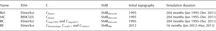
Ref., the reference simulation; MC, the experiment designed to investigate the sensitivity of transient behavior to model choice; BC, the experiment designed to investigate the sensitivity of transient behavior to basal boundary condition (C); BE, the experiment designed to investigate the possible mechanism triggering the drastic acceleration of the southern part of Basin 3 starting from autumn 2012.
In addition, we also carried out simulations to investigate the role of changing basal friction in the recent surge in southern Basin 3 that started in autumn 2012. We use the mean 1990–2000 SMB field projected by IDW as climatic forcing since we do not have SMB time series from the RCM for this time period.
4.1. Reference transient simulation
The reference simulation is performed with the full-Stokes IDM Elmer/Ice and employs the topographically corrected SMB field (SMB elevcorr ). We choose a time evolving scenario for the friction coefficient, C linear , which prescribes the locally linear temporal transition between C 1995 and C 2011 (from 1995 to 2011). We think that this combination stands for the best available choice for transient simulations of Basin 3 with the given input data; however, we cannot claim that this represents the most realistic simulation due to the lack of the representations of certain physical processes in the model, which will be discussed in Section 5.
Figure 3 shows the absolute and relative error between the modeled and post-processed observational surface flow speed (Fig. 1e) over Basin 3 at the end of the transient simulation in 2011:
 $$\varepsilon = \left \vert {u_{\bmod}} \right \vert - \left \vert {u_{obs}} \right \vert, $$
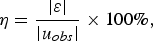 $$\eta = \displaystyle{{\left \vert \varepsilon \right \vert} \over {\left \vert {u{}_{obs}} \right \vert}} \times 100\%, $$
where ε and η are the absolute and relative errors respectively, u mod is the modeled surface velocity and u obs is the observational surface velocity.

Fig. 3. (a) The absolute and (b) relative error between the modeled and observed surface flow speed at Basin 3 in 2011. The gray solid line marks Basin 3.

Fig. 4. The volume change of (a) Austfonna ice cap and (b) the outlet glacier in Basin 3 over time.
Relative errors are lowest over the fast flowing area. The errors are mainly introduced by the inverted basal friction coefficient as the fast flow is mainly due to basal sliding with ice deformation accounting for only ~5 m a−1 over Austfonna (Dowdeswell and others, Reference Dowdeswell, Unwin, Nuttall and Wingham1999). The simulated volume change rate in water equivalent (w.e.) of the entire ice cap for the period 2002–08 is −0.45 km3 a−1 (w.e.) (Fig. 4). However, the observed volume change rate is −1.3 ± 0.5 km3 a−1 (w.e.) (Moholdt and others, Reference Moholdt, Hagen, Eiken and Schuler2010) when taking into account the ice loss of ~1.4 km3 a−1 (w.e.) caused by rapid retreat of the calving front (Dowdeswell and others, Reference Dowdeswell, Benham, Strozzi and Hagen2008). The difference between the observations and the model results is therefore likely to be caused by a fixed-front calving criterion, that is, the calving front can neither advance nor retreat, and the thickness of the calving front is set in balance with the hydrostatic pressure from the ocean. Thus the contribution of calving flux to mass loss calculated here only accounts for the ice flux towards the calving front that is not related to front advance or retreat, which in the case of the simulation of Basin 3 means a thickening of the calving front. Treatment of calving is a difficult problem, though progress may be made by considering discrete-particle simulations of the ice fracture process (Åström and others, Reference Åström2013) with realistic geometry. From January 2002 to December 2011 the simulated volume loss of Austfonna is ~8.6 km3 of which ~32% comes from Basin 3.
4.2. Sensitivity to model choice
Figure 5 shows the modeled surface flow speed of Basin 3 at the end of the MC simulation (Table 1) as well as the reference simulation. The location of the fast flowing area is the same for both Elmer/Ice and BISICLES because the same initial geometry and time-evolving C fields are used. BISICLES produces relatively higher flow velocities close to the calving front of the northern outlet. The divergence between the two models as the simulation progresses can be clearly seen in the flow line snapshots in Figure 6. The BISICLES surface flow speeds gradually surpass those of Elmer/Ice after ~120 months (in January 2005) but only become significantly higher in the final 12 months (January–December 2011). In other words, BISICLES is more sensitive to decreasing C than Elmer/Ice.

Fig. 5. The modeled surface flow speeds in December 2011 given by (a) Elmer/Ice, (b) BISICLES for the MC simulation (Table 1) (color bar on the left; in m a−1) and (c) the difference between BISICLES and Elmer/Ice (the reference) modeled surface flow speeds (color bar on the right; in m a−1). The gray solid line marks Basin 3.

Fig. 6. (a) The modeled speed and (b) surface elevation change simulated by Elmer/Ice (red) and BISICLES (blue) along the white flow line (Fig. 2) for the MC simulation in January 2005 (dashed line), January 2010 (solid line) and December 2011 (dotted line). The black solid line shows the modeled speed in 1995.
The mass loss over the entire Austfonna ice cap in BISICLES simulations exceeds that of Elmer/Ice by 2.25 km3 by the year 2011. However, mass loss from Basin 3 is less in BISICLES than in Elmer/Ice. BISICLES produces thicker ice at the calving front than Elmer/Ice (Fig. 6), but as both models use the same fixed-front calving scheme, the difference in mass flux may be from surface elevation feedbacks that differ due to the different simplification of the stress balance equation adopted in these two models.
4.3. Sensitivity to basal friction coefficient
Earlier studies using inverse methods (Gillet-Chaulet and others, Reference Gillet-Chaulet2012; Gladstone and others, Reference Gladstone2014; Schäfer and others, Reference Schäfer2014) have shown that a spatially variable basal friction coefficient was needed to reproduce the observed surface velocities over complex terrains. The observational surface velocity fields show a significant acceleration of Basin 3 from 1995 to 2011, and the recent observations of a full surge show that acceleration continued until at least 2013 (Dunse and others, Reference Dunse, Schuler, Hagen and Reijmer2012, Reference Dunse2015). To capture the change of the velocity field in a transient simulation, temporal change of the C field based on knowledge of the underlying physical processes would be required. Lacking a process-based model that computes the temporal evolution of the basal friction conditions based on factors such as basal hydrology (Gladstone and others, Reference Gladstone2014), we evolve the basal friction field in two further ways, constrained by the inversions obtained for 1995 (C 1995) and 2011 (C 2011). Keeping other conditions the same as for the reference simulation, we vary the C field using the scenarios employed in the BC simulations (Table 1) over the 204 months period:
C step1995 : Use C 1995 for the first 192 months (January 1995–December 2010) and instantaneously switch to C 2011 for the rest (January 2011–December 2011);
C step2011 : Use C 1995 for the first 12 months (January 1995–December 1995) and instantaneously switch to C 2011 for the rest (January 1996–December 2011).
Figure 7 shows snapshots of the evolution of the surface flow speed along the flowline (Fig. 2). The abrupt change in basal friction coefficient distribution in both C step2011 and C step1995 brings about a corresponding change in the velocity (in 1995 in the first case and 2011 in the second), with flow velocities speeding up by a factor of four near the calving front. At the same time, a linear transition from C 1995 to C 2011 (C linear ) leads to a temporally smooth transition between the 1995 and 2011 flow speeds. The difference between these simulations by 2011 is far less pronounced: the most obvious difference is slower flow near the front – ~600 m a−1 – in C step2011 compared with 800 m a−1 in the other two cases, due to the longer period of elevated discharge and hence a lower surface elevation by 2011. Observations of Basin 3 since 2008 (Dunse and others, Reference Dunse2015) exhibit partially reversible stepwise multiannual acceleration of Basin 3; these are sudden speedup events coincident with the summer melt seasons, each of which requires rapid changes of the basal condition (C distribution) for the fast flowing area.

Fig. 7. As for Figure 6 but for the reference and BC simulations (Table 1). (a) Modeled speed and (b) surface elevation change of C linear (red), C step1995 (brown) and C step2011 (blue) in January 2005 (dashed lines), January 2010 (solid line) and December 2011(dotted lines). The black solid line shows the modeled speed in 1995.
In the experiment deploying C step2011, a dramatic mass loss occurs after the C field is switched which exceeds that of the reference simulation by a factor of 2.6 by the end of the simulation. On the other hand, the volume loss for the whole of Austfonna under the C step1995 scenario is 1.8 km3 less than C step2011 scenario (Fig. 4).
4.4. The role of friction coefficient in the recent acceleration of southern Basin 3
Inspired by the sensitivity tests and the recently published observations (Dunse and others, Reference Dunse2015) we carried out additional simulations to investigate the role of changing basal friction in the recent surge in southern Basin 3 that started in autumn 2012, by linearly extrapolating the evolution of the C field obtained for the year 2011 over Basin 3 using the C 1995 to C 2011 time gradient for each point. We also changed the initial values of C in two different regions of the southern part of Basin 3 (Fig. 8) to a relatively low friction condition (C = 10−4 MPa a m−1) while keeping the northern part the same as the inverted value from 2011 velocity. We then linearly reduced C of the southern low friction area to a near zero friction condition (C = 10−30 MPa a m−1) over the course of the simulation. Thus three simulations are carried out for the 17 months from January 2012 to June 2013 (Table 1):
-
• C linearextrap : Linearly extrapolate C for only Basin 3 starting from C 2011 between January 2012 and June 2013 using the C 1995 to C 2011 gradient and constrained by a minimum value of 10−30 MPa a m−1 and keep C 2011 elsewhere;

Fig. 8. The exponent (β) of linearly extrapolated basal friction coefficient (C). The color-coded map shows the β from the reference simulation in February 2013 where the dark blue corresponds to the minimum values C = 10−30 MPa a m−1. The area confined by the blue and pink dash-dotted lines indicate the region where C is initially changed to 10−4 MPa a m−1 and reduced to 10−30 MPa a m−1 from January 2012 to June 2013 in C nofrc1 and C nofrc2 cases, respectively. The gray solid line marks Basin 3.
-
• C nofrc1 : Linearly change C from a spatially homogeneous value of 10−4 MPa a m−1 to 10−30 MPa a m−1 between January 2012 and June 2013 for the area between the blue line and the calving front in Figure 8, while keeping C 2011 elsewhere. The area where C nofrc1 is applied matches the area in the southern Basin 3 where the sudden acceleration in April 2012 was observed (Dunse and others, Reference Dunse2015);
-
• C nofrc2 : As for C nofrc1 but for the larger area, between the pink line and the calving front in Figure 8, and keep to C 2011 elsewhere.

The linear extrapolation reduces C in most of the northern fast flowing units to close to 10−30 MPa a m−1 within 12 months. Consequently, the formerly fast flowing unit in the northern part of Basin 3 accelerates dramatically to ~6400 m a−1 (17 m d−1) by the end of the simulation, which is comparable with the observed maximum surging speed in 2013 (20 m d−1) (Dunse and others, Reference Dunse2015). This near zero basal shear stress (i.e. minimal basal frictional drag) most resembles the situation of ice separated from its bedrock due to the presence of basal water at, or exceeding, full ice overburden pressure (Weertman, Reference Weertman1957; Kamb, Reference Kamb1970, Nye, Reference Nye1970). However, the southern part of Basin 3 only accelerates to ~90 m a−1 (0.25 m d−1) by January 2013 (Fig. 9). This is because the low friction area in southern Basin 3 is rather far inland and certainly cannot produce the observed acceleration near the terminus. Thus a simple continuation of the C 1995 to C 2011 basal friction trend and spatial pattern cannot reproduce the sudden acceleration of southern Basin 3.

Fig. 9. The modeled surface flow speed in January 2013 for (a) C linearextrap, (b) C nofrc1 and (c) C nofrc2.
By reducing C from 10−4 MPa a m−1 to 10−30 MPa a m−1 close to the terminus in the southern part of Basin 3 (the pink and blue areas in Fig. 8) we manage to produce a gradual acceleration there in both the C nofrc1 and C nofrc2 cases. This behavior is not produced unless the initial value of C in the pink or blue areas is reduced from the C 2011 values to 10−4 MPa a m−1. Although the modeled surface flow speed of the C nofrc1 case in February 2013 is comparable with the maximum observed surging speed, the acceleration does not spread across the entire basin (Fig. 9b). Several tests with various larger areas with reduced basal friction in southern Basin 3 have been carried out (not shown), but only the distribution defined in C nofrc2 can produce an accelerating area that is comparable with the observed basin-wide surge area. In the C nofrc2 case, where the imposed low-friction region overlaps with that of the fast flowing northern flow unit, the acceleration expands to the entire basin but leads to higher velocities than the maximum observed surging speed (Fig. 9c).
5. DISCUSSION AND CONCLUSIONS
Observations of the outlet glacier in Basin 3, Austfonna revealed a discrete, multiannual stepwise acceleration in its northern basin since 2008 (Dunse and others, Reference Dunse2015) as a continuation of a gradual acceleration started in 1991 (Dowdeswell and others, Reference Dowdeswell, Unwin, Nuttall and Wingham1999), followed by a recent sudden speedup of its southern basin starting in early 2012 (Dunse and others, Reference Dunse2015). We investigated how different representations of the temporal evolution of the spatial basal friction coefficient succeed in capturing the evolving dynamics of Basin 3, i.e., ice volume change in Austfonna over a period of 17 years and 40-fold changes of the surface flow speed. We also compare the influence of ice dynamics and volume change by using different IDMs.
The comparison between the results from the studies indicated by ‘MC’ and ‘BC’ (Table 1) clearly shows that the dynamic response of the fast flowing area in Basin 3 in the model simulations is governed by the temporal evolution of basal friction coefficient. Ice volume flux and sea-level rise contribution also depend most strongly on the choice of the basal friction coefficient evolution. As mentioned earlier, the choice of SMB downscaling method has no significant impact over the 17 years of simulation time. Similarly, the model physics, with both models including horizontal normal and shear stresses, appears to be less critical.
The BISICLES IDM produces generally higher flow speeds over Basin 3 than the Elmer/Ice model when using the same basal friction coefficient field. That is consistent with the results in experiment P75D of the MISMIP3d model intercomparison showing that BISICLES produces slightly higher flow speed than Elmer/Ice when using the same initial conditions in the steady-state simulations (Pattyn and others, Reference Pattyn2013). The differences could be due to the additional stress components in the full-Stokes equation solved by Elmer/Ice, namely the bridging stresses, which produce more buttressing from the fast flowing outlet units, but could also be related to the inclusion of simplified (and over estimated) vertical shear strains in the effective viscosity. As the basal friction coefficient field is inverted in the fullStokes IDM, this effect will have been partially prescribed in the BISICLES simulation. The complex geometry used in the simulation may also create inconsistencies via non-physical factors such as interpolation schemes or the numerical methods employed by the two IDMs.
Although the response of the modeled ice flow in Basin 3 is insensitive to the different SMB downscaling methods we used in these specific decadal timescale transient simulations, the SMB-elevation gradient method we favoured – and which did produce a more realistic SMB distribution – is designed to allow asynchronous coupling of a RCM with an IDM. The advantages of the method should be more noticeable in steep topography, for example in many coastal regions, or over millennial periods such as glacial/interglacial transitions (Helsen and others, Reference Helsen, van de Wal, van de Broeke, van de Berg and Oerlemens2012; Schäfer and others, Reference Schäfer, Möller, Zwinger and Moore2015). The choice of the RCM downscaling method may also become crucial when linking the process of surface melt to basal hydrology in future model development.
Previous studies (Dunse and others, Reference Dunse, Greve, Schuler and Hagen2011, Reference Dunse2015; Gladstone and others, Reference Gladstone2014) addressed the importance of both basal processes and the climatic driving force acting on the ice upper boundary (specifically, surface melting) in explaining the underlying physics of the surge in Basin 3. In our study, the governing effect of basal friction coefficient on both modeled velocities and volume change indicates the need for a process-based subglacial component to alter the basal friction through time regardless of the choice of IDMs. A soft-bed mechanism that involves the basal hydrology system and till deformation could be a future model development that may explain the surge in northern Basin 3 (Gladstone and others, Reference Gladstone2014). In addition the missing link between climatic driving force and basal sliding, namely the representation of processes for routing surface meltwater down to the glacier bed in IDMs, would improve our ability to evaluate the impact of surface boundary condition changes (climate forcing) on model results.
Simply preserving the basal friction coefficient spatial pattern in our simulations cannot reproduce the observed surge acceleration pattern spanning from January 2012 to June 2013. Hence, the models require some method of specifying how basal friction changes during the course of the surge itself as a result of certain feedback mechanisms.
Furthermore unlike the stepwise acceleration of the northern unit that has lasted two decades, the abrupt speedup in the southern basin could be initiated by a different mechanism, which might be linked to the changes in the terminus. Future model development about ice front migration might be needed. The bed topography profile (Fig. 1) shows that the southern and middle flow units rest on a relatively flat or even on slightly reversed slopes. In contrast the northern basin has an undulating bed, which would likely lead to contrasting basal hydrology and roughness and thus to differences in calving front migration such as a marine ice-sheet instability (Schoof, Reference Schoof2007). This emphasizes the importance of accurate coastal bedrock topography in future simulations of calving front migration. Last but not the least, it is clear that the eventual basin-wide surge is a result of the merging of the southern fast flowing unit with the northern one.
ACKNOWLEDGEMENTS
We wish to thank all the partners for providing data and constructive discussion during the study, especially Ruth Mottram from Danish Meteorological Institute for the HIRHAM5 surface mass-balance time series, Tazio Strozzi from GAMMA Remote Sensing and Consulting AG for the remotesensing surface velocity data, Thomas Schuler from the University of Oslo for the September 2003 to August 2004 reference surface mass-balance data and Thorben Dunse from the University of Oslo for the bedrock and surface elevation data. We wish to thank Fabien Gillet-Chaulet from Laboratoire de Glaciologie et Géophysique de l'Environnement for making available his code for the inverse modelling. We also acknowledge CSC–IT Center for Science Ltd. for the allocation of computational resources. Yongmei Gong is funded by project SVALI and European Science Foundation project Micro–DICE. This publication is contribution No. 74 of the Nordic Centre of Excellence SVALI funded by the Nordic Top–level Research Initiative. Rupert Gladstone is funded from the European Union Seventh Framework Programme (FP7/2007–2013) under grant agreement no. 299035.


 Open access