


Introduction
Ekström Ice Shelf (Ekströmisen) covers an area of ∼8700 km2 (extracted from IfAG, 1989) and is one of the comparatively small ice shelves in the coastal zone of northern Dronning Maud Land, Antarctica. The dome-shaped ice cap Halvfarryggen and Atka Ice Rise, which borders Atka Iceport in the south, subdivide the ice shelf into a small eastern part (∼2000 km2) and a major western part (Fig. 1). The latter is bounded by the Ritscherflya ice-sheet region to the south and by the Sorasen and Austasen ice caps to the west. Both of these show an individual flow regime largely independent of the movement in the adjacent ice-sheet region (IfAG, 1989).
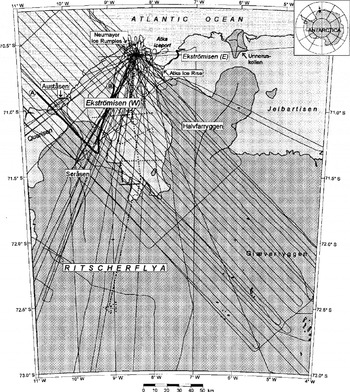
Fig. 1. Ekström Ice Shelf (Ekströmisen) and adjacent ice-sheet and tee-shelf regions with aerial-survey tracks from 1983/84,1985/86 and 1988/89 seasons. Profile A-B is shown in Figure 2. The ground traverse with geodetic levelling (Reference Moller and RitterMöller and Ritter, 1988; Reference Karsten, Ritter, Miller and OerterKarsten and Ritter, 1990) is marked with dotted lines (base map here and on subsequent figures from IfAG/AWI, 1994).
Within the framework of a long-term project, the Institut fur Geophysik der Universität Munster carried out extensive aerial surveys (altimetry, radio-echo sounding) over Ekström Ice Shelf and the adjacent ice-shelf and ice-sheet areas. The data from the 1983/84 and 1985/86 field seasons, together with geodetic ground levelling (Reference Moller and RitterMoller and Ritter, 1988; Reference Karsten, Ritter, Miller and OerterKarsten and Ritter, 1990), were used to derive maps of surface topography and ice thickness for the western part of Ekström Ice Shelf and the eastern slope of Sorasen (Reference Thyssen and GrosfeldThyssen and Grosfeld, 1988; IfAG, 1989). On the basis of these datasets, Reference Hoppe and ThyssenHoppe and Thyssen (1988) evaluated the subglacial-bedrock topography of large parts of Ritscherflya.
In 1988/89, the database was increased by measurements of 22 additional flights from about 25 000 km of flight tracks in total. The complete coverage is shown in Figure 1.
The processing of the combined datasets yielded new detailed maps of surface and bedrock topographies and of the ice thickness. These maps cover the whole drainage system formed by Ekström Ice Shelf and its catchment area. In addition, characteristic vertical cross sections are discussed. An estimate of the mean annual mass discharge over the grounding line is given.
Processing of the Aerial Measurements
The aircraft used were equipped with an inertial navigation system (INS) to fix the actual geographical position, barometric and radar altimeters to record the flight altimetry data, and a radio-echo sounding (RES) system which emits electromagnetic wave trains and records the travel-times of the reflected signals from the surface and the bottom of the ice (cf Reference Thyssen and KohnenThyssen, 1985; Reference Thyssen, Bombosch and SandhagerThyssen and others, 1993). The INS was calibrated before each flight with the known station coordinates. Both altimeters were usually adjusted over the open ocean after each take-off.
An irregular drift of the INS necessitated a correction of the navigational data. This was performed by applying a correlation procedure based on prominent topographic structures like ice fronts, grounding lines, ice divides or ice-free mountain outcrops (nunataks), whose geographical positions were well-known from satellite-image analyses (IfAG/AWI, 1994), and which also could be identified unambiguously in the altimetry data and/or the RES records. With this procedure, the mean location error of the individual measuring points was reduced to about ±2 km. The corresponding error tolerances for measuring points located in ice-sheet regions without any significant surface features may be considerably larger.
Ice-surface elevations were calculated from the flight altimetry data, which had also been corrected before (cf. Reference Thyssen and GrosfeldThyssen and Grosfeld, 1988). From the RES records the travel-time differences of the electromagnetic wave trains reflected from the ice surface and from the ice-bedrock (or ice-sea-water) interface were determined and converted to ice thicknesses using a velocity-depth function (Reference BlindowBlindow, 1986). Subglacial-bedrock elevations were derived from the difference between ice-surface elevations and ice thicknesses.
A typical RES profile, obtained in 1988/89 over the north-western part of the investigated area, is shown in Figure 2a. Besides the reflections from the ocean and ice surfaces and the ice-bedrock and ice-sea-water interfaces several additional structures are resolved, which are caused by diffractions of the electromagnetic waves (cf Reference Thyssen, Bombosch and SandhagerThyssen and others, 1993). Figure 2b shows the accompanying cross section based on the fully processed dataset. The grounded ice domes Sorasen and Austasen now stick out clearly against the flat ice-shelf regions, where measured depths of the ice-shelf base largely agree with depths calculated from ice-surface elevations and a hydrostatic relation similar to that found by Reference Thyssen and GrosfeldThyssen and Grosfeld (1988). Close to the grounding lines the surface elevations of Ekström Ice Shelf and the adjacent Quarisen ice shelf are up to 6 m too low to be hydrostatically balanced by the measured ice thicknesses. This phenomenon has been observed in different grounding zones of several ice shelves (eg. Reference StephensonStephenson, 1984) and is caused by a slight flexure of the ice body seaward of the grounding line, before it returns to hydrostatic equilibrium.
Fig. 2. (a) RES profile from the northwestern part of the investigated area (recorded in 1988/89 at approximately constant altitude). Besides reflections from the ice (SI) and ocean (S2) surfaces, and from ice-bedrock (Bl) and ice-sea-water (B2) interfaces, additional structures are resolved, which are caused by diffraction of electromagnetic waves by crevasses (C), rifts (R) and internal layers (I). Different multiples (M) are visible. The position of the profile is marked in Figure 1. Seabed topography is not determinable with RES surveys, (b) Accompanying cross section based on the fully processed dataset. Relief of ice-shelf base, as calculated from ice-surface elevations and a hydrostatic relation, is indicated by broken lines.
To derive three digital geometric models, which describe the surface and subglacial-bedrock topographies and the ice-thickness distributions in the whole investigated area, the measuring points of the geometric quantities along the flight tracks were interpolated on regular horizontal grids. Those parts of the digital-terrain model, representing ice-sheet regions with only a sparse data coverage or an inadequately corrected database, were post-processed by applying smoothing and other filtering operations. The final horizontal resolution of each digital geometric model is about 725 m × 725 m. The estimated local error tolerances for the different geometric quantities are given in Table 1.
Table 1. Error tolerances for the three geometric quantities in the corresponding digital models. The local differences result from the irregular distribution of measuring points and from the varying effectiveness of the applied correction methods
Ice-Surface Topography
The new digital-terrain model has been used to derive an improved topographic map of Ekström Ice Shelf, its catchment area, and parts of the adjacent ice-sheet and ice-shelf regions (Fig. 3). On Halvfarryggen, Sorasen, and Austasen the lateral boundary of the drainage system directly coincides with the crests or central ice divides of these ice domes. In the Ritscherflya ice-sheet region the boundary approximately follows the steepest surface slope, because the latter generally corresponds with the mean horizontal flow direction of grounded ice masses (Reference PatersonPaterson, 1969, p. 64–65). With that, the total extension of the catchment area of Ekström Ice Shelf is estimated to be ∼20500 km2.
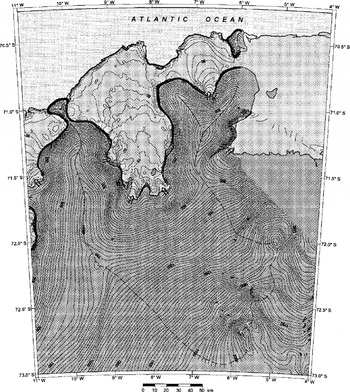
Fig. 3. Ekström Ice Shelf and adjacent ice-sheet and ice-shelf regions (elevations in m.a.s.l). Contour intervals change at 100 mfrom 5 mto 25 m. The boundary of the drainage system coincides with crests of ice domes and continues southwards approximately along the steepest surface slope in the Ritscherflya ice-sheet region (broken line). Arrows indicate zones of high ice flux from island into the ice shelves.
Figure 3 shows that both Halvfarryggen and Austasen include a prominent summit rising to about 675 m and 250 m, respectively, while the Sorasen ice dome is crowned by a 50 km-long crest at altitudes of 725–750 m. A maximum surface elevation, >2200 m a.s.L, is attained in the southern part of the drainage system. To the northwest, the elevation of the ice surface then decreases with a mean gradient of about –15 m km−1 to ∼100 m near the grounding line.
The surface relief of the transitional areas, including grounded and floating ice, indicates that the mass discharge from inland into the Ekström Ice Shelf is mainly concentrated in four relatively narrow zones. Through two of these zones, ∼10 km and ∼16 km wide at the grounding line, the Ritscherflya ice-sheet region drains into the southernmost part of the ice shelf. Furthermore, an essential part of the ice outflow from the eastern slope of Sorasen occurs over a ∼ 2 0 km long section of the southwestern grounding line of Ekström Ice Shelf. Through the fourth of the particular zones of concentrated ice flux, the eastern part of the ice shelf is fed by ice masses emanating from its main catchment area, the ∼1400 km2 large northern slope of Halvfarryggen.
The ice-shelf region south of Atka Ice Rise, with a mean surface elevation of ∼ 3 5 m, can be assigned neither to the western nor eastern part of Ekström Ice Shelf. The conclusion is that both parts, together with their catchment areas, represent largely independent ice-sheet-ice-shelf systems with individual geometric characteristics and flow regimes.
Ice-Thickness Distribution and Subglacial-Bedrock Topography
The digital geometric models yield new detailed maps of ice-thickness distribution and subglacial-bedrock topography in the region of Ekström Ice Shelf and its catchment area, which are displayed in Figures 4 and 5, respectively.

Fig. 4. Ice-thickness distribution in Ekström Ice Shelf area and adjacent ice sheets and ice shelves (ice thicknesses in m). Contour interval is 100 m. The two darkest-grey shadings indicate regions where thickness exceeds 700 m and 1000 m, respectively. The broken line marks the southern boundary of the Ekström Ice Shelf catchment area.

Fig. 5. Subglacial-bedrock topography of ice sheets and ice domes adjacent to Ekström Ice Shelf ( bedrock elevations in m a.s. I.). Contour line interval is 250 m. Areas with ice grounded below –500 m are shaded in light grey; regions with bedrock above sea level in dark grey. The broken line marks the southern boundary of the Ekström Ice Shelf catchment area. Arrows indicate zones of high ice flux from inland into the ice shelves.
The subglacial bedrock in the southeastern part of the drainage system shows distinctive mountainous structures with differences in altitude exceeding 1000 m over horizontal distances of less than 5 km in places. Due to the relatively smooth ice surface, similarly significant variations in ice thickness can be observed. In several areas of subglacial depressions, the thickness of the ice sheet exceeds 1500 m, locally even 2000 m. In contrast, the southwestern part of the Ekström Ice Shelf catchment is characterized by a considerably less-undulating bedrock surface. The mean thickness of the ice sheet here has been estimated at ∼850 m. The maximum ice thickness (> 1500 m) occurs about 20 km south of the grounding line. Here, the deepest depression of the subglacial bedrock within the investigated area has been found, where the ice-bedrock interface is more than 1000 m below sea level. In the whole southern part of the drainage system the bedrock surface is above sea level. Some mountain outcrops penetrate the ice cover and rise to 1800 m a.s.l.
The Halvfarryggen, Sorasen, and Austasen ice domes are grounded on a slightly undulating bedrock surface at a mean depth of ∼250 m, but locally rising up to ∼100 m below sea level (cf. Fig. 2b and 6). The ice-bedrock interface mostly inclines from the centres of the ice domes towards their grounding lines, where depths of more than 500 m below sea level are reached, particularly in areas of subglacial depressions. The relatively smooth surface relief of the bedrock below the ice domes probably results from former glacial erosion.

Fig. 6. Vertical cross sections of Ekström Ice Shelf and its catchment area, (a) Profiles A-A′, (b) B-B′and (c) C-C coincide with the 200, 800 and 1400 m contour lines, respectively, and are oriented almost perpendicular to the horizontal/low direction of the grounded ice masses. Profile D-D′ ( d) follows a flowline from the southeastern boundary of the drainage system to the ice front. Arrows indicate subglacial depressions with high ice flux from inland into the ice shelf Inset map (e) shows positions of profiles and four additional flowlines of Ritscherflya (broken lines).
The map of subglacial-bedrock topography (Fig. 5) additionally indicates that the four particular zones of concentrated ice flux from inland into the ice shelf, identified in the ice-surface topography, coincide with significant graben-like depressions in the ice-sheet base. Their depths generally increase with decreasing distance from the grounding line and range approximately between 300 m and 900 m. In the areas of the subglacial depressions, which are 10–30 km wide and extend over 20 km to more than 50 km from the grounding line in the adjacent ice-sheet regions, the ice-thickness distribution reaches local maximums of 700–1600 m.
Besides the four zones of increased ice discharge from inland into Ekström Ice Shelf (indicated as arrows on the map), two additional zones can be identified in the new maps. The latter characterize the flow regimes of the adjoining Quarisen and Jelbartisen ice shelves and their catchments. These zones also coincide with subglacial depressions, inclining towards the corresponding grounding lines (Fig. 5).
By numerical integration of the digital ice-thickness model, the volumes of Ekström Ice Shelf and its catchment area have been determined to be ∼3200 km3 and ∼16 000 km3, respectively. Calculating the mean density of the ice column as a function of its thickness (cf Reference Thyssen and GrosfeldThyssen and Grosfeld, 1988), the total ice mass stored in the drainage system can be estimated to be ∼17 000 Gt.
Selected Profile Sections
Based on the assumption that movement takes place approximately along the steepest surface slope in grounded regions (cf. Reference PatersonPaterson, 1969, p. 64–65), the digital geometric models have been used to determine four selected vertical cross sections of Ekstrom Ice Shelf and its catchment area (Fig. 6). Since the profiles A-A′, B-B′ and C-C′ coincide with the 200, 800 and 1400 m contour lines, respectively, the accompanying cross sections are oriented almost perpendicular to the horizontal flow direction of the grounded ice masses. In contrast to that, the orientation of the fourth cross section, D-D′, is approximately parallel to the flow direction, because the corresponding profile represents a flowline from the southeastern boundary of the catchment area to the ice-shelf front west of Neumayer Ice Rumples. The inset map in Figure 6 shows that profile D-D′ intersects the three others, at the points D1400, D800 and D200, before it crosses the grounding line and a small ice rumple within the ice shelf, where the course of the profile has been selected according to flowlines in the glaciological map from HAG (1989).
The vertical cross section A-A′ (Fig. 6a) reflects the main characteristics of the ice-thickness distribution and the subglacial-bedrock relief near the grounding line of Ekström Ice Shelf. Above all, the four graben-like depressions in the bedrock topography clearly stick out, which have been identified to coincide directly with zones of concentrated ice flux into the ice shelf. As the lateral distances between the selected flowlines of the Ritscherflya ice-sheet region significantly decrease towards the north, a convergent mass flux seems to predominate even in extensive parts of the southern catchment area. Furthermore, the comparative smoothness of bedrock surface below the Sorasen and Halvfarryggen ice domes becomes evident from Figure 6a.
The cross sections B-B′ and C-C′ (Fig. 6b and 6c) show the difference in large-scale bedrock roughness between the southwestern part of the drainage system, where only few significant local undulations of the ice-sheet base occur, and the southeastern part, where the ice masses are grounded on prominent mountainous structures. With increasing distance from the grounding line towards the southeast, this subdivision of the subglacial-bedrock relief clearly gains in significance. Since the bedrock surface is simultaneously ascending with a mean gradient of ∼ 15 m km−1, the ice-bedrock interface in the southern part of the Ekström Ice Shelf catchment slopes down below sea level only within deep subglacial depressions. In the southeastern part the ice sheet is penetrated by several mountain outcrops 1570–1950 m high (IfAG, 1993), one of them being depicted in the cross section C-C′ at profile distance 72 km.
Along the profile D-D′ (Fig. 6d) the gradient of the ice-sheet surface varies from - 5 to –30 m W 1. The surface relief reflects the repressive effect of the subglacial mountainous structures on the movement of the ice-sheet. Hence, especially in the southeastern part of the drainage system, small-scale changes in flow velocity and a comparatively complex state of stress within the ice body are to be expected. Between profile distances 107 km and 128 km near the grounding line, the ice surface shows a concave shape, pointing to an accompanying flow regime similar to that of an ice stream (Reference BentleyBentley, 1987). Thus, the concentrated ice flux towards the southeastern grounding line of Ekström Ice Shelf might be connected with basal-sliding processes. Nearly the same ice-dynamic situation is expected to prevail inland of the grounding zone adjacent to the west (Reference MayerMayer, 1996).
The decrease in ice-shelf thickness, by - 400 m between the grounding line and the small ice rumple at the profile distance 145 km, is supposed to result mainly from strong basal melting (Reference KipfstuhlKipfstuhl, 1991). Further north up to profile distance 193 km, the mean decrease in ice thickness significantly reduces to ∼1.5 m km−1. Here, the prominent parts of Sorasen and Halvfarryggen cause a slight lateral compression of the ice shelf (Reference Moller and RitterMoller and Ritter, 1988; IfAG, 1989). Additionally, the basal-melt rates have been estimated to be only a few tens of centimetres per year in this region (Reference KipfstuhlKipfstuhl, 1991). Again further north, the ice flow is now strongly influenced by general horizontal extension and increased basal melting, leading to a thinning of the ice shelf of ∼ 10 m km−1. Over the last 30 km of the profile, the total reduction in ice-shelf thickness is remarkably small, because restraint from the nearby Neumayer Ice Rumples restricts the spreading of the ice shelf and its horizontal flow velocity (Reference Moller and RitterMoller and Ritter, 1988; IfAG, 1989). This effect also seems to compensate for the influence of basal-melt rates of ∼ 1 m a−1 (Reference KipfstuhlKipfstuhl, 1991; Reference Nixdorf, Oerter and MillerNixdorf and others, 1994; Reference Lambrecht, Nixdorf, Zurn and OerterLambrecht and others, 1995) on the ice-thickness distribution in the coastal zone. Obviously, Neumayer Ice Rumples represent the pinning points of the western part of Ekström Ice Shelf and are of great importance for its stability and its present seaward extension.
Discussion and Conclusions
Aero-geophysical measurements have yielded new digital geometric models for ice-surface and subglacial-bedrock elevations and ice thicknesses of Ekström Ice Shelf and its whole catchment area. The models have been used to derive improved maps for the drainage system and to determine the horizontal extensions of its different ice-sheet and ice-shelf regions as well as the volume and the mass of the ice stored in each of these parts. In addition, the geometric datasets represent essential input data especially for numerical model calculations. In that way, the basic ice-dynamic parameters of the coupled ice-sheet-ice-shelf system might be quantified in future. These are, above all, the flow velocity of the ice masses, the temperature regime, and the states of strain and stress within the ice body.
Although precise determination of the characteristic mass-balance quantities of the drainage system requires knowledge of the ice-mass velocity flow-field (cf., e.g., Reference PatersonPaterson, 1969, p. 148, 152), one of these quantities, the mean annual mass discharge from inland into the ice shelf, can be estimated on the basis of the geometric datasets together with measured surface-accumulation rates.
The main catchment areas of the western part of Ekström Ice Shelf are the eastern slope of Sorasen (∼2050 km2), the northeastern regions of Ritscherflya (∼15 200 km2), and the western slope of Halvfarryggen (∼1900 km2). In-situ measurements of the mean annual snow accumulation (Reference Oerter, Graf, Schlosser and OerterOerter and others, 1997; personal communication from H. Oerter, 1998) and long-term meteorological observations (Reference König-LangloKönig-Langlo, 1992; Reference Konig-Langlo and HerberKönig-Langlo and Herber, 1996), which show easterly winds predominating in the coastal zone of Ekström Ice Shelf and pointing to an increased surface accumulation on windward slopes, yield estimated values for the mean surface-accumulation rate in the three main catchment areas of about 0.3, 0.2 and 0.15 ma−1 (ice equivalent), respectively. Presupposing steady-state conditions, neglecting mass loss due to melting at the ice-sheet base and assuming a constant ice density of 915 kg m−3, this rough quantification of the mass flux from Sorasen, Ritscherflya, and Halvarryggen into the western part of Ekström Ice Shelf results in ∼0.6, ∼ 2. 8 and ∼0.3 Gt a"1, respectively. Therefore, the whole annual ice outflow from inland over the grounding line into western Ekström Ice Shelf would add ∼3.7 Gt (or ∼0.3%o of the total ice mass stored in the accompanying catchment areas). Reference KipfstuhlKipfstuhl (1991) estimated a mass flux over the grounding line of only ∼2.6 Gt a−1, but obtained an unexplained deficit of ∼l.5Gta−1 in his mass-balance determination for the western part of Ekström Ice Shelf.
The mean horizontal flow velocity within the southern grounding zone is ∼144ma−1 if the width of the zone, the mean ice thickness, and the ice flux are assumed to be 25 km, 850 m and 2.8 Gt a−1, respectively. This is consistent with results of GPS measurements which have been carried out along a profile crossing the southwesternmost section of the grounding line and yielded surface velocities of about 160 ma−1 (Reference MayerMayer, 1996).
By means of an analogous estimate for the smaller eastern part of Ekström Ice Shelf, the mean annual mass discharge from the northern slope of Halvfarryggen into this part of the ice shelf and the mean flow velocity in the central grounding zone with concentrated ice flux are calculated to be ∼ 0.4 Gt and ∼100 m a"1, respectively. Due to the lack of in-situ glaciological measurements and the small number of flight tracks over this region, the uncertainties in this rough quantification are correspondingly large.
The detailed investigation of Ekström Ice Shelf and the adjacent ice-sheet and ice-shelf areas with RES and surface-elevation measurements revealed new insights into ice-thickness distribution, the morphological setting and the drainage there. The new digital geometric datasets also represent an outstanding base for detailed dynamic modelling of the region which will be essential for assessing this area for the planned EPICA drilling.
Acknowledgements
The aerial surveys of 1988/89 were supported by the Deutsche Forschungsgemeinschaft under grant TH168/20-1. We are grateful to F. Thyssen, the initiator of this project, to M. Jonas, who was involved in the field measurements with the co-author, and to the laboratories of the Institut fur Geophysik der Universität Münster for constructing the RES system. The datasets were processed through the "Dynamic Processes in Antarctic Geosystems Project", funded by the Bundesministerium fur Bildung, Wissenschaft, Forschung und Technology der Bundesrepublik Deutschland (contract No. 03PL016A).


