


1. Introduction
Convection driven by spatial temperature patterns exhibits properties fundamentally different from the classical Rayleigh–Bénard (RB) instability (Bénard Reference Bénard1900; Rayleigh Reference Rayleigh1916), as the latter deals with uniformly heated walls and the onset of instability is independent of Prandtl number  $Pr$ (Kelly & Pal Reference Kelly and Pal1978; Bodenschatz, Pesch & Ahlers Reference Bodenschatz, Pesch and Ahlers2000; Krishnan, Ugaz & Burns Reference Krishnan, Ugaz and Burns2002; Freund, Pesch & Zimmermann Reference Freund, Pesch and Zimmermann2011), while the former deals with non-uniformly heated walls with the formation of a horizontal temperature gradient and a strong effect of $Pr$ at the onset of instability (Lyubimov et al. Reference Lyubimov, Lyubimov, Morozov, Scuridin, Hadid and Henry2009; Hossain & Floryan Reference Hossain and Floryan2013b, Reference Hossain and Floryan2014, Reference Hossain and Floryan2015). It is known that reduction of $Pr$ strengthens the influence of spatial modulations (Hossain & Floryan Reference Hossain and Floryan2013a) but its effects on the secondary states are yet to be studied. Temperature patterns represent external forcing generating spatial modulations (primary convection) which, under certain conditions, transit to secondary states (Hossain & Floryan Reference Hossain and Floryan2013b). The results in these literature are limited to a single Prandtl number ( $Pr=0.71$) for which the primary response of the system consists of stationary convection rolls with the axis orthogonal to the heating wave vector. The structure of these rolls is determined by the heating intensity, as measured by the Rayleigh number $Ra$, and by the heating wavenumber $\alpha$. It is known that an increase of $\alpha$ leads to formation of a convection boundary layer near the heated wall with all spatial modulations confined to this layer. A conduction zone emerges above this layer and the fluid there sees its edge as a uniformly heated wall. Thus, the outer layer can be considered as a layer subject to RB instability.
Transition to the secondary states is driven by a competition between the spatial parametric resonance (Manor, Hagberg & Meron Reference Manor, Hagberg and Meron2008, Reference Manor, Hagberg and Meron2009) and the RB mechanism (Bénard Reference Bénard1900; Rayleigh Reference Rayleigh1916). The former one produces the locked-in states where the primary rolls have a sub-harmonic relation with the secondary structures, and the latter one produces states well described in the literature. A transition zone where neither of these mechanisms dominates leads to the formation of a range of commensurate states with widely different properties and appearance of soliton matrices (Lowe & Gollub Reference Lowe and Gollub1985; Hossain & Floryan Reference Hossain and Floryan2013b), as well as system frustration as multiple states of the system are possible (Nixon et al. Reference Nixon, Ronen, Friesem and Davidson2013). Many of the possible states cannot be predicted by the Bloch theory for periodic systems (Bloch Reference Bloch1928; Floryan & Inasawa Reference Floryan and Inasawa2021).
This analysis is focused in the first step on the identification of the primary system response to variations of  $Pr$ in the range from $10^{-2}$ to $10^3$ which covers values of $Pr$ which are of practical importance (Verzicco & Camussi Reference Verzicco and Camussi1999; Lyubimov et al. Reference Lyubimov, Lyubimov, Morozov, Scuridin, Hadid and Henry2009). It explores in the second step transition to secondary states, how the relative strengths of two instability mechanisms is affected by variations of $Pr$ and what its consequences are. In particular, we investigate how parametric resonance changes with $Pr$ and what is the range of $\alpha$ producing locked-in states. We investigate how the range of $\alpha$ where the RB mechanism dominates changes with $Pr$. Finally we explore the system responses for the range of $\alpha$ where both mechanisms are in balance, how the system responses change with $Pr$ and how various commensurate states are formed. Section 2 discusses the primary convection which represents the forced response of the fluid. Section 3 discusses transition to secondary states and various topologies emerging from the system bifurcation. Section 4 provides a summary of the main findings.
2. Primary convection
The analysis is carried out using a model problem, as shown in figure 1, consisting of a horizontal slot between two parallel walls extending to  $\pm \infty$ in the $x$-direction filled in with a Boussinesq fluid (Koschmieder Reference Koschmieder1993) and exposed to spatial periodic heating at the lower wall while keeping the upper wall isothermal. The lower ( $\theta _L$) and upper ( $\theta _U$) walls’ temperatures are
 \begin{equation} \theta _L (x) = \tfrac{1}{2} \cos(\alpha x),\quad \theta _U (x) =0, \end{equation}
where  $\alpha$ stands for the heating wavenumber, $\theta$ denotes the relative temperature, i.e. $\theta = T-T _{ref}$, $T$ denotes the temperature and $T _{ref}$ stands for the upper wall (reference) temperature. The fluid has thermal conductivity $k$, specific heat per unit mass $c$, thermal diffusivity $\kappa =k/\rho c$, kinematic viscosity $\nu$, dynamic viscosity $\mu$, thermal expansion coefficient $\varGamma$ and density $\rho$. Horizontal temperature gradients drive convective rolls. The resulting temperature field is split into conductive ( $\theta _c$) and convective ( $\theta _1$) components, i.e.
 \begin{gather} \theta (x,y) = Pr ^{{-}1} \theta_c (x,y) + \theta_1 (x,y), \end{gather}
 \begin{gather} \theta _c(x,y)=\frac{1}{4} \left [\frac{{\rm cosh}(\alpha y)}{{\rm cosh}(\alpha)} -\frac{{\rm sinh}(\alpha y)}{{\rm sinh}(\alpha)} \right ] {\rm e}^{{\rm i} \alpha x} +{\rm c.c.}, \end{gather}
where c.c. stands for the complex conjugate. The amplitude of temperature variations along the wall  $T _d$ is used as the conductive scale and $T _v = T _d \nu / \kappa$ as the convective scale – $T {_v}/ T _{d}=Pr$ with $Pr=\nu / \kappa$. The half-distance $h$ between the walls is used as the length scale, $U _{v} \nu /h$ as the (convective) velocity scale and $P _{v}=\rho U ^{2} _{v}$ as the pressure scale. The convective component is described by
 \begin{gather} \frac{\partial u _1}{\partial x} + \frac{\partial v _1}{\partial y} = 0, \end{gather}
 \begin{gather} u _1 \frac{\partial u _1}{\partial x} + v _1 \frac{\partial u _1}{\partial y} ={-}\frac{\partial p _1}{\partial x} + \nabla^2 u _1, \end{gather}
 \begin{gather} u _1 \frac{\partial v _1}{\partial x} + v _1 \frac{\partial v _1}{\partial y} ={-}\frac{\partial p _1}{\partial y} + \nabla^2 v _1 +Ra \theta _1 +Ra Pr ^{{-}1} \theta _{c}, \end{gather}
 \begin{gather} Pr \left ( u _1 \frac{\partial \theta _1}{\partial x} + v _1 \frac{\partial \theta _1}{\partial y} \right ) + u _1 \frac{\partial \theta _c}{\partial x} + v _1 \frac{\partial \theta _c}{\partial y} = \nabla^2 \theta _1, \end{gather}
 \begin{gather} u_1({\pm} 1)=0, \quad v_1({\pm} 1)=0, \quad \theta _1({\pm} 1)=0. \end{gather}
In the above  $\boldsymbol {v} _1 =(u_1,v_1)$ denotes the velocity vector, $p_1$ stands for the pressure, $Ra=g \varGamma h ^3 T_d/\nu \kappa$ is the (periodic) Rayleigh number, $\nabla ^2$ denotes the Laplace operator and dissipation effects have been neglected. The last term on the right-hand side of (2.4c) provides spatial modulation which is inversely proportional to $Pr$ – an increase of $Pr$ significantly diminishes this modulation. Therefore, the strength of the rolls is expected to increase with a reduction of $Pr$ and decrease with an increase of $Pr$. The above system was solved with spectral accuracy using the method described in Hossain & Floryan (Reference Hossain and Floryan2013a) and discussed in Appendix A.

Figure 1. Sketch of the flow configuration.
The primary convection driven directly by periodic heating represents a forced response. This response establishes a spatially modulated flow field and transition of this field to secondary states, which is of interest –  $Pr$ determines the strength of this modulation and leads to widely different system responses.
2.1. Description of the primary convection
This section provides a description of the primary convection and how it changes as a function of fluid thermal properties expressed by the Prandtl number  $Pr$. Various flow features are captured using the streamfunction $\psi _1$ defined in the usual manner as $u _1 = {\partial \psi _1} / {\partial y}$, $v _1 = -{\partial \psi _1} / {\partial x}$, which together with the convective temperature field $\theta _1$ are expressed using the following Fourier representation:
 \begin{equation} \left [ \psi _1, \theta _1 \right ] (x,y) = \sum _{n={-}\infty} ^{n ={+}\infty} [\varphi _{1} ^{(n)}, \phi _{1} ^{(n)}] {\rm e}^{{\rm i}\, n \alpha x}. \end{equation}
Here,  $\varphi _{1} ^{n} = \varphi _{1} ^{(-n) *}$ and $\phi _{1} ^{n} = \phi _{1} ^{(-n) *}$ represent the reality conditions and stars denote complex conjugates.
Convective motion has a simple topology that changes marginally with variations of  $Pr$, as illustrated in figure 2. The fluid rises above the hot spots and descends above the cold spots forming closed, counter-rotating rolls. An increase of $Ra$ results in centres of these rolls moving upwards and towards the hot spots. The fluid movement concentrates closer to the lower wall as $\alpha$ increases. An increase of $Pr$ produces a similar effect.

Figure 2. Flow topologies for  $\alpha =3$ (a,b) and $\alpha =10$ (c,d) for $Ra=1$ (dotted lines) and $Ra=10 ^4$ (solid lines). Plots (a,c) and (b,d) correspond to $Pr=0.01, 1000$, respectively. Streamfunction is normalized with its maximum $\psi _{1,max}$. In plots (a–d): $\psi _{1,max} = (0.128,580.1)$, $(1.22 \times 10 ^{-6}, 7.3 \times 10^{-3})$, $(3.38 \times 10 ^{-3},26.37)$, $(3.38 \times 10 ^{-8},3.32 \times 10 ^{-4})$ for $Ra=1$, $10 ^4$.
Results displayed in figure 3(a) demonstrate that the strength of the rolls, as measured by the maximum of the streamfunction  $\psi _{max}$, increases proportionally to $Ra$ regardless of the type of fluid – this intensity is much higher for smaller $Pr$ values. Results displayed in figure 3(b) demonstrate that the strength of convection decreases proportionally to $\alpha ^{-3}$ for all $Ra$ and $Pr$ values of interest, with convection for the lowest $Pr$ values being the strongest. Results displayed in figure 3(c) demonstrate that the strength of convection decreases proportionally to $Pr$.
$Pr$.

Figure 3. Variations of the roll strength (as measured by the maximum of the streamfunction  $\psi _ {1,max}$ denoted as $\psi _ {max}$ ) as a function of $Ra$ (a), as a function of $\alpha$ (b) and as a function of $Pr$ (c). Dashed, continuous and dash-dotted lines correspond in plots (a,b) to $Pr=0.01,0.71,10$, respectively.
Results displayed in figure 4 provide information about adjustments of flow topology due to variations of  $Pr$. While this topology remains qualitatively similar, the subtle variations can be measured using the position of the roll centre $y_c$ and thickness $h_v$ of the convection boundary layer forming near the heated wall. This thickness is determined by comparing the heat flow carried by mode zero from the temperature field representation with the heat flow carried by the remaining modes. Use of only the first three temperature modes from (2.5) provided sufficient accuracy for evaluation of $h_v$. Quantity $E$ defined below expresses the ratio of both heat flows, i.e.
 \begin{equation} E= (
[ (\alpha \phi _1 ^{(1)} )^2 +(2 \alpha
\phi _1 ^{(2)})^2] ^{1/2} + [
(D \phi _1 ^{(1)})^2 +(D \phi _1 ^{(2)})^2] ^{1/2} )/|D \phi _1 ^{(0)}|, \end{equation}
\begin{equation} E= (
[ (\alpha \phi _1 ^{(1)} )^2 +(2 \alpha
\phi _1 ^{(2)})^2] ^{1/2} + [
(D \phi _1 ^{(1)})^2 +(D \phi _1 ^{(2)})^2] ^{1/2} )/|D \phi _1 ^{(0)}|, \end{equation}
with  $D={\rm d}/{{\rm d} y}$, and the location where $E=0.05$ was used to define the edge of the convection boundary layer – this criterion was rather arbitrary but well illustrates evolution of the structure of the temperature field.

Figure 4. Variations of the location of the roll centre  $y _c$ as a function of $Ra$ (a), as a function of $\alpha$ (b) and as a function of $Pr$ (c). Dashed, continuous and dash-dotted lines correspond in plots (a,b) to $Pr = 0.01, 0.71, 10$, respectively. Data for the last two values of $Pr$ overlap in plot (a).
Results displayed in figure 4(a) demonstrate that the position of the roll centre remains constant for low  $Ra$ values but, once a certain critical $Ra$ is reached, the centre starts moving upwards and reaches the centre of the slot for high enough $Ra$ values. An increase of $\alpha$ causes this transition to take place at higher $Ra$ values. The effects of $\alpha$ are captured explicitly in figure 4(b). The roll centre moves downwards with an increase of $\alpha$ and its locations follow an asymptote in the form $y_c=-1+2.07 \alpha ^{-1}$ for large enough values of $\alpha$ for all $Ra$ and $Pr$ values considered. The approach to the asymptote is slowest for the smallest $Pr$ values. The effects of $Pr$ are captured explicitly in figure 4(c). Roll centres are located in the middle of the slot for small enough $Pr$ values and move to a new, $Pr$-independent location for high enough $Pr$ values. This new location is a function of $\alpha$ – the transition between the two limiting positions occurs for $Pr$ between $\sim 0.01$ and $\sim 0.2$.
Variations of the thickness  $h_v$ of the convective boundary layer (distance from the lower wall till the edge of the boundary layer) as a function of $Ra$ are illustrated in figure 5(a). It can be seen that the convection occurs in the whole interior of the slot for $\alpha < 5$ for low $Pr$ fluids (e.g. $Pr = 0.01$) with this range decreasing to $\alpha < \sim 4.5$ for large $Pr$ fluids (e.g. $Pr=10$). An increase of $\alpha$ beyond these limits confines convection to a boundary layer near the heated wall whose thickness decreases as $\alpha$ increases. A distinct conduction layer forms above the boundary layer but only for a finite range of $Ra$. For example, a distinct conduction layer is formed for $Pr = 0.01$ and $\alpha = 5$ for $Ra$ between 300 and 1200. The range of $Ra$ expands towards smaller and larger values as $\alpha$ increases. For $\alpha = 10$, this range extends from $Ra < 1$ on the low end till $Ra > 10 ^4$ on the large end. The character of the curves suggests that the conductive zone will disappear if $Ra$ becomes sufficiently large even for large values of $\alpha$, e.g. $\alpha = 10$. Figure 5(b) illustrates the effects of variations of $Pr$ on the thickness of the boundary layer $h _v$ for $Ra = 2000$. Variations of $Pr$ cease to affect thickness for $Pr>\sim 0.2$ regardless of $\alpha$. Major changes of the thickness occur for $Pr<\sim 0.2$ and these changes are more pronounced at smaller values of $\alpha$.

Figure 5. Variations of the thickness  $h _v$ of the convection boundary layer as a function of $\alpha$ and $Ra$ for $Pr=0.01,10$ (a), and as a function of $Pr$ and $\alpha$ for $Ra=2000$ (b). Dashed and continuous lines correspond in plot (a) to $Pr=0.01,10$, respectively.
The above discussion shows that topology of the flow field is qualitatively similar for all  $Pr$ values, but its quantitative properties change significantly with an increase of intensity of convection caused by a decrease of $Pr$ and an earlier formation of the convective boundary layer with an increase of $Pr$. We shall discuss in the next section how these changes affect the onset and form of secondary convection.
3. Secondary convection
The onset and form of secondary states are established using the linear stability theory (Floryan Reference Floryan1997; Hossain & Floryan Reference Hossain and Floryan2013b). We superimpose unsteady, two-dimensional infinitesimal disturbances into the primary convection and the resulting flow fields are represented as
 $$\begin{gather} \boldsymbol{v} = \boldsymbol{v _1} (x,y) + \boldsymbol{v _2} (x,y,t),\quad \theta = Pr ^{{-}1} \theta _c (x,y) + \theta _1 (x,y) + \theta _2 (x,y,t), \nonumber\\ p = p _1 (x,y) + p _2 (x,y,t). \end{gather}$$
In the above the subscript 2 refers to the disturbance fields,  $\boldsymbol {v _2}=(u_2,v_2)$ stands for the disturbance velocity vector, $\theta _2$ denotes the temperature disturbance and $p _2 (x,y,t)$ stands for the disturbance pressure field. The assumed form (3.1) of the flow quantities is substituted into the field equations, the base part (the primary convection, (2.4)) is subtracted and the equations are linearized. The resulting disturbance equations have the form
 \begin{gather} \frac{\partial u _2}{\partial x} + \frac{\partial v _2}{\partial y} = 0, \end{gather}
 \begin{gather} \frac {\partial u_2}{\partial t}+ u _1 \frac{\partial u _2}{\partial x} + u _2 \frac{\partial u _1}{\partial x} + v _1 \frac{\partial u _2}{\partial y} + v _2 \frac{\partial u _1}{\partial y}={-}\frac{\partial p _2}{\partial x} + \nabla^2 u _2, \end{gather}
 \begin{gather} \frac {\partial v_2}{\partial t}+ u _1 \frac{\partial v _2}{\partial x} + u _2 \frac{\partial v _1}{\partial x} + v _1 \frac{\partial v _2}{\partial y} + v _2 \frac{\partial v _1}{\partial y} ={-}\frac{\partial p _2}{\partial y} + \nabla^2 v _2 + Ra \theta _2, \end{gather}
 \begin{gather} Pr \left ( \frac {\partial \theta _2}{\partial t} + u _1 \frac{\partial \theta _2}{\partial x} + u _2 \frac{\partial}{\partial x} \left(\frac{\theta_c}{Pr} + \theta _1\right) + v _1 \frac{\partial \theta _2}{\partial y} + v _2 \frac{\partial}{\partial y} \left(\frac{\theta_c}{Pr} + \theta _1\right) \right ) = \nabla^2 \theta _2, \end{gather}
 \begin{gather} u_2({\pm} 1)=0, \quad v_2({\pm} 1)=0, \quad \theta _2({\pm} 1)=0. \end{gather}
The disturbance quantities are represented as
 \begin{equation} {[} \boldsymbol{v _2}, \theta _2, p _2 ](x,y,t) = \left [ \boldsymbol{V _2}, \varTheta _2, P _2 \right ] (x,y) {\rm e}^{{\rm i} (\delta x -\sigma t)} +{\rm c.c.}, \end{equation}
where  $\delta$ is the disturbance wavenumber, the real and imaginary parts of the complex exponent $\sigma = \sigma _r + {\rm i}\, \sigma _i$ describe the rate of growth and the frequency of disturbances with positive $\sigma _i$ identifying instability and ${\rm c.c.}$ stands for the complex conjugate. The $x$-periodic amplitudes $\boldsymbol {V _2} (x,y)$, $\varTheta _2 (x,y)$ and $P _2(x,y)$ are defined using Floquet ansatz of the form
 \begin{equation} {[} \boldsymbol{V _2}, \varTheta _2, P_2 ] (x,y) = \sum _{m={-}\infty} ^{m={+}\infty} [\boldsymbol{V _2 ^{(m)}}, \varTheta _2 ^{(m)}, P_2^{(m)} ] (y) {\rm e}^{{\rm i}\, m \alpha x }. \end{equation}
 The linear disturbance equations represent an eigenvalue problem and relation between  $\sigma, \delta, Ra, Pr, \alpha$ (the dispersion relation) that needs to be established numerically. The discretization process and the numerical solution are described in Appendix B and Hossain & Floryan (Reference Hossain and Floryan2013b).
The strength of the  $x$-periodic modulation of the primary convection increases with a reduction of $Pr$, as discussed in the previous section, and it is expected to affect the onset of secondary convection. Various scans through the parameter space identified the presence of only stationary modes, i.e. $\sigma _r =0$, in the range of $\alpha$ and $Ra$ subject to investigations.
3.1. Onset of the secondary convection
The structures of the secondary convection that we shall focus on consist of rolls parallel to the primary rolls and shall be referred to as longitudinal rolls. They illustrate features of spatial parametric resonance in the most pronounced manner. The primary rolls are characterized by the heating wavenumber  $\alpha$ and the secondary rolls are characterized by the critical disturbance wavenumber $\delta _{cr}$ – properties of the complete system depend on the ratio of these two wavenumbers which can lead either to commensurate or incommensurate states. The onset (or critical) conditions (the critical Rayleigh number $Ra _{cr}$ and the critical disturbance wavenumber $\delta _{cr}$) need to be established numerically for each $\alpha$ which means that incommensurate states cannot be accessed (due to the finite computer word length), but their existence can be deduced indirectly.
We begin the discussion of the onset of secondary states with a global look at possible system responses as provided in figure 6 displaying variations of the critical conditions as functions of  $Pr$. The reader should recall that the onset of the RB convection does not depend on $Pr$ (Chandrasekhar Reference Chandrasekhar1961), while $Pr$ plays a major role in the onset of secondary convection considered here (figure 6). There is a well-defined large- $Pr$ limit which is reached for $Pr>10$ where the critical conditions, the lock-in zone (with its border defined by the lock-in wavenumber $\alpha _{lc}=4.35$) and the minimum of $Ra _{cr}=2890$ (at $\alpha =3.93$) do not depend on $Pr$ (see figure 6a). A decrease of $Pr$ from 10 to 0.71 results in an increase of the smallest $Ra _{cr}$ which subsequently decreases with a further reduction of $Pr$. No well-defined universal state exists for the small- $Pr$ limit as $Ra _{cr}$ decreases over the whole range of $\alpha$ subject to this investigation. The break-up of a single $Ra _{cr}(\alpha )$ branch into two distinct branches, one dominated by the spatial parametric resonance and the other dominated by the RB mechanism, is well illustrated in figure 6(b). The extend of the left branch increases with a reduction of $Pr$ as stronger spatial modulations lead to a more effective parametric resonance. The form of the secondary state changes in a non-monotonic manner – the lock-in is observed in some range of $\alpha$ for all $Pr$ values except for $0.19< Pr<0.4$ where the RB effect dominates, and for $Pr<0.08$ where two distinct branches are formed which invalidates the concept of the lock-in wavenumber. Data displayed in figure 6(b) for small $Pr$ values ( $Pr<0.08$) demonstrate coexistence of structures associated with the parametric resonance which are locked-in with the primary state, as well as structures unlocked from the primary state and dominated by the RB effect.

Figure 6. Variations of the critical Rayleigh number  $Ra_{cr}$ (a) and the critical disturbance wavenumber $\delta _{cr}$ (b) as functions of $\alpha$. The lock-in points, which define the lock-in wavenumber $\alpha _{lc}$, are marked with circles and points where two different disturbance structures co-exist are marked with diamonds. Data for $Pr = 0.4, 0.5$ and $0.71$ overlap in plot (a).
From the above global look on the flow responses, we select a few representative fluids ( $Pr=7,0.25,0.08$ and 0.04) to have a detailed look at. Figure 7 illustrates variations of $Ra _{cr}$ and $\delta _{cr}$ as functions of $\alpha$ for $Pr$ values selected to illustrate how system response changes as the strength of spatial modulations increases. Figure 7(a,b) provides data for the weakest modulation ( $Pr=7$). The smallest $Ra _{cr} = Ra _{min} =2901.2$ is found for $\alpha =\alpha _{cr}=3.93$. Modulation with larger $\alpha$ results in a rapid increase of $Ra _{cr}$ with its variations following an asymptote $Ra _{cr} =236 \alpha ^{1.5}$. In this limit a thermal boundary layer develops near the lower wall with the bulk of the fluid perceiving the edge of this boundary layer as a uniformly heated wall and the secondary state being driven by the classical RB instability – we shall refer to it as the RB limit (Hossain & Floryan Reference Hossain and Floryan2013b). A decrease of $\alpha$ leads to a rapid increase of $Ra _{cr}$ with no transition to a secondary state found for $\alpha < \alpha _{lb}=3.6$. Variations of the critical wavenumber show that the forms of the primary and secondary states are locked-in as $2 \delta _{cr} =\alpha$ when $\alpha < \alpha _{lc}=4.37$, where $\alpha _{lc}$ stands for the lock-in wavenumber. One could appreciate that the tight lock-in of the primary state and the disturbance structures are responsible for the rapid stabilization at lower values of $\alpha$ after the minimum value of $Ra _{cr}$ is reached. This lock-in is broken for large $\alpha$ with $\delta _{cr} \to 1.56$ (the RB limit) from above as $\alpha \to \infty$. There is a transition zone between the locked-in and the large- $\alpha$ states which will be discussed later.

Figure 7. Variations of the critical Rayleigh number  $Ra _{cr}$ (a,c,e,g) and the critical disturbance wavenumber $\delta _{cr}$ (b,d, f,h) as functions of $\alpha$. Plots (a–h) provide data for $Pr=7,0.25,0.08,0.04$.
Reduction of  $Pr$ to 0.25 eliminates the lock-in effect as illustrated in figure 7(c,d). The large- $\alpha$ asymptotes for $Ra _{cr}$ and $\delta _{cr}$ remain unchanged but $\delta _{cr}$ varies in a non-monotonic manner in the transition zone and approaches the RB limit from below. The minimum of $Ra _{cr}= Ra _{min}=2826.8$ occurs at $\alpha _{min}=3.97$ and the maximum of $\delta _{cr} =\delta _m=1.74$ occurs at $\alpha _m=4.19$.
Reduction of  $Pr$ to 0.08 brings back the lock-in as illustrated in figure 7(e, f). There are two distinct zones in the variations of $Ra _{cr}$ separated by $\alpha _{lc}=6.51$. In the left zone the primary and secondary states are locked-in with the minimum $Ra _{cr}= Ra _{min,1}=1773.5$ occurring at $\alpha _{min,1}=3.97$. The right zone is unlocked and has its own minimum of $Ra _{cr}= Ra _{min,2}=5104.9$ occurring at $\alpha _{min,2}=7.25$. The transition between both zones is complex – it begins, when moving from left to right, with a break of the lock-in at $\alpha _{lc}=6.51$ followed by a rapid increase of $Ra _{cr}$ up to $Ra _{cr}=6090$ at $\alpha =6.57$ and a rapid decrease of $\delta _{cr}$ from 3.25 down to 1.87. The growth of $Ra _{cr}$ terminates at a cusp with $Ra _{cr}$ decreasing to its local minimum and then approaching the RB asymptote with a further increase of $\alpha$. At the same time the critical wavenumber approaches the RB limit from below. The parametric resonance dominates in the left zone while the RB effect dominates in the right zone.
The final case corresponds to  $Pr=0.04$ (see figure 7g,h) and it demonstrates formation of two distinct branches of the critical curve corresponding to different secondary structures. The left branch has a minimum of $Ra _{cr}= Ra _{min,1}=1087.7$ occurring at $\alpha _{min,1}=4.04$ – this is the parametric resonance branch (with the lock-in; note that the $\alpha$-axis has a log scale) and it has its own large- $\alpha$ asymptote. The right branch has a minimum $Ra _{cr}=Ra _{min,2}=6289.4$ occurring at $\alpha _{min,2}=9.8$ – this is the RB branch with its specific large- $\alpha$ asymptote. Both branches cross (intersect) at $(Ra _s,\alpha _s)=(8142.9,8.76)$. The secondary structures for branch 1 at the intersection point are characterized by $\delta _{cr}=\delta _{s.1}=4.38$ and, for branch 2, by $\delta _{cr}=\delta _{s,2}=1.61$ – these two very distinct structures co-exist for the same heating conditions. The locked-in patterns (branch 1) at the onset of the instability are illustrated in figure 8(a) for conditions corresponding to the intersection of both branches, i.e. $\alpha _s =8.76$. The sub-harmonic relation between the primary and secondary convection is clearly visible. The emergence of the second layer of rolls at the top of the slot is observed. The unlocked pattern occurring for the same conditions (branch 2), shown in figure 8(b), is markedly different and its form is difficult to characterize. One can further corroborate the existence of two branches for the case of $Pr=0.04$ using figure 9 which depicts a set of neutral stability curves ( $\sigma _i =0)$ for several $Ra$ values in a $\alpha - \delta$ plane. Branch 1 extends from low- $\alpha$ to high- $\alpha$ zones whereas branch 2 exists at high $\alpha$ only. The susceptibility of the disturbances to form a locked-in pattern, and the interplay between the appearance of a conduction layer and the formation of a second layer of rolls (near the top wall) producing a stabilizing effect, play an important role for such a manifestation of unstable zones.

Figure 8. Disturbance flow field for branch 1 (a) and branch 2 (b) for conditions corresponding to the intersection of both branches ( $\alpha = \alpha _s = 8.76$ , $Ra _{cr} = Ra _s = 8142.9$) for $Pr = 0.04$. In plot (a) the primary and secondary flow fields are represented using dashed and solid lines, respectively. The primary and secondary flow streamfunctions have been normalized with their maxima. In plot (b) the contour lines correspond to $\psi _2 (x,y)/ \psi _{2,max} = 0, 0.01, 0.2, 0.5, 0.9$.

Figure 9. Variations of the neutral stability ( $\sigma _i =0$) conditions for a fixed $Ra$ as a function of $\alpha$ and $\delta$ for $Pr=0.04$. The inner area of each closed curve identifies the unstable zone. Square symbols denote the critical conditions (shown in figure 7g,h) at each $Ra$.
$Ra$.
Further reduction of  $Pr$ preserves both branches but pushes the right branch towards larger values of $\alpha$ (details not shown). One can conclude that there are two instability mechanisms, one driven by the parametric resonance and the other by the RB effect with the lock-in wavenumber $\alpha _{lc}$ defining a border in-between, with the separation wavenumber $\alpha _s$ assuming this role when two stability branches are formed. Both instability mechanisms are at par for large $Pr$ values but its reduction gives preference to the former one for $\alpha =0(1)$ and pushes the latter one towards larger $\alpha$ values.
The character of fluid movement is dictated by the dispersion relation  $\delta _{cr} =\delta _{cr} (\alpha )$ which has a simple form for $\alpha \to \infty$ as in this limit $\delta _{cr} \to 1.56$, and in the locked-in zones where $\delta _{cr}=\alpha /2$ – these cases represent simple commensurate states. To discuss possible states in the in-between zones, the need to introduce a measure of system periodicity $\varLambda$ – it can be measured either in terms of the number $N _{\delta }$ of the disturbance wavelengths or in terms of the number $N _{\alpha }$ of the heating wavelengths, i.e. $\varLambda =N _{\delta } ({2{\rm \pi} }/{\delta })=N _{\alpha } ({2{\rm \pi} }/{\alpha })$. Both $N _{\alpha }$ and $N _{\delta }$ take (different) integer values; $\varLambda$ can be either finite (commensurate periodic states) or infinite (incommensurate aperiodic states) depending if the ratio ${\delta }/{\alpha }$ is rational (the former case) or irrational (the latter case). A small change of any of the wavenumbers may change $\varLambda$ by orders of magnitude. It is simple to show that in the large- $\alpha$ limit there is a discrete band of $\alpha$ values being able to produce a particular $N _{\delta }$ and $\alpha$ corresponding to a specified $N _{\delta }$ given as $\alpha =1.56 N _{\alpha } / N _{\delta }$ which means that the secondary convection has features of a frustrated system (Nixon et al. Reference Nixon, Ronen, Friesem and Davidson2013).
Flow in the in-between zone exhibits interesting features. Commensurate states have been identified by searching for the lowest common denominator of  $\alpha$ and $\delta _{cr}$ and expressing their periodicity in terms of $N _{\delta }$. These structures form bands in the $(N _{\delta }, \alpha )$-plane which are categorized by the value of $N _{\delta }$ for $\alpha \to \infty$ as shown in figure 10. These bands have been determined numerically and the identification of pairs $(\delta _{cr},\alpha )$ corresponding to a given band involved trial and error. A data set of $(\delta _{cr},\alpha )$ was determined using suitable step sizes $\Delta \alpha$ (e.g. 1/100, 1/12), computing $\delta _{cr}$ with four digits accuracy and retaining only two digits to be consistent with the large- $\alpha$ limit of $\delta _{cr}=1.56$. This process does not provide access to all possible commensurate states but illustrates nevertheless the wealth of possible responses.

Figure 10. Variations of the wavelength of the flow system as a function of  $\alpha$ at the onset measured in terms of the disturbance wavelengths $N _{\delta }$. Plots (a–c) provide data for $Pr=7,0.25,0.04$. Flow structures for points identified using letters (a–f) are displayed in figure 11.

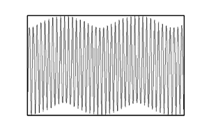
Figure 11. Variations of  $S = v _2 (x,0)$ normalized with its maximum at $y=0$ for $N _{\delta }=156$ (except plot (e) where $N _{\delta }=78)$ and selected $Pr$ values. The onset conditions in plots (a–f) are $(\alpha,\delta _{cr},Ra _{cr})$ = (4.39, 2.07, 3116.8), (4.95, 1.68, 3454.1), (4.31, 1.72, 2939.3), (4.91, 1.66, 3244.2), (4.3, 1.72, 2934.8), (9.01, 1.48, 7961.4) and the corresponding points are marked in figure 10 using letters identifying subfigures. Results are shown for (a) $Pr = 7$, (b) $Pr = 7$, (c) $Pr = 0.25$, (d) $Pr = 0.25$, (e) $Pr = 0.25$, ( f) $Pr = 0.04$.
Figure 10 illustrates possible states using  $N _{\delta }$. There is just a single band in the lock-in zone, but many distinct bands in the transition zone with similar characteristics for all $Pr$ values. These bands display certain inter-relations in the large- $\alpha$ limit, i.e. there are sets corresponding to a sequential doubling up of the system wavelength, i.e. $N _{\delta }=39, 78, 156$ and $N _{\delta }=117,234,468$, and then tripling up, i.e. $N _{\delta }=39,117$. Many other bands are possible, but their identification is compromised by the accuracy of the solution of the eigenvalue problem – while $\alpha$ is specified exactly, $\delta _{cr}$ is affected by the numerical error. The solution used spectral discretization, but computations relied on double precision arithmetic. The resolution can be improved by using quadruple precision or higher, but this was not possible in the present study.
Figure 11 provides data for characterization of flow patterns for  $N _{\delta } =156$ which are like those found for other $N _{\delta }$ values. The characterization is done using distributions of the $v _2$-velocity component along the mid-section of the slot at the onset and normalized with their maxima to focus on patterns only. Each cycle of $v _2$ signifies one pair of convection rolls. Figure 11(a, f) demonstrate the formation of ‘beating’ patterns for $\alpha$ slightly above the lock-in value for all $Pr$ values – the secondary motion consists of nearly identical rolls whose strength varies periodically. Figure 11(b–d) demonstrate the formation of ‘wavy’ patterns for $\alpha$ further away from $\alpha _{lc}$. Certain $x$-locations show a stronger upward movement while others show an opposite trend. A detailed look demonstrates roll pairs of different properties – at the beginning of a spatial cycle one roll is wider but with a less intense motion while the other is smaller with a more intense motion (see figure 12a) – their role is reversed after a half-cycle (figure 12b). The ‘beating’ pattern was not found for $Pr=0.25$ (no locked-in states) but ‘wavy’ patterns exhibit an abrupt change of the amplitude envelop (figure 11c,d). A completely different pattern is shown in figure 11(e) with every other roll being much narrower and much stronger. Only ‘beating’ patterns were found for $Pr=0.04$ (figure 11f). Analysis of the local wavenumber $\delta _{local}$ determined from the distance between two subsequent zeros of $v _2$ quantifies competition between the locked-in wavenumber $\delta _{cr}=\alpha /2$ and the RB wavenumber $\delta _{cr}=1.56$, with the ‘beating’ pattern strongly influenced by the lock-in and producing wide and flat maxima separated by narrow minima giving the appearance of a solitary phase modulation and forming a lattice parallel to the rolls (details not given). Solitons are known to mediate transition between the commensurate and incommensurate patterns (Lowe & Gollub Reference Lowe and Gollub1985; Mccoy et al. Reference Mccoy, Brunner, Pesch and Bodenschatz2008). For the ‘wavy’ pattern, these two effects are at par resulting in a rapid periodic adjustment of $\delta _{local}$ with its minima corresponding to locations where clockwise and anti-clockwise rotations have a similar intensity while its maxima correspond to locations with a preferred direction of rotation (details not shown).

Figure 12. The disturbance flow field corresponding to the ‘wavy’ pattern at the critical point ( $\alpha, \delta _{cr}, Ra _{cr}$) = (4.91, 3244.2, 1.66) for $Pr = 0.25$. The contour lines shown correspond to $\psi _2 (x,y)/\psi _{2,max} = 0, 0.01, 0.1, 0.5, 0.9$. Solid and dotted lines are used to identify rolls rotating in the opposite directions. This pattern belongs to the wavelength band $N _{\delta } = 156$.
Different types of responses are summarized in figure 13(a). Type A occurs for large  $Pr$ and is characterized by a nearly constant lock-in wavenumber $\alpha _{lc}$ and the lock-in critical Rayleigh number $Ra _{lc}$. Type B does not involve the lock-in. Type C includes the lock-in with rapid variations of both $\alpha _{lc}$ and $Ra _{lc}$. Type D involves two separate branches so the concepts of $\alpha _{lc}$ and $Ra _{lc}$ do not apply – one branch is associated with the lock-in and the other is unlocked. Variations of $\delta _{cr}$ as a function of $Pr$ for selected $\alpha$ values displayed in figure 13(b) illustrate peculiarity of the system response to variations of $Pr$, as there is a range of $\alpha$ where both small enough and large enough $Pr$ values produce locked-in states while the in-between $Pr$ values do not show the lock-in – this zone corresponds to a type B response identified in figure 13(a).

Figure 13. (a) Variations of the lock-in conditions, i.e. the lock-in heating wavenumber  $\alpha _{lc}$ and the critical Rayleigh number at the lock-in point $Ra_{lc}$, as functions of $Pr$. Triangles identify ends of the lock-in intervals. (b) Variations of the critical wavenumber $\delta _{cr}$ as a function of $Pr$ for selected $\alpha$ values. Diamonds identify conditions where locked-in and unlocked structures co-exist. Circles denote ends of the lock-in intervals. The RB limit of $\delta _{cr}=1.56$ is marked using a thin dotted line.
In order to determine the lowest heating intensity required to induce secondary convection assuming that one has an option to choose the type of fluid and the heating wavenumber, we construct figure 14 which depicts the required minimum Rayleigh number  $Ra _{cr,min}$ for each heating wavenumber denoted by $\alpha _{min}$ and the critical disturbance wavenumber by $\delta _{cr,min}$ as functions of $Pr$. The responses can also be qualitatively categorized as type A,B,C and D as the border lines shown in figure 14 correspond (qualitatively) to the borders identified in figure 13(a). In type A (fluids with $Pr>0.4$), intense heating is required (the $Ra _{cr,min}$ is higher) to induce the secondary convection, the heating wavenumber $\alpha _{min}$ monotonically decreases from 4.05 to an asymptotic value of 3.93, and $\alpha _{min}$ and $\delta _{cr,min}$ are locked-in. In type B, which occurs for $Pr$ between $\sim 0.4$ and $\sim 0.19$, intensity of the required heating and $\alpha _{min}$ gradually decrease with a decrease of $Pr$, and the lock-in does not occur. In type C, which occurs for $\sim 0.08 < Pr < \sim 0.19$, intensity of the required heating rapidly decreases with a decrease of $Pr$,
$Pr$,  $\alpha _{min}$ and $\delta _{cr,min}$ become locked-in with both wavenumbers slightly increasing with a decrease of $Pr$. In type D, which occurs for fluids with $Pr<0.04$, weak heating (e.g. as low as $Ra _{cr,min}=314.3$ for $Pr=0.01$) is sufficient to induce the secondary convection, the lock-in occurs and both $\alpha _{min}$ and $\delta _{cr,min}$ remain nearly constant at 4.02 and 2.01, respectively.

Figure 14. Variations of the minimum Rayleigh number  $Ra _{cr,min}$ (solid line) required to induce secondary convection, the corresponding heating wavenumber $\alpha _{min}$ (upper dashed line) and the critical disturbance wavenumber $\delta _{cr,min}$ (lower dashed line) as functions of $Pr$.
$Pr$.
4. Summary
Multiple forms of response of a fluid layer exposed to spatially periodic heating were identified. The system is charaterized by two wavenumbers: one characterizes the pattern of externally imposed heating ( $\alpha$), while the other is determined by the instability processes ( $\delta$). The system response is driven by a competition between two instability mechanisms, i.e. the spatial parametric resonance and the RB mechanism. The spatial parametric-resonance-dominated response exhibits the characteristic lock-in between the primary and secondary convection. Both states are unlocked when the RB instability dominates, and the structure of the resulting convection is very similar to RB convection. Convection in the transition zone between the lock-in states and the RB-like states creates a spectrum of commensurate and incommensurate states with only the former being accessible to numerical solutions due to limitations of computer accuracy. These states can be organized into discrete bands of wavelengths with the resulting movement exhibiting ‘wavy’ and ‘beating’ patterns. Since the bands reported in this paper are constructed by retaining two digits from a four-digits-accurate computed $\delta _{cr}$, other patterns may emerge if the bands are constructed using more accurate data.
The first mechanism referred to above, i.e. spatial parametric resonance, dominates if the spatial modulation of the primary state is sufficiently strong while the second one, the RB instability, dominates for weak spatial modulations. The strength of modulation decreases with an increase of  $Pr$ and an increase of $\alpha$. An increase of $Ra$ increases the intensity of the fluid motion but it increases modulation only for $\alpha <\sim 10$ and has no effect on the modulation for $\alpha >10$. The possible responses for different fluids can be divided into four types. In type A, which occurs for fluids with $Pr > \sim 0.4$, the spatial parametric resonance dominates for $\alpha <~4.5$ resulting in a lock-in of the critical wavenumber $\delta _{cr}$ with the heating wavenumber by a sub-harmonic relation, e.g. $\delta _{cr}= \alpha /2$. For larger values of $\alpha$ (e.g. $\alpha >10$), a convection boundary layer forms near the heated wall producing a uniform vertical temperature gradient above it leading to the dominance of the RB mechanism and elimination of any relation between the primary and secondary flow patterns. In the in-between zone of $\alpha$, where neither mechanism dominates, an interplay of both mechanisms creates conditions where a small change in $\alpha$ results in a major change in the flow pattern, thereby providing a wealth of possible system responses. Morphing between different convection patterns may occur in response to minor changes of the heating pattern. In type B, which occurs for $Pr$ between ${\sim }0.4$ and ${\sim }0.19$, the RB mechanism dominates and the lock-in between the instability and the heating patterns does not occur. In type C, which occurs for ${\sim }0.08 < Pr<\sim 0.19$, the stronger spatial modulation causes a pattern of instability to lock-in with the heating pattern for $\alpha$ values up to $\alpha ={\sim }7$. The RB effect prevails for $\alpha >10$, and in the in-between zone of $\alpha$ ( $\alpha =7 \sim 10$) a wealth of possible patterns occurs, similarly as in type A. It is found that for type C, the change of the lock-in wavenumber $\alpha _{lc}$ and the change of the lock-in Rayleigh number $Ra _{lc}$ occur rapidly with the change of $Pr$, whereas for type A, the changes of $\alpha _{lc}$ and $Ra _{lc}$ are very gradual ( $\alpha _{lc}$ vs $Pr$ and $Ra _{lc}$ vs $Pr$ curves are almost flat). In type D, which occurs for $Pr < 0.08$, two separate critical instability branches have been identified. Branch 1 describes the critical conditions for parametric resonance and corresponds to disturbances whose structure is locked-in with the heating pattern. Branch 2 describes the critical conditions for the RB-dominated instability and corresponds to disturbances whose patterns have no relation with the heating patterns. The critical conditions when both types of patterns co-exist have been identified. Among the four types of responses outlined above, it is observed that the locked-in pattern (branch 1) of type D requires the weakest heating (e.g. as low as $Ra _{cr,min} = 314.3$ for $Pr=0.01$ at $\alpha =4.02$) to create secondary motions.
Similar responses are expected to occur when heating is applied to the upper wall. Heating of both walls introduces a phase difference that may qualitatively change the system response. The addition of weak forced convection is not expected to produce major changes.
Funding
This work has been carried out with the support from NSERC of Canada.
Declaration of interests
The authors report no conflict of interest.
Appendix A. Primary convection formulation: method of solution
This appendix illustrates the method of solution of the governing equations (2.4) describing the primary convection presented in § 2.
We start the solution of the governing equations (2.4) by introducing the streamfunction  $\psi _1 (x,y)$ defined in the usual manner as $u _1 = {\partial \psi _1} / {\partial y}$, $v _1 = -{\partial \psi _1} / {\partial x}$, and eliminating the pressure field from the momentum equations resulting in
 \begin{gather} \nabla^4 {\psi _1} - Ra \frac{\partial \theta _1}{\partial x} - Ra Pr ^{{-}1} \frac{\partial \theta _c}{\partial x} = N _1, \end{gather}
 \begin{gather} \nabla^2 \theta _1 = N _2, \end{gather}
where terms involving products and nonlinearities are expressed as
 $$\begin{gather} N_1=\frac{{\partial }}{\partial y} \left ( \frac{\partial }{\partial x} \langle u_1 u_1 \rangle + \frac{\partial }{\partial y} \langle u_1 v_1 \rangle \right ) - \frac{{\partial }}{\partial x} \left ( \frac{\partial }{\partial x} \langle u_1 v_1 \rangle + \frac{\partial }{\partial y} \langle v_1 v_1 \rangle \right ), \end{gather}$$
 $$\begin{gather}N_2=Pr \left ( \frac{{\partial }}{\partial x} \langle u_1 \theta_1 \rangle + \frac{{\partial }}{\partial y} \langle v_1 \theta_1 \rangle \right ) +\frac{{\partial }}{\partial x} \langle u_1 \theta_c \rangle + \frac{{\partial }}{\partial y} \langle v_1 \theta_c \rangle. \end{gather}$$
We assume the solution in the form of Fourier expansions,
 \begin{gather} [ \psi _1, \theta _1 ] (x,y) = \sum _{n={-}\infty} ^{n ={+}\infty} [ \varphi _{1} ^{(n)}, \phi _{1} ^{(n)} ] {\rm e}^{{\rm i}\, n \alpha x}, \end{gather}
 \begin{gather} \left [ u _1, v _1 \right ] (x,y) = \sum _{n={-}\infty} ^{n ={+}\infty} [ u _{1} ^{(n)}, v _{1} ^{(n)}] {\rm e}^{{\rm i}\, n \alpha x}, \end{gather}
where  $\varphi _{1} ^{n} = \varphi _{1} ^{(-n) *}$, $\phi _{1} ^{n} = \phi _{1} ^{(-n) *}$, $u _{1} ^{n} = u _{1} ^{(-n) *}$ and $v _{1} ^{n} = v _{1} ^{(-n) *}$ represent the reality conditions and stars denote complex conjugates, $u ^{(n)} = D \varphi _{1} ^{(n)}$, $v ^{(n)} = {\rm i}\, n \alpha \varphi _{1} ^{(n)}$ and $D = {{\partial }}/{\partial y}$. The nonlinear and product terms are also expressed in terms of Fourier expansions in the form
 \begin{gather} \left [ \langle u_1 u_1 \rangle, \langle u_1 v_1 \rangle, \langle v_1 v_1 \rangle \right ] (x,y) = \sum _{n={-}\infty} ^{n ={+}\infty} [ \langle u_1 u_1 \rangle^{(n)}, \langle u_1 v_1 \rangle^{(n)}, \langle v_1 v_1 \rangle^{(n)} ] {\rm e}^{{\rm i} n \alpha x}, \end{gather}
 \begin{gather} \left [ \langle u_1 \theta_1 \rangle,\!\langle v_1 \theta_1 \rangle, \langle u_1 \theta_c \rangle, \langle v_1 \theta_c \rangle \right ] (x,y) \,{=} \sum _{n={-}\infty} ^{n ={+}\infty} [ \langle u_1 \theta_1 \rangle^{(n)}, \langle v_1 \theta_1 \rangle^{(n)},\!\langle u_1 \theta_c \rangle^{(n)},\!\langle v_1 \theta_c \rangle^{(n)} ] {\rm e}^{{\rm i} n \alpha x}. \end{gather}
Substitution of (A4) into (A1) and separation of Fourier components results in the following system of ordinary differential equations for the modal functions:
 \begin{gather} D _n ^2 {\varphi _1} ^{(n)} - {\rm i}\,n \alpha Ra \phi _1 ^{(n)} = {\rm i}\,n \alpha Ra \theta _c ^{(n)} + N _1 ^{(n)}, \end{gather}
 \begin{gather} D _n {\phi _1} ^{(n)} = N _2 ^{(n)}. \end{gather}
Here  $D={\rm d}/{{\rm d} y}$, $D^2 = {\rm d}^2/{{\rm d} y}^2$, $D_n=D^2 - n^2 \alpha ^2$, $D ^2 _n=D _n(D_n)$, $N_1^{(n)} = {\rm i}\,n \alpha D \langle u_1 u_1 \rangle ^{(n)} + D^2 \langle u_1 v_1 \rangle ^{(n)} + {\rm i}\,n^2 \alpha ^2 \langle u_1 v_1 \rangle ^{(n)} - {\rm i}\,n \alpha D \langle v_1 v_1 \rangle ^{(n)}$, $N_2^{(n)} = Pr ( {\rm i}\,n \alpha \langle u_1 \theta _1 \rangle ^{(n)} + D \langle v_1 \theta _1 \rangle ^{(n)} ) + {\rm i}\,n \alpha \langle u_1 \theta _c \rangle ^{(n)} + D \langle v_1 \theta _c \rangle ^{(n)}.$ The required boundary conditions have the form
 \begin{equation} {\varphi _1} ^{(n)} ({\pm} 1) = 0, D{\varphi _1}^{(n)} ({\pm} 1) = 0, {\phi _1}^{(n)} ({\pm} 1) = 0 \quad{\rm for} -\infty < n<{+}\infty. \end{equation}
In the system (A5) the unknown linear terms have been placed on the left-hand side, and the nonlinear and product terms have been placed on the right-hand side. For the purpose of numerical solution, expansions (A4) have been truncated after  $N_M$ Fourier modes. The discretization method uses the Chebyshev collocation technique based on the Gauss–Chebyshev–Lobatto points (Canuto et al. Reference Canuto, Hussaini, Quarteroni and Zang1996). The resulting nonlinear algebraic system was solved using an iterative technique combined with under-relaxation.
Appendix B. Secondary convection formulation: method of solution
This appendix illustrates the solution procedure of the governing equations describing the secondary convection presented in § 3.
Similar to the primary convection, we introduce the disturbance streamfunction  $\psi _2 (x,y)$ defined as $u _2 = {\partial \psi _2} / {\partial y}$, $v _2 = -{\partial \psi _2} / {\partial x}$, and eliminate the pressure field $p_2$ from the disturbance momentum equations.
The forms of disturbances described by (3.3)–(3.4) are applied to  $\psi _2$ and $\theta _2$ as
 \begin{equation} {[} \boldsymbol{\psi _2}, \theta _2 ](x,y,t) = \sum _{m={-}\infty} ^{m={+}\infty} [\boldsymbol{\varPsi _2 ^{(m)}}, \varTheta _2 ^{(m)}] (y) {\rm e}^{{\rm i}\, m \alpha x } {\rm e}^{{\rm i} (\delta x -\sigma t)} +{\rm c.c.} \end{equation}
Substitution of (B1) into the disturbance equations (3.2) and separation of Fourier components result, after a rather tedious algebra, in a system of linear homogeneous ordinary differential equations in the form
 $$\begin{align} A^{(m)} \varPsi _2
^{(m)} -{\rm i}\, t_m Ra \varTheta _2 ^{(m)} &= {\rm i}\,
\sum _{n={-}\infty} ^{n={+}\infty} [t_n D \varphi _1
^{(m-n)} H^{(n)} \varPsi _2 ^{(n)} +(m-n) \alpha I^{(m-n)}
\varphi _1 ^{(m-n)} D \varPsi _2 ^{(n)} \nonumber\\
&\quad -(m-n)\alpha \varphi _1 ^{(m-n)}H^{(n)}D
\varPsi _2 ^{(m)} -t_n I ^{(m-n)} D\varphi _1 ^{(m-n)}
\varPsi _2 ^{(n)}],\end{align}$$
$$\begin{align} A^{(m)} \varPsi _2
^{(m)} -{\rm i}\, t_m Ra \varTheta _2 ^{(m)} &= {\rm i}\,
\sum _{n={-}\infty} ^{n={+}\infty} [t_n D \varphi _1
^{(m-n)} H^{(n)} \varPsi _2 ^{(n)} +(m-n) \alpha I^{(m-n)}
\varphi _1 ^{(m-n)} D \varPsi _2 ^{(n)} \nonumber\\
&\quad -(m-n)\alpha \varphi _1 ^{(m-n)}H^{(n)}D
\varPsi _2 ^{(m)} -t_n I ^{(m-n)} D\varphi _1 ^{(m-n)}
\varPsi _2 ^{(n)}],\end{align}$$
 $$\begin{align} C^{(m)} \varTheta _2
^{(m)} &= {\rm i}\, Pr \sum _{n={-}\infty} ^{n={+}\infty}
[t_n D \varphi _1 ^{(m-n)} \varTheta _2 ^{(n)} +(m-n)
\alpha \vartheta _1 ^{(m-n)} D \varPsi _2 ^{(n)}\nonumber\\ &\quad -(m-n)\alpha \varphi _1
^{(m-n)} D \varTheta _2 ^{(m)} - t_n D \vartheta _1
^{(m-n)} \varPsi _2 ^{(n)}],
\end{align}$$
$$\begin{align} C^{(m)} \varTheta _2
^{(m)} &= {\rm i}\, Pr \sum _{n={-}\infty} ^{n={+}\infty}
[t_n D \varphi _1 ^{(m-n)} \varTheta _2 ^{(n)} +(m-n)
\alpha \vartheta _1 ^{(m-n)} D \varPsi _2 ^{(n)}\nonumber\\ &\quad -(m-n)\alpha \varphi _1
^{(m-n)} D \varTheta _2 ^{(m)} - t_n D \vartheta _1
^{(m-n)} \varPsi _2 ^{(n)}],
\end{align}$$
where
 \begin{equation} \left. \begin{gathered} A^{(m)} = (D^2-t_m^2)^2 + {\rm i}\, \sigma (D^2 - t_m^2), \\ C^{(m)} = D^2-t_m^2 + {\rm i}\, Pr \sigma ,\\ \vartheta _1 ^{(m)} = Pr^{{-}1} \theta _c ^{(m)}+\phi _1 ^{(m)}, \\ I^{(m-n)} = D^2-(m-n)^2 \alpha ^2, \\ H^{(n)} = D^2-t_n^2 ,\\ t_m = \delta+ m \alpha,\\ t_n= \delta+ n \alpha. \end{gathered} \right\} \end{equation}
The boundary conditions take the form
 \begin{equation} \varPsi _2 ^{(m)}({\pm} 1)=0, \quad D \varPsi _2 ^{(m)}({\pm} 1)=0, \quad \varTheta _2 ^{(m)}({\pm} 1)=0 \quad {\rm for}\ -\infty < m<{+}\infty. \end{equation}
Equations (B2) are truncated after  $N_M$ modes and are discretized with spectral accuracy using the Chebyshev collocation method with $N_T$ collocation points (Canuto et al. Reference Canuto, Hussaini, Quarteroni and Zang1996). The resulting eigenvalue problem is solved by the ‘inverse iteration’ technique as described in Saad (Reference Saad2011).


 Open access