


Introduction
Receipt of solar radiation is one of the fundamental controls on glacier and ice-sheet mass balance, accounting for up to 99% of the energy available for melt at a glacier surface (Reference ArendtArendt, 1999), although figures of ∼75% are perhaps more usual (e.g. Reference Greuell and SmeetsGreuell and Smeets, 2001; Reference Klok and OerlemansKlok and Oerlemans, 2002). In order to accurately calculate solar radiation receipts, one of the fundamental requirements of glacier mass- and energy-balance models is an accurate digital elevation model (DEM) of the glacier and, in the case of valley glaciers, the surrounding topography, as topography (together with the solar geometry and surface albedo) is the fundamental control on the receipt of solar energy. Shading by the surrounding terrain, as well as slope and aspect variations over the glacier surface itself, will affect the amount of direct solar radiation received; ‘overlook’ of the glacier surface by surrounding high relief will affect the amount of diffuse solar radiation and incoming longwave radiation by obscuring part of the sky. Surrounding high topography will also reflect direct solar radiation and emit longwave radiation which may be received elsewhere within the catchment.
The spatial resolution of the DEMs used to date in distributed surface energy-balance models of glaciers has typically been several tens of metres (e.g. Reference Arnold, Willis, Sharp, Richards and LawsonArnold and others, 1996: 20 m; Reference Klok and OerlemansKlok and Oerlemans, 2002: 25 m; Reference Hock and NoetzliHock and Noetzli, 1997; Reference Hock and HolmgrenHock and Holmgren, 2005: 30 m). The choice of resolution in these studies seems to have been largely pragmatic; it gives a useful amount of small-scale detail, but as the DEMs have typically been based on either digitized contour maps, or sparse, interpolated survey data, such a resolution does not try to bring in too much (effectively spurious) detail by interpolating such data to very fine spatial resolutions. Many of these studies have emphasized the importance of topography in controlling direct solar radiation receipts (both spatial distributions and total amounts), and hence the overall energy balance and mass balance of glaciated surfaces. Reference Arnold, Willis, Sharp, Richards and LawsonArnold and others (1996) show that including the effects of shading reduces calculated direct solar radiation receipts by 5%, and including slope and aspect reduces calculated radiation by 15% for Haut Glacier d’Arolla, Switzerland, in comparison with calculations which neglect these factors. In a similar set of experiments, Reference Klok and OerlemansKlok and Oerlemans (2002) show that shading reduces radiation receipts by 10%, and slope and aspect by 9% for Morteratschgletscher, Switzerland, and Reference Arnold, Rees, Hodson and KohlerArnold and others (2006b) show that shading reduces radiation receipts by 6%, but slope and aspect by only 0.3%, for midre Lovénbreen, Svalbard. They, however, suggest that this small figure is due to the very high latitude (∼79° N) of this glacier, meaning that the sun shines from all directions during the 4 months of 24 hour daylight, effectively cancelling the impact of slope and aspect on solar radiation receipts.
Calculated values of distributed solar radiation receipts have also been used to improve the effectiveness of temperature-index models of glacier melt (e.g. Reference Cazorzi and Dalla FontanaCazorzi and Dalla Fontana, 1996; Reference HockHock, 1999; Reference Pellicciotti, Brock, Strasser, Burlando, Funk and CorripioPelliccioti and others, 2005; Reference SchulerSchuler and others, 2005) in areas without the detailed meteorological input data needed to drive energy-balance models.
Reference Chasmer, Hopkinson, Hardy and FrankensteinChasmer and Hopkinson (2001) have used lidar data interpolated to 2.5 and 25 m spatial resolution to assess the impacts of DEM resolution on instantaneous radiation loading for a mid-latitude glacier (Peyto Glacier, Canadian Rocky Mountains) for two periods in winter and summer; they found that mean catchment radiation was overestimated, yet maximum radiation was underestimated, when using the coarse-resolution DEM, especially at low solar angles.
Given the importance of solar radiation receipts for glacier surface energy balance and mass balance, in this paper we extend this analysis to investigate the impact of DEM scale on yearly totals of potential direct-beam solar radiation receipt, the total potential duration of direct-beam solar radiation, and the mean intensity of potential direct-beam solar radiation. We apply this analysis to a high-latitude Arctic glacier, midre Lovénbreen, northwest Svalbard (Fig. 1). Midre Lovénbreen is a small, predominantly north-facing glacier on the northwest coast of Spitsbergen, Svalbard (Fig. 1). The glacier has an area of about 6 km2, with an altitude range of 50–550 m a.s.l. and a maximum thickness of around 180 m (Reference BjörnssonBjörnsson and others, 1996). We then also investigate the impact of DEM resolution on the summer-season energy balance of midre Lovénbreen using a distributed surface energy-balance model (Reference Arnold, Rees, Hodson and KohlerArnold and others 2006b).
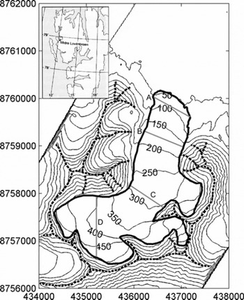
Fig. 1. Location map for midre Lovénbreen, with contours based on a 20 m spatial resolution DEM derived from airborne lidar data collected during 2005. Eastings and northings are Universal Transverse Mercator (UTM) coordinates, based on the World Geodetic System 1984 (WGS84) datum. The UTM zone is 33X. Heavy solid curve shows the glacier margin. Heavy dashed curve shows cells assigned the maximum measured height in the ‘ridge DEM’; grey lines show transect locations.
Data and Methodology
Primary data requirements for the model are an appropriately scaled DEM of the glacier surface and surrounding topography, and solar altitude and azimuth data at an appropriate temporal resolution for the length of the model run.
Topographic data
The DEMs used in this study were derived from airborne lidar data collected during the summer of 2005. The raw data were collected at a variable spatial resolution (depending on the elevation of the aircraft above the ground) of 0.7–1.5 m. A more detailed discussion of similar lidar data collected in 2003 is given by Reference Arnold, Rees, Devereux and AmableArnold and others (2006a); we use the same methods here to analyse and evaluate the 2005 data. The root-mean-square error (RMSE) in the lidar height measurements varies from <0.05 m on the upper glacier to <0.1 m on the lower glacier; the RMSE in the horizontal positions of the measurements is <0.025 m. For this study, DEMs were produced from these data at spatial resolutions of 2.5, 5, 10, 20, 50, 100, 200, 400, 1000 and 2000 m, firstly by taking the mean of all measured lidar elevations within each appropriately sized DEM gridcell as the height of that cell (hereafter referred to as the ‘mean DEM’). In the light of the results of solar radiation calculations, two more sets of DEMs were constructed. In the first of these (hereafter referred to as the ‘ridge DEM’), any cells in the mean DEM which were higher than any five (or more) of the surrounding eight cells were assumed to be local topographic high points, and were assigned the maximum measured lidar point height from the set of measurements within such a cell, rather than the mean value; other cells were unchanged from the mean DEM. This effectively increased the height of the ridges surrounding the catchment, especially in the coarser-resolution DEMs, but had little or no impact on the height of the glacier itself, where topographic variation was far smaller. As an example, cells allocated the maximum measured height for the 20 m DEM are shown in Figure 1; the effectiveness of this simple algorithm at detecting high, linear features is clear. We produced a third set of DEMs in which all cells were assigned the maximum measured height from the set of lidar height measurements located in each cell (the ‘maximum DEM’). In addition to these DEMs, we also created a planar DEM for reference purposes, with the same mean height as the glaciated cells in the 2.5 m mean DEM.
In order to check whether the impact of DEM resolution depended on the overall aspect of the glacier, we also conducted runs at the various resolutions with the mean DEM rotated by 90°, 180° and 270°. We also performed some calculations with DEMs with cell centres offset by 2.5 m.
Cell slope and aspect were calculated using the second-order finite-difference method of Reference Zevenbergen and ThorneZevenbergen and Thorne (1987). Although many different slope and aspect estimators exist, this algorithm was ranked first in a study of actual and artificial DEMs by Reference JonesJones (1998). However, we also ran the model using the third-order finite-difference operator of Reference HornHorn (1981), which is used by the ArcView ‘slope’ command. This change made <∼0.005% difference to the total calculated yearly potential direct solar radiation over the glacier at the finest resolutions; at the coarsest resolution, this algorithm changed the total by ∼0.5% for the mean DEMs.
Solar radiation calculations
The theoretical potential instantaneous direct-beam (clear-sky) solar radiation, I (W m −2), is calculated as a function of the top-of-atmosphere (TOA) solar radiation, an assumed atmospheric transmissivity, and solar and surface geometry, following Reference OkeOke (1987):
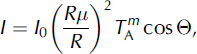
where I 0 is the solar constant (13 68 W m−2; Reference Fröhlich, McBean and HantelFröhlich 1993), R is the instantaneous Earth–Sun distance at the time period in question (m) and R μ is the mean Earth–Sun distance (1.496 × 10¹¹ m). T A is the mean atmospheric clear-sky transmissivity and m is the optical air mass. T A varies between 0.9 and 0.6, with atypical value of 0.84 (Reference CampbellCampbell, 1977, cited by Reference OkeOke, 1987). Reference HockHock (1999) uses a value of 0.75; in this study, we use a value of 0.8262, derived from measured direct-beam solar radiation at a synoptic weather station maintained by the Alfred Wegener Institute (AWI) at Ny-Ålesund, approximately 5 km from the glacier (Reference König-Langlo, Marx, Lautenschlager and ReinkeKönig-Langlo and Marx, 1997). Our fitting procedure is discussed below.
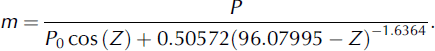
The simplest algorithm for calculating m is simply P/(P 0sec(Z)), where P is the atmospheric pressure, P 0 is the mean sea-level atmospheric pressure (101.3 kPa) and Z is the solar zenith angle (°). However, this relationship becomes increasingly inaccurate for Z>80° (Reference OkeOke, 1987), tending to infinity at Z = 90° whereas the true value tends to ∼38 (e.g. Reference Kasten and YoungKasten and Young, 1989). Given that the sun is often quite close to the horizon in the High Arctic, we therefore use the formula proposed by Reference Kasten and YoungKasten and Young (1989) for air mass, corrected for atmospheric pressure variations:
P varies only with altitude in the model; we use a lapse rate of 0.011 kPa m−1 (NASA/NOAA, 1976). O in Equation (1) is the angle of incidence between the normal to the DEM cell and the solar beam. This is calculated from the solar zenith angle and solar azimuth (A sun), and surface slope (β) and aspect (A slope) (Reference Garnier and OhmuraGarnier and Ohmura, 1968):
Solar geometry is calculated using the algorithms of Reference MichalskyMichalsky (1988), which have a stated accuracy of 0.01° between 1950 and 2050. Although more accurate algorithms exist (e.g. Reference Reda and AndreasReda and Andreas, 2004), the added complexity of implementing such algorithms here is not justified, in that the errors produced by a change in the calculated solar position of 0.01° are comparable with those associated with the RMSE in the lidar heights and horizontal position data.
Shading of the glacier surface by the surrounding topography is calculated using the method of Reference Arnold, Willis, Sharp, Richards and LawsonArnold and others (1996); as we consider only the direct solar radiation, if a DEM cell is shaded, I is set to zero. For time periods in which the sun is below the horizon, I is also set to zero. In addition to this, I is set to zero for any cells for which cos Θ is <0, as such cells are self-shaded; the sun is below a local horizon created by the edge of the cell itself.
Total annual potential direct-beam solar radiation values (I tot; MJ m−2) across the glacier are calculated by applying Equation (1) at a 15 min resolution for one calendar year (we use 2003) and summing the results. We also calculate the total duration of potential direct-beam solar radiation (I dur; h) (i.e. the total time for which the sun is above the horizon and the cell in question is not shaded) for each DEM cell. From these values we then also calculate the mean intensity of potential direct-beam solar radiation for each DEM cell (Iint; W m−2); this is the quotient of Itot and Idur.
We also calculate the sky-view factor, fs, for each cell in each DEM cell in question using the relationship:
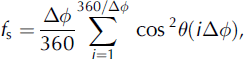
where θ(φ) is the local horizon angle at a given azimuth, φ. Following Reference Arnold, Rees, Hodson and KohlerArnold and others (2006b), Δφ is set to 12°. This type of relationship (a sum of horizon angles at discrete azimuth intervals) has been used in other studies (e.g. Reference Greuell, Knap and SmeetsGreuell and others, 1997; Reference Müller and SchererMüller and Scherer, 2005). It includes the effect of the local cell slope because at high slope angles, the horizon in particular directions can be formed by the edge of the cell itself.
Tuning and validation
The key unknown in the solar radiation calculations is the value of φ A, the mean atmospheric clear-sky transmissivity. We have derived a best-fit value for this study by using measured direct-beam solar radiation data and cloud base height from the AWI meteorological data for 1997–2000. We calculate an atmospheric transmissivity value by dividing measured direct-beam solar radiation by the model-derived TOA radiation (i.e. I 0 (Rμ = R)2 from Equation (1)). The measured direct-beam solar radiation is affected by cloud and other atmospheric effects, as the model considers the potential direct-beam solar radiation under clear-sky conditions. We eliminate the effect of cloud as far as possible by only using data for times when the cloud-base is measured as >30000 m (the upper limit for measured values from the laser ceilograph used to make the cloud-based height measurements). This yields a dataset of 780 cloud-free observations for the 4 years used for calibration.
This calculated transmissivity value includes the effect of changing solar zenith angle (i.e. the value is equal to ![]() ). We then use calculated solar zenith angle data to derive a best-fit value for T
A with m calculated from Equation (2) at the times in question, and taking the station pressure as the standard atmospheric pressure. For the best-fit value of m = 0.8262, we obtain an R
2 value of 0.66 for 780 data points, significant at P < 0.0001.
). We then use calculated solar zenith angle data to derive a best-fit value for T
A with m calculated from Equation (2) at the times in question, and taking the station pressure as the standard atmospheric pressure. For the best-fit value of m = 0.8262, we obtain an R
2 value of 0.66 for 780 data points, significant at P < 0.0001.
We then validate this model by comparing the modelled potential direct-beam radiation against measured direct-beam solar radiation from the AWI meteorological station for the period 2001–03, again using only those time periods when the cloud base is measured as ≥30000 m.
In addition, during the 2003 and 2005 lidar campaigns, we obtained very high-resolution radiometric (Airborne Thematic Mapper (ATM)) images of the glacier. As the flights were made in clear-sky conditions, the extent of shading of the glacier surface is clearly visible, and we have compared the extent of shading in a georeferenced 2 m spatial resolution image collected on 9 August 2003 with that predicted by the shading algorithm, based on a 2 m spatial resolution DEM.
Impact on overall mass and energy balance
In order to assess the impact of DEM resolution on the glacier summer energy balance, we carried out a set of runs using the full energy-balance model of Reference Arnold, Rees, Hodson and KohlerArnold and others (2006b). This calculates the sensible and latent turbulent heat fluxes, the net solar and longwave radiative fluxes, and includes a scheme to calculate the temperature of the glacier surface. Calculated snow-depth changes are tracked during the melt season; changing snow depth is the primary control on temporal variations in albedo during the model runs.
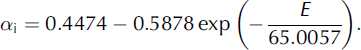
The surface albedo (α s) is calculated using a simple empirical scheme based on measurements made in summer 2000 using the modelled snow depth (D SWE; mw.e.) and the albedo of the underlying surface (α i):

α i is modelled with a simple empirical relationship with elevation (E; ma.s.l.) again based on data collected in summer 2000:
Rather than use meteorological data measured on the glacier, as done by Reference Arnold, Rees, Hodson and KohlerArnold and others (2006b), we use the data for 2001–03 measured at the AWI meteorological station. These data include the direct and diffuse components for solar radiation. Topographic correction of the direct-beam component for each DEM cell is made using the solar and surface geometry calculations and the shading algorithm discussed above. For shaded areas, only the diffuse component is used in the energy-balance calculations, modified by the calculated sky-view factor.
We use simple best-fit cubic polynomial interpolations of the measured winter snow depths against elevation for 2001–03 from mass-balance measurements made by the Norsk Polarinstitutt (J. Kohler, unpublished data) to initialize the model at the start of each melt season. Over the elevation range of the glacier, these curves do not produce extreme high or low values. All other parameters are taken from Reference Arnold, Rees, Hodson and KohlerArnold and others (2006b). The model is applied for the period 25 April–12 September in each year. These dates were chosen as they broadly correspond to the dates when the Norsk Polarinstitutt summer and winter balance measurements are made (Kohler, unpublished data), and because the focus of this study is on the impact of DEM resolution on solar radiation receipts in particular, so the energy balance during winter does not concern us here.
Results and Discussion
Validation
Figure 2 shows measured and modelled potential direct-beam radiation for the calibration period 2001–03. This yields an R 2 value of 0.97 for the 1549 observations with cloud base ≥30000 m during the test period, significant at P .0001. The scatter of points above the main trend line, where modelled radiation exceeds observed radiation, is most simply explained by the presence of patchy rather than continuous cloud. In such conditions it would be quite possible for the cloud-base measurement to show clear conditions but for the measured direct-beam radiation to be affected by cloud elsewhere in the sky. This would lead to the model relationship (which assumes clear skies) over-predicting the radiation for that time. The ‘reverse’ effect is not observed; no points lay some distance below the main cluster of points.
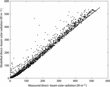
Fig. 2. Measured direct-beam solar radiation for clear-sky periods in 2001–03 plotted against modelled direct-beam solar radiation for the same time periods. Values are 5 min averages of the instantaneous flux. The 1 :1 line is also shown.
The slope of the regression line is 1.06, implying the model relationship has a small tendency to under-predict low values and over-predict high values; the season-long totals are within 2%, however, which, given that the observed total will include periods when the direct-beam measurements are affected by cloud, is a very good match. Visual comparison of the ATM image with shading calculated by the model showed an almost perfect match.
Impact of DEM resolution on solar radiation receipts
Figure 3 shows the spatial distribution of annual total potential direct-beam solar radiation (I tot) over the glacier for the (a) 5 m, (b) 20 m, (c) 50 m and (d) 200 m resolution mean DEMs. Three of the four distributions show an obvious resemblance. The exception is the 200 m DEM, which shows serious deficiencies in many areas. At coarser resolutions, the pattern degrades further: at 2000 m resolution, the glaciated part of the catchment is represented by only one DEM cell, so all spatial detail is lost. However, at finer resolutions, there are differences in the detail. The 5 m DEM, in particular, shows a ‘fuzziness’ in the contour lines which reflects an increase in the very small-scale spatial variation in I tot. This is especially true on the main tongue of the glacier, and towards the snout. At 2.5 m resolution, this effect is even more marked, and when plotted at the same scale, the contours themselves obscure much of the spatial detail. Another subtle difference is that there is a trend towards an increase in I tot as the DEM resolution coarsens; the most obvious manifestation of this is the increase in size of the areas of highest I tot, especially on the middle and upper parts of the glacier. This is particularly marked for the 200 m DEM.
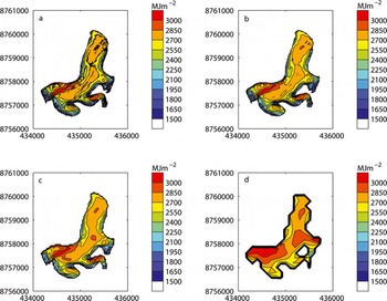
Fig. 3. Yearly total potential direct-beam solar radiation (I tot; MJ m−2) at different DEM resolutions: (a) 5 m; (b) 20 m; (c) 50 m; (d) 200 m. Eastings and northings are UTM coordinates, UTM zone 33X.
These differences are borne out in Figure 4, which shows I tot at four transects across the glacier (Fig. 1) for DEM resolutions from 2.5 to 200 m. These show a decrease in the ‘detail’ as resolution coarsens, but there is also a systematic increase in the values at any given location across the glacier as DEM resolution coarsens, manifest as an ‘offset’ between the lines for the various DEM resolutions (except for the central parts of the lowest transect, A). This increase becomes larger at the coarsest resolutions; there is also a tendency for the offset to be larger towards the margins of the glacier, with a smaller offset nearer the centre line.
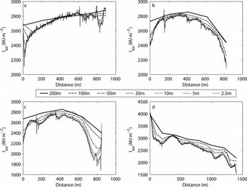
Fig. 4. Yearly total potential direct-beam solar radiation (I tot; MJ m−2) for the four transect locations shown in Figure 1 at different DEM resolutions, based on the ‘mean DEMs’.
A similar pattern occurs for the total duration of potential direct-beam solar radiation (I dur) (Fig. 5). Again, except for transect A (the reasons for this are discussed below), there is an increase in I dur at any given location at coarser DEM resolutions. The overall shape of the distributions of both I tot and I dur is similar for transects A–C. However, I dur for transect D (Fig. 5d) shows a different pattern than I tot (Fig. 4d) because of the change in orientation of this transect (north–south) relative to the others (which broadly run northwest–southeast). I tot (Fig. 4d) decreases with distance partly due to topographic shading, but also because of the overall steepening of the glacier surface towards the south, coupled with the northerly aspect of the surface. This change in steepness, however, does not affect I dur, which therefore has a flatter distribution along the transect, until around 1100 m distance when the duration drops markedly due to shading. Again, however, the increase in I dur at coarser resolutions is apparent.
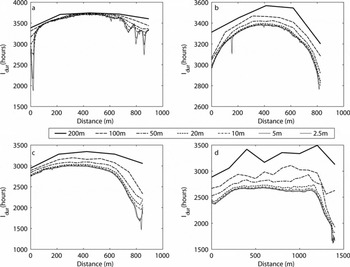
Fig. 5. Yearly total potential duration of direct-beam solar radiation (Idur; hours) for the four transect locations shown in Figure 1 at different DEM resolutions, based on the mean DEMs.
These differences can be summarized by calculating the whole-glacier spatial mean (defined as the sum of the values for each gridcell, divided by the number of cells) of I tot (Fig. 6a, solid curve). This shows a clear dependency on the DEM resolution, with the spatial mean I tot increasing as DEM resolution coarsens. The relationship between resolution and spatial mean I tot is non-linear, however, having a broadly sigmoid shape. At resolutions finer than ∼20 m, the impact of resolution is not particularly marked, but the rate of change of the spatial mean gradually increases as resolution coarsens. The reduction in the impact at the finest resolutions suggests that the calculations are approaching an asymptotic value, and using resolutions finer than perhaps 1–2 m will not improve distributed solar radiation calculations; it could be said that finer resolutions are entering the domain of surface roughness rather than topography. Between 2.5 and 200 m, the value increases by 11% of the 2.5 m DEM value. At resolutions between 50 and 1000 m, spatial mean I tot increases rapidly as resolution coarsens; at 2000 m, the value has increased by 20% compared with the 2.5 m DEM. As topographic information is progressively lost, the value will eventually reach the value for the planar DEM, of 3182 MJ m −2.
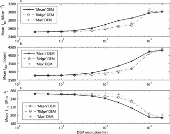
Fig. 6. Whole-glacier spatial mean values of (a) yearly total potential direct-beam solar radiation (I tot; MJ m −2), (b) yearly potential duration of direct-beam solar radiation (I dur; hours) and (c) mean intensity of potential direct-beam solar radiation (I int; W−2), for the three DEMs interpolation schemes. The tick marks denote the DEM resolutions used in this study. Note that given the range of DEM resolutions tested, the x-axis scale is logarithmic.
This pattern is repeated for the whole-glacier spatial mean of I dur (Fig. 6b, solid curve): a slow increase in the spatial mean at resolutions finer than ∼50 m, a more rapid increase as resolution coarsens to around 1000 m, then a slower increase up to the coarsest resolution, again approaching the planar value of 4541 hours. The impact is, however, even more marked; the increase from 2.5 to 200 m resolution is 583 hours, or 21% of the value from the 2.5 m DEM.
The greater proportional error in I dur compared with the error in I tot means that the whole-glacier spatial mean of intensity of potential direct-beam solar radiation (I int) is also affected by DEM resolution. However, for the spatial mean of I int (Fig. 6c, solid curve) the pattern effectively reverses: there is a slow decrease in the spatial mean I int as resolution coarsens to around 20 m, then a more rapid decrease to round 1000 m, before another slowing in the rate of decrease at the coarsest resolutions. The change from 2.5 to 200 m resolution is 21 W m−2, or 8% of the 2.5 m DEM value.
The changes in radiation receipt are considerable: the spatial mean value of I tot at 2.5 m resolution is 79% of the theoretical maximum received by a planar surface; at 50 m resolution, the value has increased by 90.2 MJ m −2, or 4%, to 82% of the value for a planar surface; at 200 m resolution, the calculated value has increased by 274.2 MJ m−2 (11%), to 88% of the maximum. Given the area of the glacier, the change from 2.5 to 200 m resolution is equivalent to melting an extra 3.93 × 10⁶ m3 of water, given the latent heat of fusion of ice. Assuming a 90 day melt season, this is the equivalent of ∼8 mm w.e. d−1, approximately half the longterm glacier-wide summer mass balance (Kohler and others, unpublished data). This is a maximum value; the impact on the overall energy balance will be less, as direct-beam solar radiation is not the only source of energy.
For the rotated DEMs, although the calculated values of I tot and I dur vary with the different DEM aspects, the changes for each aspect due to DEM resolution were almost identical to the changes in the ‘true’ aspect DEM. Between 2.5 and 200 m, the whole-glacier spatial mean of I tot increased by 11%, 9% and 9% of the value for the 2.5 m DEMs, and the whole-glacier spatial mean of I dur increased by 25%, 26% and 23% of the value for the 2.5 m DEMs for the east-, south-and west-facing aspect runs respectively.
Explanation of the impacts of DEM resolution on solar radiation receipts
The possible controls on I which will be affected by DEM resolution are the value of cos Θ (the local zenith angle of the solar beam) because of the possible impact of resolution on calculated local slope and aspect, and the influence of shading by the surrounding topography. Table 1 shows (1) the whole-glacier spatial means of derived topographic characteristics for the ‘mean’ DEM at the various DEM resolutions, (2) the spatial mean slope, (3) the spatial mean aspect (calculated from the aspect of each DEM cell using standard circular statistics), (4) the spatial mean local zenith angle (calculated from Equation (3), summed over the glacier surface and over the course of a year), (5) the spatial mean sky-view factor (calculated from Equation (4)) and (6) the spatial mean elevation. The spatial means of slope, aspect and local zenith angle show very small changes with DEM resolution, and no clear resolution dependency. However, the sky-view factor does show a clear increase as DEM resolution coarsens. This is not to say that calculated slope and aspect (and therefore local zenith angles) do not vary over the glacier at different DEM resolutions, but rather that the variations which do occur are masked when the spatial mean for the whole glacier is calculated, as some areas will have steeper slopes (e.g. near the edge of the glacier where there is an abrupt change in slope), and other areas may have shallower slopes (e.g. in central parts of the glacier where topography is already relatively smooth) at coarser resolutions.
Table 1. Derived topographic parameters for the ‘mean DEM’ at different spatial resolutions
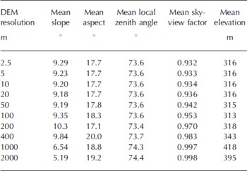
Altering the DEM cell centres also has no significant impact on these values; even at the finest resolution of 2.5 m, almost every DEM cell contains at least one lidar point. As resolution coarsens, the number of lidar points within each cell increases markedly. The altered cell centre means the slope and aspect in that cell are different from those calculated in the nearest equivalent cell for different cell centres, but these differences cancel out when the whole-glacier spatial means are calculated.
Slope, aspect and zenith-angle variations seem therefore to be responsible for the increased small-scale (<10 m) variability of I tot (Fig. 4) at fine DEM resolutions. They have much less effect on the small-scale variability on I dur, as shown by the lower ‘roughness’ of the plots at fine DEM scales in Figure 5. The very high latitude of the glacier also means that the sun will come from all compass directions during the ∼4 months of 24 hour daylight, as argued by Reference Arnold, Rees, Hodson and KohlerArnold and others (2006b). Thus, local ‘highs’ in I tot due to slope and aspect are cancelled out by ‘local’ lows with different slope/aspect combinations.
There is a limited effect of DEM resolution on the spatial mean values of slope, aspect and zenith angle. This and the marked relationship between the spatial mean of the sky-view factor and DEM resolution suggest that it is effectively the height of the ‘viewshed’ (i.e. the points which form the horizon from any given cell at any given angle) and therefore (in terms of the direct solar radiation) the degree of shading of the glacier surface that is responsible for the ‘offset’ between the values of I tot and I dur at the different DEM resolutions seen in Figures 4 and 5. The trends in the spatial means (Fig. 6) will also affect the ‘offset’. This is also supported by the experiments with the rotated DEMs. Although these show different total values due to aspect, the impact of resolution is almost identical to the ‘true’ aspect runs.
The prime cause of the radiation variations is the calculated I dur. Underestimation of shading at coarser resolutions leads to an increase in I tot, but a decrease in I int, because the excess radiation is at lower solar angles.
On rough ground, the assumption that the height of a gridcell is best represented as the mean of all the point measurements within that gridcell will effectively smooth the topography. Point measurements below or above the mean value will have their impact on the cell height reduced by the averaging. This problem will be most marked in areas of variable topography; troughs or peaks within the data will tend to be removed. This process will become more and more effective as the cell size increases. It is likely, then, that the reason for the overestimation of I dur over the glacier (and hence I tot) is the underestimation of the height of the ‘viewshed’ from any given location on the glacier surface. This would normally be the peaks and ridges which surround the glacier, and which cast shadows onto it, but it could also be lower but nearer topographic features which obscure the horizon from particular locations. This is also the explanation for the increase in the spatial mean elevation of the glacier surface. At the coarsest resolutions, the elevation of cells which represent the glacier (as opposed to the surrounding topography) will effectively include some measurements from the (generally higher) surrounding topography.
This spatial averaging also explains the tendency for the discrepancy between the various DEM resolutions to be more marked near the margins of the glacier, as these areas are most affected by shading by the surrounding high terrain. It also explains the smaller discrepancy for Transect A; this is low on the glacier, across the area where the glacier snout ‘protrudes’ onto the coastal plain, and hence is less affected by shading caused by the surrounding topography.
Impact of DEM resolution on total energy balance
The glacier-wide spatial means of the calculated total energy balance for the periods 25 April–12 September 2001–03 (m w.e. of melt, averaged over the three model runs) and the four energy-balance components (net solar and longwave radiative fluxes, and sensible and latent turbulent fluxes (W m−2) calculated by taking the glacier-wide spatial means of the total fluxes over the model runs for the three years, dividing by the run length, then averaging over the three model runs) at different DEM resolutions are shown in Figure 7. Although the magnitude of the spatial mean of total energy balance varies from year to year, the increase in total energy balance in all three years is very similar, at approximately 3% for a change in DEM resolution of 2.5–200 m. The calculated net solar radiative flux increases by approximately 5% in all three years as resolution coarsens from 2.5 to 200 m. At resolutions coarser than 100–200 m, however, the pattern changes: the spatial means of total energy balance and net solar radiative flux both begin to decrease. The other energy-balance components behave in a more monotonic way: the spatial mean of net longwave radiation becomes increasingly negative at coarser resolutions; the spatial mean of turbulent sensible heat flux becomes less positive at coarser resolutions; and the spatial mean of turbulent latent heat flux becomes increasingly negative at coarser resolutions.
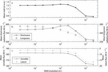
Fig. 7. Glacier-wide spatial mean values of (a) the total energy balance (m w.e. of melt), (b) net solar and longwave radiative fluxes (W m−2) and (c) sensible and latent heat fluxes (W m−2) at different DEM resolutions for the periods 25 April–15 September 2001–03. Data are the averages for the three model runs. The tick marks denote the DEM resolutions used in this study; as in Figure 6, the x-axis scale is logarithmic.
Explanation of the impact of DEM resolution on total energy balance
This difference in behaviours between the calculated net solar radiative flux and the total energy balance at different DEM resolutions, and the other energy-balance components, is explained by the increase in the spatial mean of the elevation of the glaciated cells (Table 1) at the coarsest resolutions.
Elevation affects the turbulent energy-balance components due to the impact of atmospheric lapse rates on air temperature. It also affects the net longwave flux through changes in surface temperature (which generally decreases with altitude) affecting the outgoing longwave flux, and through lower air temperature at high elevation reducing the downward flux. Elevation also affects net solar radiation receipts as it controls the modelled start-of-season snow depths. The mean surface albedo is therefore higher at coarser DEM resolutions (Equation (5)), which reduces the net solar radiative flux in spite of the increase in potential radiation at coarser resolutions. In order to try to isolate the impact of topographic resolution and potential solar radiation availability on the overall energy balance, we concentrate the discussion here on the changes at resolutions finer than 200 m. These seem to be affected mainly by the direct impact of DEM resolution on solar radiation receipt, since the spatial mean of surface elevation is similar at DEM resolutions finer than 200 m. We also break the discussion down and examine the impact of resolution on net solar radiation receipt, before considering the interactions between the various energy-balance components.
The reduction in sensitivity to resolution of the net solar radiative flux compared with I tot has two main causes. First, the modelled I tot is a maximum value. Absorption by clouds, in particular, is not accounted for in the potential radiation calculations. Such absorption will reduce the direct-beam component of solar radiation received by the surface, and therefore the total radiation receipts over a given time period. Diffuse radiation will form the bulk of the solar radiation receipt during cloudy weather. This is unaffected by shading by the surrounding topography, although it is affected by the sky view. Midre Lovénbreen experiences a relatively cloudy climate (hence the relatively small number of clear-sky observations discussed in the validation section above). Thus net solar radiation is less sensitive to DEM resolution than potential direct-beam solar radiation.
Second, however, and acting against this, is the well-documented reduction in surface albedo as snow melts, calculated in the model with Equation (5). This means that all other factors being equal, a snow surface receiving more solar radiation will melt faster, and hence show a more rapid albedo decrease than one receiving less radiation. It will thus exhibit a lower mean albedo over a given time period. This serves to increase the impact of DEM resolution on net solar radiation receipts. The first effect seems to dominate in our study, and the overall sensitivity of net solar radiation (and total energy balance) to DEM resolution is lower than for the potential direct-beam solar radiation.
In terms of the total energy balance, the impact of DEM resolution is complicated by the interplay between the various sources and sinks of energy that have been observed over glaciated surfaces (e.g. Reference Bintanja, Jonsson and KnapBintanja and others, 1997; Reference Arnold, Rees, Hodson and KohlerArnold and others, 2006b), and which affect the rates of snowmelt and the overall energy balance. Reference Arnold, Rees, Hodson and KohlerArnold and others (2006b) argue that an increase in any given component can lead to a reduction in one of the other components of the surface energy balance through changes in the glacier surface temperature (e.g. an increase in the surface temperature (due, for example, to greater solar radiation receipts) leads to an increase in the outgoing flux of longwave radiation). Such negative feedback effects seem to be responsible for the reduction in sensitivity of the total energy balance to DEM resolution in our results (e.g. overall mean longwave radiation receipts become more negative at coarser resolutions (due to higher surface temperatures), to some extent offsetting (in terms of the total energy balance) the increase in solar radiation receipts at these resolutions.
Mitigation of resolution effects
Given the impact of errors in shading calculations at different DEM resolutions, we performed two more sets of calculations using the ‘ridge’ and ‘maximum’ DEMs described above. Figure 8 shows I tot for the four transects for the ‘ridge’ DEM (the values for the ‘maximum’ DEM are very similar, and are not shown). Except at the coarsest resolution shown (200 m), these generally show a much closer agreement between the fine- and coarse-resolution DEMs. Detail is lost at coarser resolutions, but the overall fit is much improved.
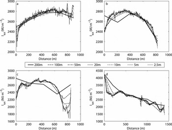
Fig. 8. Yearly total potential direct-beam solar radiation (I tot; MJ m−2) for the four transect locations shown in Figure 1 at different DEM resolutions, based on the ridge DEMs.
This improvement is borne out in Figure 6 (dashed and dotted curves), which shows the whole-glacier spatial mean values of I tot, the spatial mean of I dur and the spatial mean of I int for the ‘ridge’ and ‘maximum’ DEMs. These show a change in the scale dependency compared with the ‘mean’ DEMs. The curves are still broadly sigmoid in shape, but the ‘flatter’ section of the curves extends to coarser resolutions before the rapid change in the calculated values sets in at resolutions coarser than around 50–100 m. At the very coarsest resolutions, the DEM generation algorithm has little impact, however. Indeed, the ‘maximum’ DEM seems to produce a large overestimate in I tot at 2000 m resolution.
Conclusions
We have presented the results of a set of distributed calculations of year-long solar radiation totals over a small valley glacier in the High Arctic, midre Lovénbreen. These calculations have clearly shown that as well as the intuitive reduction in the spatial resolution of distributed energy-balance calculations, too coarse a DEM resolution can lead to:
a profound overestimation of the calculated total amount of potential direct-beam solar radiation (by 20% between the finest (2.5 m) and coarsest (2000 m) resolutions);
a profound overestimation of the calculated total potential duration of direct-beam solar radiation (by 56%);
an underestimation of the calculated mean intensity of potential direct-beam solar radiation (by 23%) over a glaciated surface in mountainous terrain.
Experiments with rotated DEMs have shown that these effects are largely independent of the overall aspect of the glacier.
DEM resolution similarly affects the net solar radiative flux, and thus the season-long total modelled energy balance and, hence, modelled melt. The impact of DEM resolution on the overall season-long total energy balance can be as high as 30% at very coarse resolutions (2000 m) compared with the finest resolutions (2.5 m). At a 3–5% difference between the 2.5 and 200 m resolutions, however, the impact of DEM resolution is broadly comparable with the tests in other studies that have examined the impact of slope, aspect and shading on energy-balance calculations (e.g. Reference Arnold, Willis, Sharp, Richards and LawsonArnold and others, 1996; Reference Klok and OerlemansKlok and Oerlemans, 2002; Reference Arnold, Rees, Hodson and KohlerArnold and others, 2006b). Thus, the DEM resolution adopted in energy-balance models can in itself lead to errors comparable with those associated with omitting topographic effects entirely.
The principal cause of these errors is changes in the calculated patterns of shading at coarser DEM resolutions. The glacier surface in the coarse-resolution DEMs spends too long ‘in sun’, typically at lower solar elevations, which increases the total potential direct-beam solar radiation receipt (through the increased potential duration of direct-beam solar radiation. However, this reduces the mean potential direct-beam solar radiation intensity. Thus, at coarser resolutions, modelled direct-beam solar radiation receipts will begin (or increase) earlier in the summer and earlier in each day. Modelled receipt of direct solar radiation will decrease (or cease) later in the melt season and later each day.
Calculations of diffuse solar radiation receipts and incoming longwave radiation receipts are similarly affected because the calculations of the sky-view factor are also strongly controlled by DEM resolution, changing by 7% of the 2.5 m value between the finest (2.5 m) and coarsest (2000 m) resolutions. Diffuse solar radiation is generally a very minor component of the energy balance of a glaciated surface (although Reference Klok and OerlemansKlok and Oerlemans (2002) show that obstruction of the sky by the surrounding terrain reduces calculated solar radiation by 6.7% for Morteratschgletscher, Switzerland). However, incoming longwave radiation can be a major contributor of energy, making potential errors more serious.
On the other hand, we have shown that it is possible to mitigate these impacts quite easily at DEM resolutions finer than ∼50 m by the simple expedient of ensuring that the ‘viewshed’ surrounding the glacier is as accurately represented as possible. The impact of resolution can be reduced by simply ensuring that the height of ridges and peaks surrounding the catchment is accurately represented in the DEM. Even in areas without comprehensive high-resolution topographic data, the simple expedient of taking ridge and peak heights from large-scale topographic maps will improve estimates of solar radiation loading. Where intensively sampled topographic data are available, using the maximum value rather than the mean value in all DEM cells gives a further subtle improvement, though only at finer resolutions.
Our results suggest that for valley glaciers of similar size to midre Lovénbreen, and in similarly mountainous terrain, ∼50 m spatial resolution is the coarsest DEM resolution which should ideally be used in spatially distributed surface energy-balance calculations. A 20 or 30 m spatial resolution would be better if good maps, surveys or other topographic data are available for the area. Where possible, such DEMs should give the maximum height for the topographic high points surrounding the glacier, rather than a mean or interpolated height for each DEM cell. Accurate representation of these heights becomes more important as resolution coarsens.
This resolution limit needs to be finer for areas with a higher overall relief, as shading will be more dominant. It could be relaxed for larger glaciers, or those in areas of smaller overall relief, as patterns of shading will affect a smaller proportion of the glacier in these circumstances. We see no reason to assume that these findings will not apply in other catchments in areas of high relief, whether glaciated or not, as the effect we have demonstrated is a product of the interaction between solar and catchment geometries and DEM resolution.
Acknowledgements
N.S.A. and W.G.R. were funded by the Scott Polar Research Institute, the University of Cambridge and St John’s and Christ’s College, the University of Cambridge. J. Kohler of the Norsk Polarinstitutt kindly provided unpublished mass-balance data for midre Lovénbreen. The UK Natural Environment Research Council (NERC) Airborne Remote Sensing Facility and the University of Cambridge Unit for Landscape Modelling provided the lidar data. N.S.A. and W.G.R. stayed at the NERC Arctic Research Station, and we thank the base manager N. Cox and his deputies for their logistic support. We also thank the various reviewers and the Scientific Editor, R. Hock, for comments. Figure 1 is based on digital spatial data licensed from the Natural Environment Research Council ©NERC 2005.


