


1. Introduction
If we shake a bottle of water violently, the entrapped air forms bubbles of different sizes, which rise vertically due to buoyancy and burst when they reach the upper water–air interface. The in-depth understanding of bubble dynamics, not only in Newtonian (Tsamopoulos et al. Reference Tsamopoulos, Dimakopoulos, Chatzidai, Karapetsas and Pavlidis2008) but also in complex fluids (Dimakopoulos, Pavlidis & Tsamopoulos Reference Dimakopoulos, Pavlidis and Tsamopoulos2013; Fraggedakis et al. Reference Fraggedakis, Pavlidis, Dimakopoulos and Tsamopoulos2016; Moschopoulos et al. Reference Moschopoulos, Spyridakis, Varchanis, Dimakopoulos and Tsamopoulos2021), is required by their presence in numerous industrial processes and daily applications. For example, the effective control of bubbles in foods improves their texture (Campbell Reference Campbell1999). How bubbles grow, deform and form fibrils constitutes an important feature of the debonding process of self-adhesives or pressure-sensitive adhesives (PSAs) (Varchanis et al. Reference Varchanis, Kordalis, Dimakopoulos and Tsamopoulos2021a) and controls their tackiness. Bubbles are desirable in some applications, like chemical or biochemical reactors, because they facilitate mass transfer. Furthermore, the mechanical properties of construction concrete may degrade significantly by their presence, necessitating their almost complete removal. These cases demonstrate the importance of accurately understanding bubble dynamics, especially in complex materials.
The motion of bubbles in viscoelastic materials has been a subject of intense research for over six decades. The coupled effects of elasticity and deformation of the bubble interface generate an abundance of astonishing phenomena. Throughout the years, three intriguing observations emerge that do not have any correspondence in the translation of bubbles in Newtonian fluids: (a) the velocity jump discontinuity; (b) the negative wake behind the bubble and (c) the knife-edge shape of a bubble.
In their pioneering work, Astarita & Apuzzo (Reference Astarita and Apuzzo1965) were the first to report an abrupt, almost ten-fold increase in the speed of a bubble once its volume surpassed a critical value. This increase was so intense that the term ‘jump’ was used to characterize it because two separate and distinct curves of stationary solutions were obtained. Subsequent experiments verified these observations and established that the velocity jump was approximately 6–10 times for shear-thinning viscoelastic solutions. Still, it was much less in Boger fluids, namely constant viscosity viscoelastic solutions. Leal, Skoog & Acrivos (Reference Leal, Skoog and Acrivos1971) conducted an early numerical work and they solved the creeping flow of an inelastic, shear-thinning material around a spherical bubble. They concluded that the shear thinning viscosity contributed to the increase of the rising velocity but was not the key factor that could lead to the velocity jump. A coherent physical mechanism for the velocity jump discontinuity was proposed by Fraggedakis et al. (Reference Fraggedakis, Pavlidis, Dimakopoulos and Tsamopoulos2016). They performed steady-state simulations with arclength continuation techniques, and captured the two distinct solution branches and a hysteresis loop connecting them. Their numerical results showed that when the critical bubble volume was surpassed, significant hoop stresses intensified the developed shear layer at the trailing pole of the bubble, which thrusted it vertically. Also, the shear-thinning nature of the material decreased the flow resistance in the front of the bubble, which allowed it to rise faster. These findings were confirmed by Niethammer et al. (Reference Niethammer, Brenn, Marschall and Bothe2019).
In his study, Hassager (Reference Hassager1979) revealed an uncommon flow structure behind the rising bubble: only a small portion of the fluid just behind the trailing pole of the bubble followed it, a stagnation point appeared further down, and most of the fluid below the stagnation point and around the axis of symmetry moved downwards. So, most of the material under the bubble flowed in the opposite direction of the motion of the bubble, a phenomenon that was contrary to what was observed for objects translating in Newtonian fluids. He termed it ‘negative’ wake. Ensuing works demonstrated the universality of the negative wake structure (Bisgaard & Hassager Reference Bisgaard and Hassager1982), which was observed in flows of bubbles and around spheres or cylinders. The flow around a sphere or a cylinder was much easier to study, both experimentally and numerically. Hence, the negative wake was investigated intensively in these flows. However, the ensuing studies were contradictory because the negative wake occurred in some polymeric fluids, whereas it was absent from others. The negative wake appeared only in flows of shear-thinning, viscoelastic materials (Maalouf & Sigli Reference Maalouf and Sigli1984; Arigo et al. Reference Arigo and Mckinley1998) but not in Boger fluids (Arigo et al. Reference Arigo, Rajagopalan, Shapley and Mckinley1995). Contradictory conclusions were also drawn from simulations regarding the nature of the negative wake (Chilcott & Rallison Reference Chilcott and Rallison1988; Satrape & Crochet Reference Satrape and Crochet1994). Finally, Harlen (Reference Harlen2002) concluded that the negative wake was governed by a delicate balance of two competing viscoelastic forces: the extensional forces in the birefringent strand downstream lengthened the decay of the fluid velocity and an extended wake arose. Simultaneously, shear forces in a region surrounding the strand induced an elastic recoil, pulled the material away from the sphere and produced a negative wake.
Inevitably, the surface of bubbles deformed when they translated through a fluid, either Newtonian or non-Newtonian. Since the work of Astarita & Apuzzo (Reference Astarita and Apuzzo1965), it was established that the shape of the bubbles transitioned from a convex to an inverted tear drop shape when their volume increased. This transition occurred approximately at the critical volume for the onset of the velocity jump discontinuity. Chilcott & Rallison (Reference Chilcott and Rallison1988) simulated a ‘cylindrical’ bubble using the FENE-CR model and suggested that the strong viscoelastic, normal stresses developed in the trailing pole were responsible for the teardrop bubble observed in experiments. However, they did not allow for any surface deformation and they did not capture numerically the experimentally observed shape. Later, Noh, Kang & Leal (Reference Noh, Kang and Leal1993) performed detailed simulations accounting for the deformation of the bubble surface using a boundary-fitted coordinate system. They captured the inverted teardrop shape and deduced that the strong uniaxial elongational flow behind the bubble created it. Eventually, many numerical works that dealt with the bubble rise in a viscoelastic solution presented the inverted teardrop shape, either employing the finite-elements method (Fraggedakis et al. Reference Fraggedakis, Pavlidis, Dimakopoulos and Tsamopoulos2016; Varchanis & Tsamopoulos Reference Varchanis and Tsamopoulos2022) or the finite-volume method (Niethammer et al. Reference Niethammer, Brenn, Marschall and Bothe2019; Yuan et al. Reference Yuan, Zhang, Khoo and Phan-Thien2020, Reference Yuan, Zhang, Khoo and Phan-Thien2021).
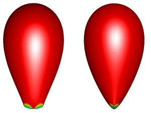
The last chapter of unravelling the bubble rise problem concerns the astonishing knife-edge bubble shape, as shown in figure 1, and was reported initially by Hassager (Reference Hassager1979). This unique asymmetric shape emerges in situations that one would normally expect an axisymmetric one. Instead, a sharp, two-dimensional, cusp-like tail forms in one view (figure 1a), but it turns into a broad knife or a spade in the orthogonal view (figure 1b). From this point forward, we shall refer to it with the term ‘two-dimensional cusp’ as an effective cusp that has a very small, but finite size and rounded tip. Liu, Liao & Joseph (Reference Liu, Liao and Joseph1995) (referred to hereafter as LLJ) investigated thoroughly the emergence of the knife edge for different viscoelastic materials. They reported that all bubbles attain the knife-edge shape irrespective of the material or the experimental set-up. The type of cross-section of the column, either square or cylindrical, affects the orientation of the cusp edge. They identified a preference of the direction of the cusp edge in rectangular containers depending on whether the bubble volume is below or above a specific threshold. Sometimes, the shape of the knife edge alters from a spade to an axe depending on the bubble volume, the material and the size of the container. Even arrow or guillotine shapes were reported by LLJ (see their figure 1). Also, these configurations are observed to be steady. The interface did not oscillate and the bubble translated with a constant speed. To the authors’ knowledge, this unusual shape has not been reported in any subsequent experimental work, owing probably to the very specific range of parameters that enables its appearance. Even though some numerical studies (Yuan et al. Reference Yuan, Zhang, Khoo and Phan-Thien2020, Reference Yuan, Zhang, Khoo and Phan-Thien2021) tackled the problem of a rising bubble in a three-dimensional setting, they did not report any asymmetric shapes. In this brief review of the relevant literature, we do not include studies of bubbles rising in surfactant or associative polymer solutions, or studies in which the density and viscosity ratios between the liquid and its inclusion excluded the presence of a gas in it. The work of Fraggedakis et al. (Reference Fraggedakis, Pavlidis, Dimakopoulos and Tsamopoulos2016) assumed axial symmetry; so, it excluded any azimuthal variations. Following a different approach, You, Borhan & Haj-Hariri (Reference You, Borhan and Haj-Hariri2009) simulated the axisymmetric case using the FENE-CR model and then performed a linear stability analysis on the base state they obtained. They concluded that the only unstable eigenmode has a zero imaginary part and an azimuthal wavenumber equal to 2, which could lead to the formation of the steady knife edge, when nonlinearities prevail. However, a three-dimensional simulation that captures the knife edge is missing from the literature.

Figure 1. Schematic of the lower part of the knife-edge shape. Two mutual orthogonal views are shown: (a) the cusp-like tip and (b) the knife edge.
In this work, we revisit the dynamics of a bubble rising though a viscoelastic material. The novel aspect of this study is that we do not assume axial symmetry but solve numerically the complete, three-dimensional form of the governing equations. We use the recently developed finite-element framework for free surface flows of non-Newtonian fluids by Varchanis et al. (Reference Varchanis, Syrakos, Dimakopoulos and Tsamopoulos2019, Reference Varchanis, Syrakos, Dimakopoulos and Tsamopoulos2020c). We compare the computed bubble shape with the experimental ones from the work of Liu et al. (Reference Liu, Liao and Joseph1995). In most cases, we achieve quantitative agreement with the experiments and predict the experimentally observed knife-edge shape. Furthermore, we address some important questions regarding the knife-edge shape. How are the kinematics of the flow altered to enable such an asymmetric shape? Does the bubble deformability facilitate the creation of the knife edge? What is the extensional character of the fluid that allows the emergence of this shape? Even more generally, which rheological properties, shear or extensional, steady or transient, lead to the knife-edge shape? Does the appearance of this shape lead to a change in the speed of the bubble or even a velocity jump? Finally, is the knife-edge shape a purely elastic instability and how is it affected by the blockage ratio, defined as the bubble to cylinder radius ratio? Along with the answers to the posed questions, we offer insights into the mechanism that governs the transition from an axisymmetric solution to an asymmetric one.
Our study is divided as follows. In § 2, we formulate the physical problem and introduce the governing equations, followed by their corresponding boundary conditions. In § 3, we outline briefly the employed numerical method. In § 4, we determine the rheological properties of the materials used in the experiments of LLJ. In § 5, we report the comparison of our novel numerical results with the experimental ones. Furthermore, we conduct a parametric study and present our proposed mechanism that leads to the knife-edge shape. Finally, we draw conclusions in § 6.
2. Problem formulation
We investigate the buoyancy-driven rise of a bubble of volume  ${\tilde{V}_b}$ that translates steadily upwards with speed ${\tilde{U}_b}$ along the axis of a cylindrical container with a radius ${\tilde{R}_C}$, filled initially with a viscoelastic material (shown schematically in figure 2). The viscoelastic material is incompressible with constant density $\tilde{\rho }$, zero-shear rate viscosity, ${\tilde{\eta }_0}$, and relaxation time, $\tilde{\lambda }$. A tilde $(\ \widetilde {}\ )$ denotes a dimensional variable or parameter, whereas the absence of one denotes its dimensionless counterpart. We assume that the density and the viscosity of the bubble are negligible compared with the respective ones of the surrounding material. The surface tension, $\tilde{\sigma }$, of the liquid–gas interface is spatially uniform and constant. We adopt a cartesian coordinate system, $\{ \tilde{x},\tilde{y},\tilde{z}\} $, where the $\tilde{z}$ direction is aligned along the gravity vector, $\tilde{\boldsymbol{g}}$, which points to the negative direction, namely $\tilde{\boldsymbol{g}} ={-} \tilde{g}{\boldsymbol{e}_z}$. Instead of using the above-described inertial frame, we simulate the flow in a reference frame moving with the bubble. Hence, we position the centre of the coordinate system at the centre of volume of the bubble, so it moves upwards with the bubble in the inertial frame. This selection renders the bubble stationary, and the surrounding fluid and container translate downwards with speed (i.e. velocity magnitude), ${\tilde{U}_f}$, which is equal to the actual bubble speed, ${\tilde{U}_b}$.

Figure 2. Schematic of the rising bubble though a viscoelastic material under gravity. Here,  ${S_X}$ and ${S_Y}$ denote the symmetry plane at $\tilde{x} = 0$ and $\tilde{y} = 0$, respectively; ${S_f}$, ${S_T}$, ${S_o}$ and ${S_C}$ denote the fluid/gas interface, the top boundary, the bottom boundary and the cylindrical wall boundary, respectively. The origin of the coordinate system is in the centre-of-volume of the bubble and translates with it.
Note that we do not assume axial symmetry and we solve the full, three-dimensional problem. To reduce the high computational cost to solve this problem, we assume two planes of symmetry, one at  $\tilde{x} = 0({S_X})$ and a second one at $\tilde{y} = 0({S_Y})$, and compute the flow in one-fourth of the domain. Our choice not only reduces the computational cost but is also based on the experimental observations of LLJ, where similar planar symmetry arises. Another desired outcome of having two symmetry planes is that we restrain the bubble from shifting in the $\tilde{x}$ and $\tilde{y}$ directions, focusing on its vertical motion only. There is no experimental indication that the appearance of the knife-edge shape is a result of such motion.
We adopt the non-dimensionalization proposed in the works of Fraggedakis et al. (Reference Fraggedakis, Pavlidis, Dimakopoulos and Tsamopoulos2016) and Tsamopoulos et al. (Reference Tsamopoulos, Dimakopoulos, Chatzidai, Karapetsas and Pavlidis2008). We scale lengths with the equivalent bubble radius,  ${\tilde{R}_b} = {(3{\tilde{V}_b}/4{\rm \pi})^{1/3}}$, and velocities by balancing viscous forces to buoyancy, i.e. ${\tilde{U}_{vg}} = \tilde{\rho }\tilde{g}\tilde{R}_b^2/{\tilde{\eta }_0}$. We choose this velocity scaling for two reasons, as explained previously (Tsamopoulos et al. Reference Tsamopoulos, Dimakopoulos, Chatzidai, Karapetsas and Pavlidis2008; Fraggedakis et al. Reference Fraggedakis, Pavlidis, Dimakopoulos and Tsamopoulos2016). First, it allows following closely the experimental protocols, where the bubble volume is varied, and the terminal velocity is measured subsequently. Second, it permits determining the velocity of the bubble as part of the solution for a set of material properties and bubble volume, and not imposing it beforehand. It follows naturally that pressure and stresses are scaled with $\tilde{\rho }\tilde{g}{\tilde{R}_b}$. Based on the above considerations, three dimensionless numbers and a geometric ratio arise: $Ar,Bo,Eg,{B_R}$, given by
 \begin{equation}Ar = \frac{{{{\tilde{\rho }}^2}\tilde{g}\tilde{R}_b^3}}{{{{\tilde{\eta }}_0}}},\quad Bo = \frac{{\tilde{\rho }\tilde{g}\tilde{R}_b^2}}{{\tilde{\sigma }}},\quad Eg = \frac{{\tilde{\lambda }\tilde{\rho }\tilde{g}{{\tilde{R}}_b}}}{{{{\tilde{\eta }}_0}}}\left( { \equiv \frac{{\tilde{\lambda }}}{{{{\tilde{t}}_{vg}}}} = \frac{{\tilde{\lambda }{{\tilde{U}}_{vg}}}}{{{{\tilde{R}}_b}}}} \right),\quad {B_R} = \frac{{{{\tilde{R}}_b}}}{{{{\tilde{R}}_c}}}\textrm{.}\end{equation}
The first one is the Archimedes number, which is the ratio of inertial forces to gravity. It can be interpreted as a modified Reynolds number where the velocity scale is given by  ${\tilde{U}_{vg}}$. The second is the Bond number, which measures the importance of gravity to capillarity. The third one is the elastogravity number, which appears due to the elastic properties of the material. It is the ratio of the relaxation time of the fluid to the characteristic residence time in the flow, ${\tilde{t}_{vg}} = {\tilde{R}_b}/{\tilde{U}_{vg}}$ (the viscous-gravity time scale) and quantifies the importance of elastic effects. The last one is the ratio of the bubble radius to the cylinder radius, the so-called blockage ratio.
Using the previous arguments, the dimensionless governing equations for the momentum and mass conservation take the following form:
 \begin{gather}Ar\boldsymbol{u}\boldsymbol{\cdot }\boldsymbol{\nabla }\boldsymbol{u} - \boldsymbol{\nabla }\boldsymbol{\cdot }\boldsymbol{T} + {\boldsymbol{e}_Z} = 0,\end{gather}
 \begin{gather}\boldsymbol{\nabla }\boldsymbol{\cdot }\boldsymbol{u} = 0,\end{gather}
where  $\boldsymbol{\nabla }$ denotes the usual gradient operator, $\boldsymbol{u}$ is the velocity vector, and $\boldsymbol{T}$ is the Cauchy stress tensor, which is split into the pressure and the extra stress tensor as $\boldsymbol{T} ={-} P\boldsymbol{I} + \boldsymbol{\tau }$. The last term on the left-hand side of (2.2) represents the dimensionless gravity force. The extra stress tensor follows the exponential Phan-Thien–Tanner (e-PTT) model (Phan-Thien & Tanner Reference Phan-Thien and Tanner1977; Phan-Thien Reference Phan-Thien1978), which can be expressed in dimensionless form as
 \begin{equation}Eg
\mathop{\boldsymbol{\tau}}\limits^\nabla +\, Y(tr(\boldsymbol{\tau
}))\boldsymbol{\tau } = \dot{\boldsymbol{\gamma
}},\end{equation}
\begin{equation}Eg
\mathop{\boldsymbol{\tau}}\limits^\nabla +\, Y(tr(\boldsymbol{\tau
}))\boldsymbol{\tau } = \dot{\boldsymbol{\gamma
}},\end{equation}
where ‘ $tr(\boldsymbol{\tau })$’ denotes the trace of the tensor $\boldsymbol{\tau }$, and the rate-of-strain tensor $\dot{\boldsymbol{\gamma }}$ is defined as $\dot{\boldsymbol{\gamma }} = \boldsymbol{\nabla }\boldsymbol{u} + {(\boldsymbol{\nabla }\boldsymbol{u})^T}$. The function $Y(tr(\boldsymbol{\tau }))$ of the e-PTT model reads as
 \begin{equation}Y(tr(\boldsymbol{\tau })) = \exp ({\varepsilon _{PTT}}Egtr(\boldsymbol{\tau })),\end{equation}
where  ${\varepsilon _{PTT}}$ controls the strain-rate thinning of the material. When ${\varepsilon _{PTT}} \to 0$, the model reduces to the Oldroyd-B model. We also study other rheological models and give their expressions in Appendix A. More information regarding the rheological characterization of the materials is given in the following section and in Appendix A. Also, we disregard the viscous effects of the solvent because they are negligible for the material investigated by LLJ.
The upper convected derivative is defined as
 \begin{equation}\mathop{\boldsymbol{\tau }}\limits^\nabla = \boldsymbol{u}\boldsymbol{\cdot }\boldsymbol{\nabla }\boldsymbol{\tau } - {(\boldsymbol{\nabla }\boldsymbol{u})^T}\boldsymbol{\cdot }\boldsymbol{\tau } - \boldsymbol{\tau }\boldsymbol{\cdot }\boldsymbol{\nabla }\boldsymbol{u}.\end{equation}
Note that in both (2.6) and (2.2), we exclude the time derivative of the stresses and velocities, respectively, because we directly simulate the steady state of the system of partial differential equations (PDEs).
The above system of equations can be solved when appropriate boundary conditions accompany it. Along the bubble surface,  ${S_f}$, the velocity field satisfies a local force balance between pressure, viscous and elastic stresses in the liquid, surface tension of the interface, and the pressure inside the bubble, which reads
 \begin{equation}\boldsymbol{n}\boldsymbol{\cdot }\boldsymbol{T} ={-} {P_b}\boldsymbol{n} + B{o^{ - 1}}(2H)\boldsymbol{n},\ \textrm{on}\ {S_f},\end{equation}
where  $\boldsymbol{n}$ denotes the outward (with respect to the liquid) unit vector normal to the free surface ${S_f}(t)$, $2H ={-} {\nabla _s}\boldsymbol{\cdot }\boldsymbol{n}$ is the mean curvature of the free surface, ${\nabla _s} = (\boldsymbol{I} - \boldsymbol{nn})\boldsymbol{\cdot }\boldsymbol{\nabla }$ denotes the surface gradient operator and ${P_b}$ is the pressure of the bubble. Also, along the same boundary, we impose the kinematic boundary condition:
 \begin{equation}\boldsymbol{n}\boldsymbol{\cdot }\boldsymbol{u} = 0,\ \textrm{on}\ {S_f},\end{equation}
which, at steady state, is nothing more than the no-penetration condition.
We solve for the one-fourth of the domain; thus, we impose the plane of symmetry conditions along  ${S_X}$ and ${S_Y}$:
 \begin{gather}{\boldsymbol{n}_s}\boldsymbol{\cdot }\boldsymbol{T}\boldsymbol{\cdot }{\boldsymbol{t}_s} = 0,\ \textrm{on}\ {S_X}\ \textrm{and}\ {S_Y},\end{gather}
 \begin{gather}{\boldsymbol{n}_s}\boldsymbol{\cdot }\boldsymbol{u} = 0,\ \textrm{on}\ {S_X}\ \textrm{and}\ {S_Y},\end{gather}
where  ${\boldsymbol{n}_s}$, ${\boldsymbol{t}_s}$ are the unit normal and tangent vectors, respectively, to the ${S_X}$ and ${S_Y}$ planes. The no slip and no penetration boundary conditions are applied along the container walls, ${S_C}$:
 \begin{equation}\boldsymbol{u} ={-} {U_f}{\boldsymbol{e}_z},\ \textrm{on}\ {S_C}.\end{equation}
Unperturbed material flows into the domain from the top boundary,  ${S_T}$,
 \begin{gather}\boldsymbol{u} ={-} {U_f}{\boldsymbol{e}_z},\ \textrm{on}\ {S_T},\end{gather}
 \begin{gather}\boldsymbol{\tau } = 0,\ \textrm{on}\ {S_T},\end{gather}
while it exits from the bottom boundary,  ${S_o}$, where we apply the open boundary condition (OBC) of Papanastasiou, Malamataris & Ellwood (Reference Papanastasiou, Malamataris and Ellwood1992). The total height of the container is selected to minimize the effects of the location of the top and bottom boundaries. Moreover, the OBC allows us to place the bottom boundary closer to the bubble without affecting the numerical approximation of the problem and reducing further the computational cost of the simulations.
In the present formulation, we do not solve for the flow inside the bubble. Thus, we calculate the pressure of the air inside the bubble, constraining its volume to be constant and equal to  $4{\rm \pi}/3$. In the experiments of LLJ, the bubble travels a small distance and the assumption that the bubble pressure remains constant is quite accurate. The bubble volume can be evaluated efficiently using the following expression:
 \begin{equation}V ={-} \frac{1}{3}\int {\boldsymbol{n}\boldsymbol{\cdot }{\boldsymbol{r}_f}\,\textrm{d}{S_f}} ,\end{equation}
where  ${r_f}$ is the position vector of the free surface.
Finally, we determine  ${U_f}$ from the requirement that the centre of the volume of the bubble, ${z_{cv}}$, remains at the origin of the cartesian coordinate system:
 \begin{equation}{z_{cv}} \equiv \frac{3}{4}\frac{{\int {z(\boldsymbol{n}\boldsymbol{\cdot }{\boldsymbol{r}_f})\,\textrm{d}{S_f}} }}{{\int {\boldsymbol{n}\boldsymbol{\cdot }{\boldsymbol{r}_f}\,\textrm{d}{S_f}} }} = 0.\end{equation}
Note that the divergence theorem has been used to transform the volume integrals in (2.14) and (2.15) into surface integrals that can be evaluated on  ${S_f}$.
3. Numerical implementation
3.1. Finite-element formulation
We adopt a new finite-element formulation to numerically solve the preceding system of equations. The method was developed by Varchanis et al. (Reference Varchanis, Syrakos, Dimakopoulos and Tsamopoulos2019, Reference Varchanis, Syrakos, Dimakopoulos and Tsamopoulos2020c) for confined and free surface flow problems. Its crucial advantage is that equal order interpolants are admissible for all variables by generalizing the PSPG formulation (Hughes, Franca & Balestra Reference Hughes, Franca and Balestra1986) to viscoelastic materials, leading to a considerable reduction of the numerical cost, enhanced numerical stability compared with the standard mixed finite-element formulation and simpler code development. Moreover, it uses the DEVSS numerical scheme (Guénette & Fortin Reference Guénette and Fortin1995) to preserve the elliptic nature of the momentum equation even in the absence of a Newtonian solvent. It incorporates also the SUPG formulation (Brooks & Hughes Reference Brooks and Hughes1982) to handle the hyperbolic character of the constitutive model equation. The weak form of the momentum and mass balance equations and the constitutive model along with the implementation of the free surface boundary conditions can be found in Varchanis et al. (Reference Varchanis, Syrakos, Dimakopoulos and Tsamopoulos2020c). The method has been already successfully implemented for the solution of several benchmark problems, and for other critical flows of viscoelastic (Varchanis et al. Reference Varchanis, Pettas, Dimakopoulos and Tsamopoulos2021b) and elastoviscoplastic materials (Varchanis et al. Reference Varchanis, Haward, Hopkins, Syrakos, Shen, Dimakopoulos and Tsamopoulos2020a; Kordalis et al. Reference Kordalis, Varchanis, Ioannou, Dimakopoulos and Tsamopoulos2021; Moschopoulos et al. Reference Moschopoulos, Spyridakis, Varchanis, Dimakopoulos and Tsamopoulos2021, Reference Moschopoulos, Kouni, Psaraki, Dimakopoulos and Tsamopoulos2023). Although the aforementioned problems deal with two-dimensional geometries, the generalization to three dimensions is straightforward.
We approximate all variables with linear, four-node Lagrangian basis functions. We use an interface tracking technique to resolve the dynamics of the free surface. Thus, our implementation falls under the category of the arbitrary Lagrangian–Eulerian (ALE) methods and we choose the elliptic grid generation scheme proposed by Dimakopoulos & Tsamopoulos (Reference Dimakopoulos and Tsamopoulos2003) to control the motion of the internal nodes. As computational domain, we choose the volume that the liquid would occupy if the bubble remained spherical. Hence, the physical and computational mesh nodes have identical coordinates in the first step of the continuation procedure. A system of quasi-elliptic, nonlinear equations maps the deformed physical domain  $(x,y,z)$ to the simpler, undeformed and time-independent computational $(\xi ,\eta ,\zeta )$ one. For more details regarding the implementation of the grid generation scheme, the interested reader may refer to the works of Chatzidai et al. (Reference Chatzidai, Giannousakis, Dimakopoulos and Tsamopoulos2009) and Dimakopoulos & Tsamopoulos (Reference Dimakopoulos and Tsamopoulos2003).
3.2. Solution procedure
We discretize the domain using tetrahedral elements. Initially, we create a structured mesh of hexahedral elements that are subsequently split into five tetrahedrons each. We prefer tetrahedral elements over hexahedral ones because they conform better to severe deformations. After the creation of the mesh, we perform a systematic mesh convergence study to determine the optimal mesh discretization. To do so, we perform the same simulation with three different meshes, where we develop the two finer meshes by sequentially increasing the elements of the previous mesh in all directions by a factor of 1.5. In two-dimensional simulations, the computational burden permits us to double the mesh in both directions sequentially, but this increase would cause the computational cost to soar in three-dimensional simulations.
The largest discretization that we can use is of the order of 280 K nodes, and we achieve mesh-independent results when we reach 200 K nodes, which produce 4.4M unknowns. A thorough mesh convergence study is shown in Appendix B. In figure 3, we visualize a cross-section of the mesh of 200 K nodes at the trailing edge and at  $x = 0$ to conceive how fine the discretization should be to capture the knife edge. The minimum length size of the elements near the z-axis is 0.005 and increases gradually as we move away from it. Unless otherwise stated, all the simulation results correspond to the 280 K node discretization.

Figure 3. Representation of a cross-section of the mesh zoomed in on the trailing edge. The trailing pole of the bubble is located at  $z ={-} 1$, when we create the mesh.
We employ the Newton–Rapson method for the nonlinear system of PDEs, and we approximate numerically the entries of the Jacobian matrix using finite differences. The iterations of Newton's method terminate when the norm of the residual vector falls below 10−8. Note that we solve monolithically the discretized linear system of equations using a direct solver. It is common practice to use either preconditioned iterative solvers, like GMRES, or split the large system into subproblems and solve them sequentially in a decoupled sense when we deal with large, three-dimensional problems. However, our attempts to implement either one of the two procedures were unsuccessful. The elimination of the time derivatives prohibits the use of a decoupled scheme. At the same time, the presence of global constraints (pressure and velocity of the bubble) coupled with the kinematic boundary condition increases considerably the condition number of the resulting Jacobian matrix and hinders the use of iterative solvers. Moreover, the use of viscoelastic models, and specifically the term of the upper convected derivative, creates a strong coupling between velocities and stresses which increases the already high condition number of the Jacobian matrix. Also, the mesh movement negatively affects the condition number of the Jacobian matrix, albeit to a smaller extent.
To follow as closely as possible the experiments, we select the bubble volume as the independent variable and from it the dimensionless numbers, without imposing them a priori. Only in our parametric study do we impose specific values on the dimensionless numbers. Based on the work of Fraggedakis et al. (Reference Fraggedakis, Pavlidis, Dimakopoulos and Tsamopoulos2016), we adopt the arclength parametrization of the solution curve, ensuring convergence even when turning points are encountered while searching for stationary solutions. To track the bifurcated branch, we perturb carefully the solution in the azimuthal direction and allow the Newton method to converge to the asymmetric solution. Regarding its implementation, the interested reader is referred to the works of Fraggedakis et al. (Reference Fraggedakis, Pavlidis, Dimakopoulos and Tsamopoulos2016) and Varchanis et al. (Reference Varchanis, Hopkins, Shen, Tsamopoulos and Haward2020b). Note that the maximum, numerically attained value of the Bond number is 4.5, which is smaller than the experimental one, which is 5.14. As we explain in the following sections, increasing the Bond number allows the bubble to deform more and particularly near the cusp, which requires much finer meshes that we cannot afford to use. Nonetheless, the underlying mechanism that leads to the knife-edge shape does not change above the selected maximum value of Bond. It is not worthwhile to continue its increase given the severely increasing computational cost.
4. Results
4.1. Rheology of the material
As a base material, we chose the 1.5 % polyox solution used in LLJ, which was characterized sufficiently in the work of Joseph et al. (Reference Joseph, Liu, Poletto and Feng1994) . The zero-shear rate viscosity,  ${\tilde{\eta }_0}$, is equal to the viscosity of the material in the plateau shown for small shear rates. We determine the relaxation time, $\tilde{\lambda }$, from the intersection of the storage modulus, $G^{\prime}$, and loss modulus, $G^{\prime\prime}$, in the frequency sweep experiments. Finally, we find the ${\epsilon _{PTT}}$ value following a nonlinear regression on the flow curve.
We cannot estimate simultaneously the values of  $\tilde{\lambda }$ and ${\varepsilon _{PTT}}$ from the flow curve alone because it is their product that appears in the constitutive equation, prohibiting their independent calculation only from one type of experiment. Data from extensional experiments are not reported, which limits determining fully the extensional behaviour of the rheological models. Also, we note that to achieve a perfect fit of the model, we should use a ${\varepsilon _{PTT}}$ value larger than 1, which is very uncommon. Hence, we select eventually a smaller one equal to 0.4. We will ascertain the effect of the value of ${\epsilon _{PTT}}$ in our problem in the following sections. In figure 4(a), we plot the predictions of the model superimposed on the experimental values and we summarize the parameter values in table 1. The value of the interfacial tension, $\tilde{\sigma }$, of LLJ and in our study is equal to $0.063\ \textrm{N}\ {\textrm{m}^{ - 1}}$.

Figure 4. (a) Steady-state flow curve for the 1.5 % polyox solution of Liu et al. (Reference Liu, Liao and Joseph1995). The symbols represent the experimental data and the continuous line represents the e-PTT model predictions. (b) Prediction of the steady shear response for various viscoelastic models. The black, continuous line corresponds to the e-PTT model; the blue, dashed-dotted line corresponds to the l-PTT model; and the red, dashed line corresponds to the FEG model.
Table 1. Rheological parameters of the e-PTT model found via a nonlinear regression for 1.5 % polyox solution.
It is known that the extensional rheology of the material plays a crucial role in bubble dynamics, especially downstream. Even though we choose the e-PTT model based on its previously successful numerical implementations, we consider it appropriate to examine its rheological behaviour under uniaxial extension and compare it with two other constitutive models that present a different behaviour. We select the linear PTT model, l-PTT, because it is another popular viscoelastic model, and the finite-extensibility Giesekus (FEG) model (Beris & Edwards Reference Beris and Edwards1994), because it presents a steady state extensional behaviour like the e-PTT but a different transient one. We fit their parameters matching the simple shear behaviour of e-PTT. The constitutive equations along with the values of the parameters are given in Appendix A. Although all three models show the same shear behaviour (figure 4b), their extensional one differs. We are interested not only in their steady-state response but also in their transient one because Varchanis et al. (Reference Varchanis, Pettas, Dimakopoulos and Tsamopoulos2021b) concluded that the transient response of the material is responsible for the appearance of the sharkskin instability in the extrusion process. The flow of polymers around the bubble is always transient in a Lagrangian sense due to the upper convective derivative, even if the flow field is steady in a Eulerian setting. So, the transient behaviour of the used models is relevant even in our case, where we solve the steady-state equations. In figure 5(a), we plot the steady-state uniaxial extensional viscosity and in figure 5(b), we plot the startup extensional viscosity for the three models. The I-PTT predicts extension rate hardening and the extensional viscosity reaches a plateau. Instead, the e-PTT and the FEG initially present extension rate hardening, followed by strong extension rate thinning. Regarding the transient response of these models, l-PTT and FEG predict a monotonic increase in the extensional viscosity until it reaches a steady-state value. In contrast, the e-PTT predicts an overshoot in the startup extensional viscosity prior to steady state. These observations will help elucidate the emergence of the knife-edge shape.

Figure 5. (a) Predictions of the steady-state uniaxial elongational viscosity,  ${\tilde{\eta }_e}$, versus the extension rate. (b) Time evolution of the normalized startup extensional viscosity at $\widetilde {\dot{\varepsilon }} = 10\ {\textrm{s}^{ - 1}}$. The black, continuous line corresponds to the e-PTT model; the blue, dashed-dotted line corresponds to the l-PTT model; and the red, dashed line corresponds to the FEG model.
4.2. Comparison with bubble shapes reported by Liu et al.
In what follows, the blockage ratio,  ${B_R}$, is 10, which is a representative value based on the experiments of LLJ. Only in § 4.7.3, the size of the cylindrical container is varied to show that it affects only the onset of the asymmetric solution, not the flow field. We commence the presentation of our results with a bubble of volume ${\tilde{V}_b} = 0.1\ \textrm{c}{\textrm{m}^3}$ or ${\tilde{R}_b} = 2.9\ \textrm{mm}$ in a 1.5 % polyox solution. The corresponding dimensionless numbers are given in table 2, as case 1.
Table 2. Bubble radius examined and corresponding dimensionless numbers.

Here,  $Ar$ is nearly zero, which hints at the minimal inertial effects. Also, $Bo$, which quantifies surface tension effects, is approximately one, and we expect the deformation of the bubble not to be significant. In the bubble problem, the elastically induced deformations are hindered due to surface tension, which tends to preserve the spherical shape of the bubble. Figure 6 shows the experimental shape and on top of it, with a red line, our predicted shape, matching each other nicely. A slight difference is observed regarding the shape of the trailing edge, which is sharper and more pointed in the experiment, while simulations underestimate slightly the elastic response of the material. We attribute this deviation to the lack of rheological data in elongational flow, and the model parameters (table 1) underestimate slightly the elastic response of the material. We use figure 8 of LLJ and the effective radius of the bubble to determine the bubble dimensions. Only one side of the bubble is presented because the shape is axisymmetric. The bubble attains a prolate shape, which is a consequence of the material elasticity. The normal stresses developed at the trailing edge pull the interface downstream. For slightly larger $Eg$, it becomes an inverted teardrop. Note that the value of $Eg$ is smaller than unity but still high enough for elastic effects to manifest themselves. The prolate and the inverted teardrop shapes are reported in numerous experimental and numerical works dealing not only with viscoelastic fluids but also with elastoviscoplastic ones (Moschopoulos et al. Reference Moschopoulos, Spyridakis, Varchanis, Dimakopoulos and Tsamopoulos2021).

Figure 6. For a bubble of  ${\tilde{R}_b} = 2.7\ \textrm{mm}$ in the 1.5 % polyox solution, comparison between the steady-state experimental shape by LLJ with our prediction indicated by the continuous red line.
The most striking observation in the work of LLJ and Hassager (Reference Hassager1979) is the appearance of the knife-edge bubble shape. For a bubble with a volume  ${\tilde{V}_b} = 0.8\ \textrm{c}{\textrm{m}^3}$ or ${\tilde{R}_b} = 5.7\ \textrm{mm}$ in the 1.5 % polyox solution, the values of the dimensionless numbers corresponding to this experiment are given in table 2, case 2. Note that in our simulations, we use a value of 4.5 for the Bond number for the reasons stated in § 3.2. Inertial effects are still unimportant $(Ar \ll 1)$. Also, one can argue that even the $Eg$ number is not particularly large. For example, $Eg$ was as high as 3 for the onset of the velocity jump discontinuity in the work of Fraggedakis et al. (Reference Fraggedakis, Pavlidis, Dimakopoulos and Tsamopoulos2016). Figure 7(a) depicts the predicted shapes with red lines superimposed on the experimental photo at the plane $x = 0$. From this side, the bubble exhibits an inverted teardrop shape with a tip, like those found in earlier works (Astarita & Apuzzo Reference Astarita and Apuzzo1965; Pilz & Brenn Reference Pilz and Brenn2007; Fraggedakis et al. Reference Fraggedakis, Pavlidis, Dimakopoulos and Tsamopoulos2016). However, when we turn our attention to the perpendicular side, namely at the plane $y = 0$ (figure 6b), the shape changes and exhibits the peculiar knife edge. Simulations and experiments match each other very well. Based on the terminology of LLJ, the predicted asymmetric shape resembles an axe. To our knowledge, the present simulations are the first ones to predict the breakup of axial symmetry in the rising bubble problem in viscoelastic materials and capture the knife-edge shape accurately. At a first glance, it might seem that we use smaller bubble volumes in simulations than experiments, but this is not true. The bubble shape is not axisymmetric anymore. We compare the numerical prediction against experiments in two perpendicular planes. We have no information of how the shape varies when we move from one to the other, where we expect that the simulation attains a bulkier shape than experiments. Still, the matching between simulations and experiments in the two perpendicular planes is satisfactory. The bottom of the shape presents only a very slight deviation from the horizontal direction. Experiments show a small change of curvature as we approach the knife edge (indicated with black arrows in figure 7b), which is captured by simulation to a smaller extent. The larger value of the experimental Bond number than that used in simulations permits significantly larger deformations of the free surface that are not achievable without increasing prohibitively the computational cost. Nevertheless, our choice of the maximum value of the Bond number does not affect our results so much. Let us comment also on the tip of the trailing edge. Even though it has a cusp-like appearance, as shown in figure 7(a), it is not a true cusp. When we zoom into it (figure 7c), we observe that it is rounded with a very small radius. Our numerical observations agree qualitatively with the theoretical analysis of Jeong & Moffatt (Reference Jeong and Moffatt1992) for cusping-free surfaces. They demonstrate that the radius of the tip becomes extremely small when the importance of surface tension fades away. In our simulations, the radius of the tip is approximately $5 \times {10^{ - 3}}$. Their conclusions illustrate the very small length scales we must capture accurately when the Bond number increases, leading to a tremendous computational cost. We investigate the effect of surface deformation on the knife-edge dynamics in a subsequent section.

Figure 7. For a bubble of  ${\tilde{R}_b} = 5.7\ \textrm{mm}$ in the 1.5 % polyox solution, comparison between the steady-state experimental shape by LLJ with our prediction indicated by the continuous red line. (a) Cusp-like tip plane at $x = 0$. (b) Knife-edge plane at the plane $y = 0$. The black arrows indicate the location where the curvature of the bubble interface changes and the bubble becomes concave. (c) Closeup near the cusp-like tip, we identify the viscoelastic fluid with grey and the red line is the interface.
4.3. Flow kinematics
We investigate the spatial variation of all three velocity components, one at a time. Note that we transform the components of the velocity vector from cartesian coordinates to cylindrical ones in what follows. We select a bubble with  ${\tilde{R}_b} = 4.9\ \textrm{mm}$, which corresponds to the dimensionless numbers given in table 3, as case 3. Figure 8(a) shows the bubble in an oblique view and the blue circle indicates the region on which we focus. We plot the contours of the radial velocity component, ${u_r}$, at the plane $y = 0$ (figure 8b). As we move from the equator of the bubble towards the knife edge, the radial velocity is negative, which means that material flows towards the $z$-axis. As we approach the point that differentiates between the flat edge and the rest of the bubble, at $z \approx{-} 1.7$, the magnitude of the radial component decreases, remaining negative. However, this observation only holds for a small area near the bubble interface where the material slips along the bubble interface. When we reach the vicinity of the flat edge, the flow kinematics changes rather dramatically. In the region just below the knife edge, the radial velocity becomes positive. A positive radial velocity denotes that material flows away from the $z$-axis, a striking difference from the flow of the material above the trailing edge. Also, the magnitude of the radial velocity which points away from the z-axis is much larger than the one that the material attains before it reaches the knife edge. The maximum positive radial velocity is located below the knife edge and slightly further to the right and left of it. We turn our attention to the ${u_Z}$ velocity component, shown in figure 8(c). Note that we changed the reference frame to the laboratory one. We visualize the velocity field in this reference frame, which means that the bubble moves upwards and the fluid is stationary far from it. The axial velocity is positive near the bubble surface, meaning that the material moves upwards. Along the flat part of the bubble interface, the axial velocity component is equal to the bubble rising velocity. As we move downstream, the axial velocity changes sign and becomes negative. The direction of the flow changes and the material moves away from the bubble. This strange flow configuration has been termed negative wake by Hassager (Reference Hassager1979). Harlen (Reference Harlen2002) determined that the negative wake results from the competition between shear and extensional stresses. To visualize better the spatial variation of ${u_z}$ inside the negative wake structure, we zoom in around the trailing edge and near the z-axis (figure 8d). As explained before, the axial velocity is positive on the bubble interface. Moving downwards, it decreases, becomes zero at the stagnation point of the negative wake structure and then attains a negative sign which identifies the negative wake. It is much more extended in the $x$-direction compared with the findings of axisymmetric solutions (Fraggedakis et al Reference Fraggedakis, Pavlidis, Dimakopoulos and Tsamopoulos2016; Niethammer et al. Reference Niethammer, Brenn, Marschall and Bothe2019), in which the negative wake is confined around the $z$-axis. Also, the maximum of the magnitude of the axial velocity does not lie on the z-axis, but is found marginally further to the right and left from it. We do not plot the azimuthal velocity, ${u_\theta }$, because it is zero on the $y = 0$ plane, by virtue of the symmetry condition.

Figure 8. (a) Oblique view of the bubble. The blue circle denotes the area of the knife-edge shape. (b) Contours of  ${u_r}$ on the plane $y = 0$. (c) Contours of ${u_z}$ on the plane $y = 0$. (d) Contours of ${u_z}$ on the plane $y = 0$ and zoomed in on the trailing edge and around the z-axis.
Table 3. Critical  $Eg$ based on ${A_p}$ for the onset of the instability for ${\varepsilon _{PTT}} = 0.4$ and $Ar = 0$.
Now, we turn our viewpoint to the perpendicular plane, namely  $x = 0$. In figure 9(a), we present an oblique view of the bubble just like in figure 8(a), but now the location of the blue circle changes, and we investigate the kinematics around the cusp-like tip. We plot the radial component of the velocity, ${u_r}$, in figure 9(b). Here, we recover a flow field that resembles that found in axisymmetric solutions. The material flows toward the $z$-axis ( ${u_r}$ is negative), and its maximum value is located at the bubble interface, right before the tip. Note that small positive radial velocities are encountered in a tightly confined area below the trailing edge at the locality of the negative wake. Also, the variation of the axial velocity, ${u_z}$, around the tip in the $x = 0$ plane (figure 9c) resembles that found in axisymmetric simulations. Based on these observations, we conclude that the flow kinematics resembles the already known one of axisymmetric simulations when viewed from the tip side.

Figure 9. (a) Oblique view of the bubble. The blue, dotted outline denotes the area of the cusp-like tip. (b) Contours of  ${u_r}$ on the plane $x = 0$. (c) Contours of ${u_z}$ on the plane $x = 0$.
How are the different flow kinematics possible in the two perpendicular planes? The missing part of the puzzle is uncovered when we explore the azimuthal component of the velocity. In figure 10(a), we plot the trailing section of the bubble with a semi-transparent, opaque pink colour and an isosurface of the magnitude of  ${u_\theta }(|{u_\theta }|= 0.43)$ on top of it, in blue. Four lobes of finite ${u_\theta }$ are found, signalling that the material rotates below the bubble, breaking the axial symmetry. Note that the transparency of the bubble shape allows us to discern the created lobes behind the bubble and present the three-dimensional (3-D) perspective of the flow field. To investigate further the rotational character of the flow, we plot the contours of the azimuthal velocity (figure 10b) in the plane with $y = 0.02$. The radial and the axial velocity components (not shown here) follow the same pattern found in figure 7. Note that the right-hand side of the figure depicts the simulation results and the left-hand side shows the mirrored ones. Of course, when we mirror our results, we interchange the sign of ${u_x}$ which leads to a change of sign of ${u_\theta }$. The large magnitude of ${u_\theta }$, which is comparable with the magnitude of the other velocity components, does not surprise us. The material rotates near the knife edge and between the two perpendicular planes, namely $x = 0$ and $y = 0$, and the observed change of the flow kinematics becomes possible.

Figure 10. (a) Oblique view of the trailing edge of the bubble, shown in opaque pink, and isosurface of the magnitude of  ${u_\theta }$ shown in blue. The isosurface corresponds to $|{u_\theta }|= 0.43$. (b) Contours of ${u_\theta }$ at the plane $y = 0.02$. (c) Contours of ${u_\theta }$ at the plane $z ={-} 1.57$. Black arrows indicate the direction of the flow.
The rotational motion of the fluid is even better visualized if we plot  ${u_\theta }$ at the plane $z={-} 1.69$ (figure 10c), located right above the trailing edge. We mention that we visualize the $yx$ plane from above and the azimuthal coordinate is positive in the counterclockwise direction. The superimposed black arrows to the contours of ${u_\theta }$ indicate the direction of the flow. We conclude from figures 10(a) and 10(b) that ${u_\theta }$ is extremely localized near the knife edge. The material approaches the interface of the bubble perpendicularly to the long (knife) side and is deflected by it. This initiates rotation of the liquid, which now moves parallel to the knife side in opposite directions stretching the interface. This rotational motion resembles that found in the four-mill arrangement (Feng & Leal Reference Feng and Leal1997). In another study, Joseph et al. (Reference Joseph, Nelson, Renardy and Renardy1991) investigated experimentally the cusping of a free surface by two counter-rotating cylinders half-immersed in the liquid. The cylinders drag material from the reservoir at their exterior sides and then plunge it in the area between them. For viscoelastic materials and a critical threshold of the rotational velocity of the two cylinders, they reported that the rounded interface, formed at the location where the material re-enters the reservoir, transitions to a cusped one. The created flow field approximates nicely that found in the bubble rise problem, concurring with our argument that this rotational fluid motion generates the knife edge.
Having investigated the different velocity components, we can summarize our findings regarding flow kinematics. In figure 11(a), we present schematically the flow encountered in smaller bubbles translating through viscoelastic materials and just below the trailing edge. The fluid converges towards the  $z$-axis from both the x and y directions (blue vectors in figure 11a), squeezing the bubble interface in both directions, and a stagnation point lies at the $z$-axis. At the same time, fluid flows away from the stagnation point in the z direction (yellow arrows in figure 11a). The fluid is compressed in the first and second directions ( $x$ and y, respectively) and is elongated in the third one ( $z$ direction). So, the flow establishes a uniaxial elongation stretching.

Figure 11. (a) Schematic of the flow field behind the trailing edge corresponding in axisymmetric solution for a smaller bubble. (b) Schematic of the flow field behind the trailing edge corresponding in asymmetric solution for a larger bubble.
In figure 11(b), we present schematically the flow field obtained from our novel numerical results for larger bubbles and in the case of asymmetric solutions. The material flows towards the stagnation point along the y direction, but it flows away from it in the perpendicular one, namely the x direction. This major flow field alteration differentiates the asymmetric from the axisymmetric cases. It is accompanied by the emergence of a non-zero azimuthal velocity component, which is depicted with the rotating, green and brown arrows. Unquestionably, an elastic instability takes place and induces this transition of the flow field. Regarding the flow in the z direction, fluid moves away from the stagnation point, similar to the axisymmetric configuration.
Consequently, the fluid is compressed in one direction  $(y)$, while it is elongated in the remaining two ( $x$ and $z$). The flow becomes asymmetric and transitions from uniaxial to biaxial stretching after a critical $Eg$. The material continues to squeeze the bubble interface from one side, but it diverts and drags simultaneously the interface in the perpendicular direction. As a result, the bubble forms a tip at one side, which points in the direction of the positive radial velocity component, and the knife-edge shape develops on the perpendicular side, where the radial velocity component is negative. Note that the direction of the tip side is not unique but depends on the type and size of the cross-section of the container, as analysed by LLJ, but this is out of the scope of the present study.
4.4. Flow dynamics
It is imperative to investigate the flow dynamics, specifically how the spatial variations of the stresses evolve at the trailing edge when the bifurcating solution is just formed, which will help us construct the mechanism for the onset of the instability. In figure 12, we plot the contours of the stress components, namely  ${\tau _{zz}}$, ${\tau _{rz}}$, ${\tau _{\theta \theta }}$ and ${\tau _{rr}}$ on the plane $y = 0$ for two slightly different bubble radii. The left-hand side of all panels concerns a bubble with ${\tilde{R}_b} = 3.54\ \textrm{mm}$, with dimensionless numbers given in table 2 as case 4. The right-hand side concerns a bubble with ${\tilde{R}_b} = 3.57\ \textrm{mm}$ with dimensionless numbers given in table 2 as case 5, just after the onset of the instability. The former bubble size induces an axisymmetric flow field whereas the latter results in an asymmetric one. Between the two, the latter bubble elongates slightly more, and the extent of its asymmetric deformation is too small to measure. As shown in figure 12(a), the maximum value of ${\tau _{zz}}$ increases from 6 to 9 approximately, which constitutes a 50 % increase. However, it is not localized along the $z$-axis but extends along the $x$-axis also. At the same time, the shear stress, ${\tau _{rz}}$, increases significantly (figure 12b) when $Eg$ is increased due to the deformation of the bubble interface. Its absolute value steps up from 0.6 to 2, a 233 % increase.

Figure 12. Contours of stress components: (a)  ${\tau _{zz}}$; (b) ${\tau _{rz}}$; (c) ${\tau _{\theta \theta }}$; (d) ${\tau _{rr}}$. In all panels, the left-hand side shows stresses for ${\tilde{R}_b} = 3.54\ \textrm{mm}$, case 4 in table 2, and the right-hand side shows stresses for ${\tilde{R}_b} = 3.57\ \textrm{mm}$, case 5 in table 2.
They both relax further downstream. In both bubbles, the negative wake structure emerges which is a result of the competition between  ${\tau _{zz}}$ and ${\tau _{rz}}$. Still, the most crucial difference between the axisymmetric and the asymmetric cases is found in the hoop stresses, ${\tau _{\theta \theta }}$, in figure 12(c) downstream. Positive values of ${\tau _{\theta \theta }}$ denote that the fluid resists its extension in the azimuthal direction and negative ones that it opposes its compression, just like positive values of ${\tau _{zz}}$ indicates extension of the polymeric chains in the axial direction. Here, $\boldsymbol{\nabla }{u_{\theta \theta }} = (1/r)(\partial {u_\theta }/\partial \theta ) + {u_r}/r$ is responsible for the development of azimuthal stresses. In axisymmetric solution, the first term is almost zero, but hoop stresses are generated due to the radial term. To understand the creation of hoop stresses due to the radial motion, we can image a ribbon consisting of small fluid parcels that form a circle due to axial symmetry. For example, when two parcels have a positive radial velocity, the angle that is formed between them does not change, but their distance with respect to the axis of symmetry increases. As a result, the arclength that connects them, or alternatively their azimuthal distance, increases. So, the material is stretched in the azimuthal direction and positive hoop stresses develop. In contrast, when ${u_r} < 0$, their distance with respect to the axis of symmetry decreases and so does their azimuthal distance; thus, the material is compressed.
Note that a small expansion of the material also develops for the axisymmetric case right after the negative wake, but the positive values of  ${\tau _{\theta \theta }}$ are very small and confined near the axis of symmetry (left-hand side in figure 12c), whereas they increase three-fold in the asymmetric case (right-hand side). When the solution becomes asymmetric, we have (a) an azimuthal velocity component, so $\partial {u_\theta }/\partial \theta $ is finite and not zero; and (b) ${u_r}/r$ is larger compared with the axisymmetric case. Both lead to larger $\boldsymbol{\nabla }{u_{\theta \theta }}$ and consequently to larger hoop stresses. Moreover, the maximum ${\tau _{\theta \theta }}$ does not lie along the z-axis but arises away from it. Finally, radial, normal stresses, ${\tau _{rr}}$, increase and become as shown in the right-hand side of figure 12(d), indicating a radial expansion.
Next, we examine the stress distribution downstream of the semi-transparent bubble when the knife edge is readily visible for  ${\tilde{R}_b} = 5.7\ \textrm{mm}$, case 2 in table 2. We plot the isosurfaces of ${\tau _{zz}}$ (figures 13a and 13b), ${\tau _{rr}}$ (figure 13c) and ${\tau _{\theta \theta }}$ (figure 13d) on top of the bubble shape. Notice the striking asymmetric stress distribution. In figure 13(a), the isosurface of ${\tau _{zz}}$ (with value ${\tau _{zz}} = 2.2$) attains a butterfly-like shape. Along the z-axis, a birefringent stand is formed, albeit very small, due to the strain-rate thinning nature of the material. Two wings appear, confined along the $x$-axis and parallel to the knife side. These stresses pull the interface downwards, flattening the lower part of the broad side of the knife edge. Here, ${\tau _{zz}}$ is better visualized if we plot its isosurface from an angle that shows the bottom part of the bubble, as shown in figure 13(b), where the nearly planar shape of the stress isosurface is readily viewed. Note that the flow direction points into the plot. Regarding ${\tau _{rr}}$ (figure 13c), we plot an isosurface for ${\tau _{rr}}( = 0.12)$, and we find two larger lobes attached to the bubble surface, at the tip side, and two smaller islands below the bubble. The two small islands correspond to the expansion of the material at the negative wake, which is also observed in the axisymmetric solution (figure 12d). The two larger lobes touching the bubble interface are formed due to radial expansion of the material after its rotation downstream, which extends the bubble along the $x$-axis. Finally, an isosurface of positive hoop stresses $({\tau _{\theta \theta }} = 0.18)$ is plotted in figure 13(d) where four lobes are created. The off-axis hoop stresses shown in figure 12(d) expand even more, strengthen and move further away from the z-axis. Their shape demonstrates that the material expands asymmetrically along the azimuthal direction.

Figure 13. 3-D view of the trailing edge of the bubble, shown in opaque pink and isosurfaces of stress components in blue and from different views: (a) oblique view of  ${\tau _{zz}}$ (value $2.2$); (b) bottom view of ${\tau _{zz}}$ (value $2.2$); (c) oblique view of ${\tau _{rr}}$ (value $0.78$) and (d) oblique view of ${\tau _{\theta \theta }}$ (value $0.41$). Case 2 in table 2 with $Ar = 6.2 \times {10^{ - 3}}$, $Eg = 1.37$, $Bo = 5.14$.
4.5. Determination of the onset and the magnitude of the bifurcating solution
Clearly, the instability that causes the flow to transition from axisymmetric to asymmetric is controlled by elastic effects, characterized by the value of  $Eg$. We propose two different quantities to indicate whether the instability is triggered or not. The first one is the average of the absolute value of the azimuthal velocity, which we call the azimuthal parameter, ${A_p}$, defined as
 \begin{equation}{A_p} = \int_{{V_{flow}}} {|{u_\theta }|\,\textrm{d}V} ,\end{equation}
where the integral is calculated in the whole flow domain,  ${V_{flow}}$. Here, ${u_\theta }$ is non-zero only just below the trailing edge and it is zero elsewhere.
The second is the absolute value of the difference between the arclength of the entire bubble interface measured at  $x = 0$ with the arclength measured at $y = 0$, denoted as ${A_L}$, and called arclength parameter, which reads as
 \begin{equation}{A_L} = \left|{\int_{\textrm{d}l{|_{x = 0}}} {\textrm{d}l} - \int_{\textrm{d}l{|_{y = 0}}} {\textrm{d}l} } \right|.\end{equation}
In figure 14, we plot  ${A_p}$ and ${A_L}$ as functions of $Eg$. When the flow is axisymmetric, both quantities are zero. When the elastic instability is triggered, or equivalently at $Eg = E{g_{cr}}$, they start increasing and a supercritical pitchfork bifurcation is encountered. We encounter a pitchfork bifurcation because a stable solution, namely the axisymmetric solution for $Eg < E{g_{crit}}$, forks into two stable ones, i.e. the asymmetric solutions, and the axisymmetric one becomes unstable. Note that we calculate the azimuthal parameter using the absolute value of the azimuthal velocity so only one bifurcated branch is depicted in figure 14 and the similar ones that follow. The second branch is the mirror image of the first one, i.e. ${A_p} < 0$. In one branch, the knife edge is in the x-axis and in the other, it is in the y-axis, which is the only difference between the two branches. Following the experiments of LLJ, we categorize the asymmetric solution as the stable one for $Eg > E{g_{crit}}$. Also, we categorize the pitchfork bifurcation as supercritical because the bifurcated solution evolves towards larger values of $Eg$ and the asymmetric solutions are stable. Still, a formal stability analysis is needed which is beyond the scope of the present study.

Figure 14. Azimuthal parameter,  ${A_p}$, as a function of $Eg$ to be read on the left vertical axis as the black arrow indicates and the arclength parameter, ${A_L}$, to be read on the right vertical axis as the blue arrow indicates.
Let us comment further on the transition from the axisymmetric to the asymmetric solution. If we zoom in the bifurcation point, we notice that the intersection of the upper branch is not perpendicular to the x-axis. This observation is not obvious in figure 14, but becomes evident in the following ones (e.g. figure 20b). This slight deviation in the slope is attributed to the numerical error that the solution method introduces inevitably. Such observation is also reported in the work of Poole, Alves & Oliveira (Reference Poole, Alves and Oliveira2007) (see their figure 3a, for example), who examine the pitchfork bifurcation encountered in the viscoelastic flows through the cross-slot geometry. Furthermore, one should consider that the moving boundary nature of our problem leads to azimuthal disturbances which grow gradually after some value of  $Eg$ which is a numerical artifact. This behaviour decreases as we refine the mesh. Regarding the base case, namely the axisymmetric solution, we capture it even for $Eg > E{g_{crit}}$, but not much larger. To allow the iterations to converge to the base solution, we do not perturb it and we do not use arc-length continuation. However, the mesh deformation introduces, in effect, the needed perturbation in the third direction and forces the Newton method to converge to the asymmetric solution. Nevertheless, the axisymmetric solution for $Eg > E{g_{crit}}$ can be obtained enforcing axial symmetry.
The rate of increase of the two parameters determining the magnitude of the asymmetry is different. The flow field becomes asymmetric, but the rotational motion is not strong enough to deform greatly the bubble interface asymmetrically. When the azimuthal velocity increases due to larger  $Eg$, the parameter that measures the asymmetric deformation of the bubble interface grows and the knife-edge shape is formed. The asymmetry of the flow field is detected more easily when $Eg$ is slightly larger than $E{g_{cr}}$. However, the use of the arclength parameter is not always practical or even possible in experiments. For instance, the bubble deformation might be too weakly asymmetric to make the required optical measurements. The difference between the two arc lengths should become large enough to identify the asymmetric deformation which occurs in $Eg > E{g_{cr}}$. Based on these arguments, if we try to calculate experimentally the value of $E{g_{cr}}$ for the onset of the instability using only the difference in the two arc lengths or possibly some other geometrical criterion, we may overestimate its value.
4.6. Dependence of the bubble rise velocity on its effective radius
Before we move on to a parametric study, we deem it worthwhile to examine the dependence of the speed of the bubble on its volume. Following the work of LLJ, we define the capillary number, which depends on the velocity of the bubble, and it reads as
 \begin{equation}Ca = Bo\ast {U_b}.\end{equation}
We visualize its dependence on the volume of the bubble in figure 15(a). The experimental data denoted with symbols show a clear jump for a volume  $0.1\ \textrm{c}{\textrm{m}^3}$ accompanied by the appearance of the knife-edge shape. However, the simulations do not capture it. The velocity predicted from simulations lies between the upper and the lower branches of the experimental results. Still, the difference between the two is not that large and simulations follow experiments, excluding the presence of the jump discontinuity. After a volume of $0.4\ \textrm{c}{\textrm{m}^3}$, the slope of the predicted velocity increases faster and starts to catch up with the values of the experiments. Around the volume $0.9\ \textrm{c}{\textrm{m}^3}$, a turning point is approached, but our simulations cannot continue further due to convergence issues. We assume that this turning point is the beginning of the hysteresis loop that precedes the velocity jump discontinuity as identified by Fraggedakis et al. (Reference Fraggedakis, Pavlidis, Dimakopoulos and Tsamopoulos2016). Moreover, experiments determine that the knife edge arises approximately for a volume $0.1\ \textrm{c}{\textrm{m}^3}$ or ${\tilde{R}_b} = 0.29\ \textrm{cm}$ (star symbol in figure 15a), whereas simulations indicate a critical volume of $0.18\ \textrm{c}{\textrm{m}^3}$ or ${\tilde{R}_b} = 0.35\ \textrm{cm}$ (triangular symbol in figure 15a). We attribute this deviation to two reasons: first, the extensional nature of the material is not correctly characterized because extensional, rheological experiments were not performed. Thus, we may underestimate its elastic response as we argue in relation to figure 6(b). Second, the distance between the bubble and the sidewall of the container becomes smaller when the volume of the bubble increases in experiments, whereas we keep it constant in simulations. As we explain in § 5.7.3, the proximity of the container to the bubble affects only the onset of the instability.

Figure 15. (a) Capillary number as a function of the bubble volume and (b) drag coefficient as a function of the bubble volume. Comparison between our theoretical results, denoted by the line, and the experimental results, denoted by the square symbols, for the 1.5 % polyox solution of LLJ. Critical volumes for the occurrence of the knife edge in experiments and simulations are indicated by the star symbol (experiments) and by the triangular symbol (simulations).
The drag coefficient,  ${C_d}$, for a steadily rising bubble is given by
 \begin{equation}{C_d} = \frac{{{{\tilde{F}}_d}}}{{\left( {\dfrac{{{{\tilde{\eta }}_0}{{\tilde{U}}_b}}}{{{{\tilde{R}}_b}}}} \right)({\rm \pi}\tilde{R}_b^2)}} = \frac{4}{{3{U_b}}},\end{equation}
where  ${\tilde{F}_d}$ is the drag force on the bubble, which is balanced by buoyancy in equilibrium. In figure 15(b), we compare the calculated ${C_d}$ against the experimental one as a function of the bubble volume. The same mismatch found in figure 15(a) is observed also in the case of ${C_d}$. Experiments predict that the bubble obtains the knife-edge shape and simultaneously its velocity jumps one order of magnitude, which translates in the sudden decrease of ${C_d}$. We predict a milder decrease of ${C_d}$ until the volume $0.9\ \textrm{c}{\textrm{m}^3}$, where an abrupt decrease is indicated by simulations. Thus, the rapid decrease of ${C_d}$ happens after the onset of the instability, a result which holds throughout our analysis.
4.7. Parametric analysis
Up to this point, we examined different bubble radii, compared our novel numerical results with the experiments of LLJ, and analysed the flow kinematics and dynamics captured by numerical simulations. These cases resulted in axisymmetric and asymmetric bubble shapes, where the teardrop bubble shape arose in smaller bubbles, but the peculiar knife-edge bubble shape was obtained in larger bubbles.
Still, some of the questions posed in the introduction remain unanswered. The following parametric study assists in elucidating them, after which we will propose a physical mechanism for the observed instability, which leads to the knife-edge bubble shape. Also, we modify the solution procedure. We do not vary  ${R_b}$ anymore because it affects all dimensionless numbers and does not allow us to isolate the effect of the different parameters on the flow. Instead, we fix the values of $Ar$ and $Bo$, and perform an arclength continuation on the $Eg$ number. In all forthcoming cases, the inertial effects are minimal, because $Ar$ is smaller than ${10^{ - 3}}$. Thus, we set $Ar$ equal to zero for all, unless we state otherwise. Also, ${B_R} = 10$ for the majority of the following results, except for § 4.7.3, where we investigate the effect of the confinement.
4.7.1. Effect of the Bond number, formation of a bubble with cross-edge instead of a knife edge
We investigate the effect of surface tension by varying the Bond number. In figure 16(a), we plot the azimuthal parameter versus  $Eg$ for five different Bond values. The azimuthal parameter starts from 0, indicative of an axisymmetric flow field, and it increases suddenly at the onset of the flow instability, which occurs at a critical $Eg$ value. Larger $Eg$ is needed to trigger the instability when $Bo$ is smaller, because surface tension opposes the flow-induced deformation. When $Eg$ increases, the stresses exerted on the trailing edge perturb the spherical shape. The bubble obtains an inverted teardrop shape and finally the flow field becomes asymmetric. It seems that only after the inverted teardrop shape is formed does the instability emerge. We summarize the critical $Eg$ values for the onset of the instability in table 3.

Figure 16. (a) Azimuthal parameter,  ${A_p}$ as a function of $Eg$ for different Bond values, (b) the arclength parameter, ${A_L}$, for different Bond values.
In figure 16(b), we plot the arc length difference defined in (4.2) for different Bond numbers. As stated, the arclength parameter increases less and attains smaller values than the azimuthal parameter. When  $Bo < 1.5$, ${A_L}$ attains very small values even when $Eg > 1.3$. Experiments do not easily capture these small values because the determination of the bubble interface is prone to image processing errors. For $Bo \ge 2$, the arclength parameter increases and should be measurable experimentally. However, it shows a different dependence on $Eg$ for $Bo = 1.5$. It increases slightly (not observable in figure 16(b) due to the ordinate scale) and remains almost constant for the range of $Eg$ we investigated. To elucidate this behaviour, we examine the flow kinematics.
In figure 17(a), we plot the contours of the radial velocity where the left-hand side corresponds to a slice at  $x = 0$ and the right-hand side corresponds to a slice at $y = 0$. Positive radial velocities are found in both slices, and the material stretches the interface along both the x and y planes simultaneously, which indicates a change of the flow field compared with the case shown in figures 8 and 9. There we found that the material pulled the interface only along only one plane ( $x$ or $y$) when the bubble attains the knife-edge shape. In figure 17(b), we plot side by side the plane at $y = 0$(right-hand side) and a slice that corresponds to an angle $\theta = 45^\circ $ (left-hand side); positive radial velocities are found in the former, but negative in the latter. So, the dihedral angle between the two planes in which the flow kinematics changes is $45^\circ $, corresponding to a reduction of the angle by 45° compared with that previously shown in figure 9. To illustrate this change better, we also plot the azimuthal velocity, ${u_\theta }$, at a plane z = −1.428, shown in figure 17(c). Here, the plane of $\theta = 45^\circ $ serves as an internal plane of symmetry and the fluid converges towards the bubble surface with zero azimuthal velocity. Hence, the material rotates simultaneously in the x and $y$ directions, which results in minimal differences in the two-interface arc-lengths calculated at the planes with $x = 0$ and $y = 0$. The odd stretching of the bubble interface prevents the easy distinction of the asymmetric shape. Still, small differences arise if we compare the arc-length of the bubble interface at plane $x = 0$ and the plane that corresponds to $\theta = 45^\circ $. However, the asymmetric shape is better discerned when we view it from a z plane, like in figure 17(c). As a result, the knife edge is not formed and the shape resembles a deformed cross. Still, the deformation is not as pronounced as in the other cases and the asymmetry in the bubble shape might be overlooked in experiments, as opposed to the flow around a sphere in a similar fluid (Varchanis, Haward & Shen Reference Varchanis, Haward and Shen2023).

Figure 17. (a) Contours of the radial velocity,  ${u_r}$. The right-hand side of the panel corresponds to the plane $y = 0$ and the left-hand side corresponds to the plane $x = 0$. (b) Contours of the radial velocity, ${u_r}$. The right-hand side corresponds to the plane $y = 0$ and the left-hand side corresponds to the plane $\theta = 45^\circ $ or $x = y$. (c) Contours of the azimuthal velocity, ${u_\theta }$, at the plane $z ={-} 1.428$. Black dotted arrows indicate the direction of the flow and the dotted lines denote the two planes in which the fluid moves towards the $z$-axis with zero azimuthal velocity. $Bo = 1.5$, $Eg = 1.3$.
Following these observations, we illustrate  ${\tau _{zz}}$ and ${\tau _{\theta \theta }}$ using isosurfaces on top of the bubble shape in figure 18. The spatial variation of stresses is different compared with that in figure 13. The ${\tau _{zz}}$ transitions from a butterfly-like to a cross-like configuration, stretching the interface downwards along two perpendicular planes. These planes form an angle of 45° with the $x$- and $y$-axis and their common contact point lies along the $z$-axis. Also, a very small birefringent strand exists and extends along the z-axis (figure 18a). Regarding ${\tau _{\theta \theta }}$, four more lobes are created perpendicular to the already existing ones (figure 13c).

Figure 18. 3-D view of the trailing edge of the bubble, shown in opaque red, and isosurfaces of stress components in blue and from different views: (a) oblique view of  ${\tau _{zz}}$ (value $0.52$); (b) bottom view of ${\tau _{zz}}$ (value $0.52$); (c) oblique view of ${\tau _{\theta \theta }}$ (value $0.18$). $Bo = 1.5$, $Eg = 1.3$.
4.7.2. Effect of extensional viscosity
As discussed previously, when the knife-edge shape is formed, the flow type changes from uniaxial elongational to biaxial stretching behind the trailing edge. Even though the onset of the elastic instability renders the flow field three-dimensional, the flow character remains predominantly extensional. Also, the experiments of LLJ demonstrate that bubbles obtain the knife-edge shape not only in shear-thinning materials, like polyox, but also in Boger-type fluids, which present a constant shear viscosity. So, shear thinning does not affect the creation of the knife edge and we focus safely on the extensional viscosity. To examine the effect of the extensional viscosity on the dynamics, we use the different viscoelastic models mentioned in § 4.1 and in more detail in Appendix A.
For all the investigated cases in this section, we use  $Bo = 2$. In figure 19(a), we plot the azimuthal parameter as a function of $Eg$. We observe that the cases of e-PTT and FEG demonstrate the same behaviour qualitatively, albeit the difference in the values of the critical $Eg$ for the onset of the instability. The e-PTT predicts $E{g_{crit}} = 0.78$, whereas FEG predicts $E{g_{crit}} = 1.11$. Their steady-state, extensional viscosity shows similar dependence on the extension rate, but the strain-rate thinning response of FEG arises for a larger extension rate. Furthermore, their transient extensional viscosity presents different behaviour. The e-PTT model predicts an overshoot in the startup extensional viscosity before a steady-state is attained, in contrast to the FEG model, which predicts a monotonic increase of the startup extensional viscosity. As seen in the work of Varchanis et al. (2021), this overshoot serves as a destabilizing agent. In our case, this overshoot, coupled with the earlier strain-rate thinning response of the e-PTT material, seems to promote the instability to occur at smaller $Eg$ values. To our surprise, the l-PTT fluid does not introduce any three-dimensional character to the flow field; the asymmetry parameter remains equal to zero for the whole range of the investigated $Eg$ numbers and the solution is axisymmetric. All models predict slight strain-hardening effects from $\widetilde {\dot{\varepsilon }} = {10^{ - 2}}$ to $1\ {\textrm{s}^{ - 1}}$, but only the l-PTT predicts the extensional viscosity to be constant and independent of the extension rate for larger values $(\widetilde {\dot{\varepsilon }} \ge 10\ {\textrm{s}^{ - 1}})$, see figure 5. Furthermore, we perform simulations using two more models: (a) the FENE-CR model, which exhibits constant shear viscosity, extension-rate hardening and bounded extensional viscosity; and (b) the Oldroyd-B model, which predicts an infinite increase of the extensional viscosity when the strain rate becomes large enough. The FENE-CR model is presented in Appendix A. Nonetheless, axisymmetric solutions (not shown here) are obtained with both models. Thus, extension-rate thinning is necessary for the onset of the instability.

Figure 19. (a) Dependence of the azimuthal parameter,  ${A_p}$, on $Eg$ for different constitutive models. (b) Dependence of the azimuthal parameter, ${A_p}$, on $Eg$ for different values of ${\varepsilon _{PTT}}$. $Bo = 2$.
We vary the  ${\varepsilon _{PTT}}$ parameter to assess the effect of the strain-hardening and we find that the critical $Eg$ number depends strongly on it (figure 19b). As we decrease ${\varepsilon _{PTT}}$, the rate-of-strain thinning starts at larger extension rates. So, the elastic stresses (or equivalently, the extensional viscosity) become greater and deform the bubble interface more. This increased deformation triggers the instability sooner, just like in the case of larger $Bo$ (figure 16a). Also, ${\varepsilon _{PTT}}$ affects the growth of the instability. For large values, the slope of ${A_p}$ is steeper and rises almost vertically, which demonstrate that extension-rate thinning amplifies the asymmetry of the flow. The changes that ${\varepsilon _{PTT}}$ induces in the values of $E{g_{crit}}$ are summarized in table 4.
Table 4. Critical  $Eg$ based on ${A_p}$ for the onset of the instability for $Bo = 2$ and $Ar = 0$.
We note that You et al. (Reference You, Borhan and Haj-Hariri2009) investigated the bubble rise in a viscoelastic material by performing a stability analysis of axisymmetric simulations. They determined that the flow becomes unstable and a three-dimensional configuration is stable when they increased  $Eg$ (termed $Wi$ in their paper). Still, they use a FENE-CR material, which contradicts our observations. However, we believe this is not a true outcome of the governing equations, but results from the deterioration of the accuracy of their simulations. The extreme mesh deformation at the trailing pole of the bubble necessitates a very fine discretization at the bubble tip, like that shown in figure 3. If the mesh is not adequate, then the side of the last element on the bubble interface is not perpendicular to the axis of symmetry but forms a small angle. Thus, the assumption of axial symmetry is not imposed accurately and wrong results may be obtained.
4.7.3. Effect of confinement
Studies of viscoelastic flows demonstrate that the behaviour of the flow dynamics is sensitive to relevant dimensionless geometric parameters (Varchanis et al. Reference Varchanis, Hopkins, Shen, Tsamopoulos and Haward2020b). In our case, the relevant scaling measure is the bubble-cylinder ratio or the blockage ratio,  ${B_R}$, defined in (2.1). To investigate the scaling of the critical $Eg$ number with the flow geometry, we perform additional simulations with a series of containers of smaller radii. Following the previous observations, we set $Bo = 2.5$ to promote the onset of the instability. The azimuthal parameter demonstrates a non-intuitive dependence on $Eg$. Previous works report that the increase of the blockage ratio promotes the destabilization of the flow and instabilities should occur at smaller $Eg$ numbers, which is opposite to what we observe in figure 20(a). We note that the confinement changes only the onset of the instability and the flow field remains qualitatively the same. This stems from the circular cross-section of the container. As LLJ state, if the cross-section of the container is rectangular then the orientation of the knife-edge shape depends on the proximity of the bubble to the walls. Nonetheless, we do not pursue further the flow alteration that a rectangular container might induce.

Figure. 20. (a) Azimuthal parameter,  ${A_p}$, as a function of $Eg$ for different blockage ratios. (b) Azimuthal parameter, ${A_p}$, as a function of $Wi$ for different blockage ratios. $Bo = 2.5$.
We realize that the bubble velocity or alternatively the upstream velocity of the fluid depends on the blockage ratio in our simulations because we do not impose a prescribed value a priori, but we determine the bubble speed along with the solution of the problem. End-wall effects affect the motion of bubbles and spheres (Sigli & Coutanceau Reference Sigli and Coutanceau1977). As the boundaries are placed closer to the bubble, its velocity decreases. So,  $Eg$ is not an appropriate measure of elasticity in the present situation because it does not account for the flow intensity. To this end, we define the Weissenberg, $Wi$, which depends on the bubble velocity and relates to $Eg$ as
 \begin{equation}Wi = Eg\ast {U_B} \equiv \tilde{\lambda }\frac{{{{\tilde{U}}_b}}}{{\tilde{R}}}.\end{equation}
When we examine the dependence of the azimuthal parameter on  $Wi$ (figure 20b), our results concur with those made in earlier investigations of flows exhibiting elastic instabilities (Varchanis et al. Reference Varchanis, Hopkins, Shen, Tsamopoulos and Haward2020b). For larger blockage ratios, the onset of the elastic instability occurs at smaller $Wi$. Nonetheless, the blockage ratio does not induce significant differences in the critical value of $Wi$. This result is also supported by LLJ, who show that the velocity and the cusp-like shape of the bubble do not depend much on the size of the container. Indeed, the container shape and size affect primarily the orientation of the knife edge, as observed experimentally, but we will not investigate this in the present study.
The results presented here correspond to  $Ar = 0$ (creeping flow). Hence, the instability we investigate is categorized as purely elastic. In their pioneering works, McKinley, Pakdel & Öztekin (Reference Mckinley, Pakdel and Öztekin1996) and Pakdel & McKinley (Reference Pakdel and Mckinley1996) show that both the geometric (i.e. blockage ratio) and rheological (i.e. $Wi$) scaling can be unified into a single criterion to determine the onset of purely elastic instabilities. The proposed scaling incorporates the non-zero tensile stresses and the magnitude of the streamline curvature in the flow, and can be expressed as
 \begin{equation}\left[
\frac{{\tilde{\lambda
}{{\tilde{U}}_b}}}{{\tilde{R}}}\frac{{{{\tilde{\tau
}}_{ss}}}}{{\tilde{\eta }}_0\dot{\tilde{\gamma}}} \right] \ge
M_{crit}^2,\end{equation}
\begin{equation}\left[
\frac{{\tilde{\lambda
}{{\tilde{U}}_b}}}{{\tilde{R}}}\frac{{{{\tilde{\tau
}}_{ss}}}}{{\tilde{\eta }}_0\dot{\tilde{\gamma}}} \right] \ge
M_{crit}^2,\end{equation}
where  ${\tilde{\tau }_{ss}}$ is the tensile stress along a streamline and $\tilde{R}$ is the characteristic radius of curvature of the streamline. If the left-hand side of (4.6) exceeds the $M_{crit}^2$ at some area of the flow field, the flow is prone to an instability that originates from that area.
In figure 21, we plot the inverse of the critical  $Wi$ versus the blockage ratio, which shows clearly the linear dependence of $1/W{i_{cr}}$ on ${B_R}$, as argued by McKinley et al. (Reference Mckinley, Pakdel and Öztekin1996) and Pakdel & McKinley (Reference Pakdel and Mckinley1996). Thus, any initial perturbation in the flow field behind the trailing edge of the bubble is amplified by the presence of strong elastic normal stresses along curved streamlines in the vicinity.

Figure 21. Inverse of the critical  $Wi$ for the onset of the instability as a function of the blockage ratio.
Following the earlier works, we relate the radius of curvature through a reciprocal linear combination of the radius of the bubble,  ${\tilde{R}_b}$, and the radius of the cylindrical container, ${\tilde{R}_c}$, which reads as follows:
 \begin{equation}\frac{1}{{\tilde{R}}} = \frac{\alpha }{{{{\tilde{R}}_b}}} + \frac{\beta }{{{{\tilde{R}}_c}}}.\end{equation}
As argued by McKinley et al. (Reference Mckinley, Pakdel and Öztekin1996), the radius of curvature of the streamline is a more appropriate length scale of the flow field, rather than the radius of the bubble or of the cylindrical container. However, streamline curvature should scale with a combination of the two, and the simplest relationship is that employed in (4.7). Suppose now that in the vicinity of the trailing edge,  $\dot{\tilde{\gamma}} $ can be approximated as $\dot{\tilde{\gamma}} \approx {\tilde{U}_b}/\tilde{R}$ and that ${\tilde{\tau }_{ss}} = 2\tilde{\lambda }{\tilde{\eta }_0}{\dot{\tilde{\gamma}}^2}$, which is the normal stress for an Olroyd-B fluid in shear flow. We combine (4.7) and the former arguments in the dimensionless instability criterion (4.6). After certain rearrangements, the following expression is obtained:
 \begin{equation}\frac{1}{{W{i_{cr}}}} = \frac{{\sqrt 2 \alpha }}{{{M_{crit}}}} + 2{B_R}\frac{\beta }{{{M_{crit}}}} \equiv \frac{{\bar{\alpha }}}{{{M_{crit}}}} + {B_R}\frac{{\bar{\beta }}}{{{M_{crit}}}}.\end{equation}
We wish to determine the value of  ${M_{crit}}$ along with the numerical factors $\bar{\alpha }$ and $\bar{\beta }$. To do so, we use a linear polynomial to fit the simulation data depicted in figure 20. Note that we can obtain only two constants from the regression procedure for the slope and the intercept. Without loss of generality, we set $\bar{\beta } = 1$ and in the limit of ${B_R} \to 0$, the characteristic radius of curvature reduces to $\tilde{R} = {\tilde{R}_c}$ and the shear flow reads as $\dot{\tilde{\gamma}} \approx {U_b}/{\tilde{R}_c}$. The fitted values of ${M_{crit}}$, $\bar{\alpha }$ and $\bar{\beta }$ are summarized in table 5.
Table 5. Fitted values of the parameters in (4.8)

4.8. Physical mechanism leading to the asymmetric shapes
In figure 22, we give a visual representation of the physical mechanism that leads to asymmetric flow fields downstream of the bubble and the appearance of the knife-edge shape. We choose to split it into three consecutive stages. During stage one, the increase of the bubble volume induces a stronger elastic response of the fluid due to larger induced velocities and strains, resulting in stronger extensional forces in the trailing edge of the bubble. The elastic stresses pull downwards the rear pole deforming the bubble, and the inverted teardrop shape is formed.

Figure 22. Schematic representation of the sequence of events that lead to the creation of the knife-edge shape. The first two stages are relevant also in axisymmetric shapes while the third stage corresponds to fully 3-D simulations.
In the second stage, the inverted teardrop shape permits the development of large shear stresses close to the bubble interface, even though the shear-free condition is applied along it. A delicate balance between the tensile and shear viscoelastic stresses may develop in the region right after the bubble, which gives rise to the negative wake structure. Harlen (Reference Harlen2002) argues that the tensile stresses should not be much larger than the shear ones. Otherwise, their balance is not established and the negative wake does not appear. As a consequence of the emergence of the negative wake, small and positive radial velocity arises, which is confined in the region of the negative wake (figure 9c).
Stages one and two are encountered in both axisymmetric and 3-D shapes. Due to the shape of the bubble, the streamlines are curved at the trailing edge and large tensile stresses are exerted along them, a combination that is known to destabilize flows of viscoelastic materials (Pakdel & McKinley Reference Pakdel and Mckinley1996). Typically, the destabilization begins when a small radial perturbation thrusts the polymer chain not to lie along a single streamline and the shearing motion between the streamlines stretches the chain nonuniformly amplifying the non-Newtonian ‘hoop stresses’, namely the  $\theta \theta $ component of the stress tensor. This necessarily positive radial thrust is present when the negative wake is formed behind the bubble. Thus, all the prerequisites for triggering an elastic instability exist, making stage three possible.
However, not all bubbles rising in viscoelastic materials obtain asymmetric shapes, despite the presence of a negative wake. So, all these ingredients are not sufficient to form the knife-edge shape. Based on the discussion presented in § 4.6.2, the fluid should also exhibit extension-rate hardening for intermediate strain rates and thinning for larger ones for the onset of the elastic instability, which allows the knife edge to form. Let us expand on the necessity of both strain hardening and thinning effects in the constitutive model. The strength of the tensile stresses should increase initially in response to the induced strain and deform the bubble. The prolate or inverted teardrop shape of the bubble prompts the development of shear stresses at the trailing edge. As the bubble size increases (or alternatively the strain rate increases), tensile stresses should decrease compared with the shear stresses and allow the destabilizing effect of the latter to amplify the azimuthal perturbations, as indicated by Pakdel & McKinley (Reference Pakdel and Mckinley1996).
We believe that this very subtle interplay between tensile and shear stresses is the reason behind the limited experimental evidence of the knife-edge bubble shape and the non-existence of numerical simulations that demonstrate it. This mechanism explains clearly the effect of  $Bo$ and ${\varepsilon _{PTT}}$ on the instability. The more the tensile stresses deform the bubble interface, the more the shear stresses increase near the trailing edge, which are convected by the flow and trigger the instability sooner. In general, the deformation of the bubble is a result of either weaker surface tension effects (or equivalently larger Bond number) or stronger tensile stresses (smaller ${\varepsilon _{PTT}}$) that pull the interface downward. Note that after the emergence of small azimuthal perturbations, ${\varepsilon _{PTT}}$ amplifies their growth and larger values facilitate the steeper increase of ${A_p}$ (figure 18b).
5. Summary and conclusions
We have investigated the flow dynamics around a bubble that translates through a quiescent viscoelastic medium inside a cylindrical container. The rheological response of the material followed the exponential PTT model. We do not assume axial symmetry, but solve numerically the governing equations in a three-dimensional setting. We select as the base material a 1.5 % polyox solution (Joseph et al. Reference Joseph, Liu, Poletto and Feng1994). For a small bubble, we predict axisymmetric shapes, specifically an inverted teardrop shape, in accordance with previous simulations and experiments. When the bubble size increases, it induces larger rate-of-strains in the viscoelastic material, amplifying the elastic effects. When a critical bubble volume is surpassed, the flow field ceases to be axisymmetric causing an asymmetric deformation of the bubble interface and leading to the peculiar knife-edge bubble shape. Our novel numerical results are the first ones to capture its emergence. The obtained bubble shapes match nicely with the experiments reported by Liu et al. (Reference Liu, Liao and Joseph1995). The bubbles have a cusp-like, sharp interface in one view and a knife, broader edge in the perpendicular view.
We have examined the flow kinematics and dynamics around the knife edge to elucidate the mechanism that forces the bubble to deform in such an astonishing way. We have monitored two quantities to determine the onset of the instability. The first one is the average of the absolute value of the azimuthal velocity and the second one is the absolute value of the difference between the arclength of the bubble interface measured at two perpendicular planes. Although both quantities indicate the same value of the critical  $Eg$ for the onset of the instability, the former is easier to measure experimentally. Then, we conduct a parametric study varying the surface tension of the bubble interface, the extensional rheology of the material and the radius of the cylindrical container. Our key findings that answer the questions posed in the introduction are summarized here. In particular, we conclude the following.
• Regarding flow kinematics, it is different depending on from which direction we observe it. When we view the sharp bubble tip, the radial flow of the material points toward the z-axis, but it changes direction and points away from it when we visualize it from the broad, knife edge. The negative wake is present in both views and it resembles approximately the shape of the knife edge. It expands below the broad side and is confined below the narrow tip of the bubble. A finite azimuthal velocity accompanies this change in the radial flow direction. The material converges towards the z-axis from one direction, rotates and then diverges from the z-axis from the perpendicular direction. Therefore, the flow compresses the bubble trailing edge from one side and extends it from the perpendicular one, creating the bubble knife edge. In contrast, the flow converges radially to the z-axis from all directions in axisymmetric simulations and forms the inverted teardrop shape. The asymmetric flow configuration can be considered like a biaxial extension whereas uniaxial elongation is found in axisymmetric cases. Concerning the flow dynamics, significant changes arise when we visualize the ${\tau _{zz}}$ and ${\tau _{\theta \theta }}$ components of the stress tensor. The axial, normal stresses attain a butterfly-like shape, extend along the broad side and pull eventually the interface downwards. Still, a birefringent strand is formed that lies along the z-axis, albeit smaller than that encountered in other materials. The e-PTT model predicts extension-rate thinning and disallows the extreme increase in the extensional viscosity, or equivalently the extensional stresses. Positive hoop stresses develop on the front and the back of the knife edge, indicating that the material is stretched in the azimuthal direction.
• Increasing the deformability of the bubble interface, the value of the critical elastogravity number for asymmetry inception decreases. A more deformed interface amplifies shear stresses that lead to the destabilization of the flow field downstream and the emergence of the knife edge. We find that for
$Bo = 1.5$, the flow field becomes asymmetric downstream, but the knife edge does not arise. Here, the shape of the isosurfaces of ${\tau _{zz}}$ resembles a cross, not a butterfly. Thus, the extensional stresses stretch the bubble interface from two perpendicular to each other planes, and the bubble interface obtains a shape that resembles a deformed square.• For the onset of the elastic instability, the material should exhibit both extension-rate hardening followed by thinning. The knife-edge bubble shape and asymmetric flow kinematics are found only when we use the e-PTT or FEG viscoelastic models, but not with the other three models we examined. The initial increase of the extensional viscosity allows the flow to deform the bubble, increasing the shear stresses that destabilize the flow. However, the growth of azimuthal perturbations entails the dominant shear stresses over tensile ones; thus, the latter should decrease. Our argument is further strengthened by the dependence of
$E{g_{cr}}$ on the ${\epsilon _{PTT}}$ parameter. Smaller values of ${\epsilon _{PTT}}$ trigger the instability sooner, but larger values amplify the growth of the azimuthal perturbations.• The effect of the blockage ratio on the bubble dynamics is captured when we monitor the Weissenberg number, which depends on the bubble velocity. Increasing the blockage ratio decreases the critical
$Wi$ for the onset of the instability, following the argument of Pakdel & McKinley (Reference Pakdel and Mckinley1996) and McKinley et al. (Reference Mckinley, Pakdel and Öztekin1996).


Our results allow us to postulate a mechanism for the onset of the instability. As larger bubbles rise in viscoelastic materials, the induced strain rate results in stronger tensile stresses that pull the bubble interface downwards. The deformed bubble shape allows the development of considerable shear stresses, even though the shear-free condition is applied along its interface. The balance between tensile and shear stresses forms the negative wake behind the trailing edge. However, its presence is not sufficient for asymmetric solutions. The tensile stresses stabilize the flow, hindering any azimuthal disturbances. We need a viscoelastic material that shows a strong strain-rate thinning nature. In that case, the tensile stresses decrease and the shear ones destabilize the flow by amplifying the azimuthal disturbances. This delicate balance between the tensile and shear stresses is difficult to establish. We believe that this is the reason for the scarce theoretical and experimental evidence of the knife-edge bubble shape.
In a forthcoming study, we will perform a stability analysis study to revisit the problem of You et al. (Reference You, Borhan and Haj-Hariri2009), and determine the leading eigenvalue and eigenvector that lead to the onset of the instability. This instability will also be investigated via the examination of the disturbance-energy equation and will point out how the perturbations of the flow field grow. Moreover, we will neglect the presence of symmetry planes and simulate the unrestrained transient motion of the bubble. This will allow us to expand on the work of Kordalis et al. (Reference Kordalis, Pema, Androulakis, Dimakopoulos and Tsamopoulos2023) and simulate the interaction of bubbles rising non-coaxially in elastoviscoplastic materials and also the ‘dancing’ motion of two bubbles rising in viscoelastic ones (Ravisankar et al. Reference Ravisankar, Correa, Su and Zenit2022).
Funding
This work was supported by the Hellenic Foundation of Research and Innovation, under grant HFRI FM17-2309, MOFLOWMAT. P.M. has been supported by the Hellenic Foundation for Research and Innovation (HFRI) under the 3rd Call for HFRI PhD Fellowships (fellowship number 5854).
Declaration of interests
The authors report no conflict of interest.
Appendix A
Here, we present the constitutive equations of the rheological models that we employ, in addition to the e-PTT model, along with the values of their parameters. We mention that the values of the zero-shear rate viscosity and the relaxation time do not change and remain equal to those in table 1.
The l-PPT model is recovered when the  $Y(tr(\boldsymbol{\tau }))$ function reads as
 \begin{equation}Y(tr(\boldsymbol{\tau })) = 1 + {\varepsilon _{l - PTT}}Egtr(\boldsymbol{\tau }).\end{equation}
Here,  ${\varepsilon _{l - PTT}}$ is equal to 0.8 to follow closely the shear prediction of e-PTT in figure 3. The FEG model (Beris & Edwards Reference Beris and Edwards1994) is written in terms of the conformation tensor, $\boldsymbol{C}$, as
 \begin{equation}Eg\mathop{\boldsymbol{C}}\limits^\nabla + (\boldsymbol{I} + \kappa (\,{f_{FEG}}\boldsymbol{C} - \boldsymbol{I}))\boldsymbol{\cdot }(\,{f_{FEG}}\boldsymbol{C} - \boldsymbol{I}) = 0,\end{equation}
where  $\kappa $ is mobility parameter. The formula of the scalar function ${f_{FEG}}$ is
 \begin{equation}{f_{FEG}} = \frac{{L_{FEG}^2 - 3}}{{L_{FEG}^2 - tr(\boldsymbol{C})}},\end{equation}
where  $L_{FEG}^2$ is the chain extensibility parameter. Note that both $\kappa $ and $L_{FEG}^2$ affect the strain rate behaviour of the material. Table 6 summarizes their values.
Table 6. Rheological parameters of the FEG model.

The viscoelastic stresses are retrieved from the conformation tensor using the following expression:
 \begin{equation}\boldsymbol{\tau } = \frac{1}{{Eg}}(\,{f_{FEG}}\boldsymbol{C} - \boldsymbol{I}).\end{equation}
The last model that we use is the FENE-CR (Chilcott & Rallison Reference Chilcott and Rallison1988), which is also written in terms of the conformation tensor,  $\boldsymbol{C}$, as
 \begin{equation}Eg\mathop{\boldsymbol{C}}\limits^\nabla \ +\ {f_{FENE - CR}}(\boldsymbol{C} - \boldsymbol{I}) = 0.\end{equation}
The scalar function  ${f_{FENE - CR}}$ is given by
 \begin{equation}{f_{FENE - CR}} = \frac{{L_{FENE - CR}^2 {-}3}}{{L_{FENE - CR}^2 - tr(\boldsymbol{C})}},\end{equation}
where  $L_{FENE - CR}^2$ is the extensibility parameter. It bounds the extensional viscosity and controls its value for large strain rates. The FENE-CR model does not present shear thinning. We fit the value of $L_{FENE - CR}^2$ by matching the steady-state response of l-PTT in uniaxial extension, which is shown in figure 4(a). We obtain $L_{FENE - CR}^2 = 8$.
Appendix B
Here, we present the mesh convergence that we achieve for the e-PTT models. The characteristics of the three meshes that we employ are summarized in table 7.
Table 7. Overview of the mesh characteristics.

In figure 23, we plot the dependence of the bubble velocity (figure 23a), the azimuthal parameter (figure 23b) and the arclength parameter (figure 23c) on  $Eg$ for all three meshes and for the e-PTT model. For the two larger meshes, the curves almost collapse onto each other which demonstrates that our solution has converged with M2. Let us comment more about the convergence of the value of the critical $Eg$ with the mesh. From figure 23(b), we obtain the following values: (i) $E{g_{crit}} = 0.797$for M1; (ii) $E{g_{crit}} = 0.782$ for M2; (iii) $E{g_{crit}} = 0.778$ for M3. Thus, the critical value decreases as we refine the mesh. This is an expected result because the mesh refinement in the locality of the trailing edge enables the numerical scheme to resolve better the stress field and leads to an earlier triggering of the elastic instability. This observation might indicate that the inability of the interface capturing methods to determine the knife edge can be traced back to their reduced accuracy near the interface compared with the interface tracking methods. Still, this is a sheer speculation and more investigation is necessary.

Figure 23. (a) Bubble rising velocity, (b) azimuthal parameter,  ${A_p}$, and (c) arclength parameter, ${A_L}$, versus $Eg$ for all three meshes and for e-PTT model. Different line styles differentiate between the different meshes. $Ar = 0$, $Bo = 2$.


 Open access