


Introduction
One of the most common questions in the design of experiments and observational studies is: how many replications or samples do I need? Answers to this key question are well established (e.g., Rasch et al., Reference Rasch, Pilz, Gebhardt and Verdooren2011; Welham et al., Reference Welham, Gezan, Clark and Mead2015, Chapter 10), and good software tools are available as well (Stroup, Reference Stroup2002; Rasch et al., Reference Rasch, Pilz, Gebhardt and Verdooren2011; Green and MacLeod, Reference Green and MacLeod2015). At the same time this important topic is treated only tangentially in many textbooks, and often times the material is somewhat dispersed throughout the text. This makes it difficult to recommend a single source to practitioners wanting quick advice and having little time to delve into the underlying mathematical theory. Also, decisions on sample size require prior information on variance, which researchers may sometimes find hard to come by, but only if such prior information is furnished can the sample size question be settled. This may require rough estimates to be derived on the spot, and good illustrations with real examples for this in the agricultural sciences remain sparse. Moreover, much of the material on sample size calculation focuses on significance testing, whereas one may also determine sample size based on considerations of precision alone, without having a specific significance test in mind. The purpose of this tutorial paper, therefore, is to provide a compact overview of the most basic procedures and the underlying key concepts, showing how they are all intimately related and giving particular emphasis to procedures based solely on precision requirements. Several practical examples are used for illustration. While sample size calculations are usually implemented using statistical software, we here emphasize the utility of simple equations that allow a quick determination of appropriate sample size. Wheeler (Reference Wheeler1974, Reference Wheeler1975) denoted such equations as ‘portable in the sense that one can use (them) in the midst of a consultation with no tools other than perhaps a pocket calculator.’ This was written before personal computers but we think the term ‘portable’ is still very apt for this type of equation, so we use it freely throughout the paper. If we factor in the availability of portable computers and phones, as well as of free software and programming environments, portability comes within reach even for more advanced methods, which we cover briefly in the later part of the paper.
The term sample size is mostly synonymous with the term replication. The latter term is mainly used in reference to randomized experiments, whereas the former is used more broadly, also in reference to observational studies and surveys. In this paper, we mostly use the term sample size, but occasionally use the terms replication or replicate when the context is a designed experiment. In surveys, units in the sample are randomly selected from a well-defined parent population. In designed experiment, treatments are randomly allocated to experimental units. Random sampling in surveys and randomization in designed experiments are the prerequisites underlying all methods for statistical inference and for determining sample size considered in this paper.
The rest of the paper is structured as follows. In the next section, we consider inference for a single mean, followed by a section on the comparison of two means. These two sections cover the basic concepts, and provide a set of equations which in our experience fully cover the majority of applications occurring in practice. Thus, a first reader may focus attention on these two sections. In both sections, we consider several alternative ways to determine sample size, showing how these alternatives all depend on the standard error and are therefore intimately connected. The core idea put forward is that all methods can be formulated in terms of a specification of the standard error of a mean (SEM) or of a difference alone. Our focus is mainly on responses that are approximately normally distributed, but we also touch upon count data. Subsequently we consider several important advanced cases for which portable equations are available as well, including regression, sub-sampling (pseudo-replication), and series of experiments. In a further section, we briefly review two general approaches to determine sample size, both of which involve the use of a linear model (LM) package. The paper concludes with a brief general discussion.
Estimating a single mean
Determining sample size based on a precision requirement
We here consider three different types of specifications for the precision of a mean that lead to a determination of sample size. To illustrate these, we will consider the following example.
Example 1: Assume that we want to estimate the mean milk yield (in kg day−1) per animal in a dairy cow population. The population mean is denoted here as μ. This mean may be estimated based on a random sample of n cows. The sample mean is defined as $\bar{y}_ \bullet{ = } n^{{-}1}\sum\nolimits_{j = 1}^n {y_j}$ , where y j (j = 1, …, n) are the milk yields of the n cows in the sample, and it provides an estimate of the population mean μ. If we assume that the individual milk yields y j are independent with mean (expected value) μ and variance σ 2, it follows that the sample mean $\bar{y}_ \bullet$
 has expected value $E( {{\bar{y}}_ \bullet } ) = \mu$
 and variance ${\mathop{\rm var}} \,( {{\bar{y}}_ \bullet } ) = n^{{-}1}\sigma ^2$
 , which is inversely proportional to the sample size n. This crucial fact is well-known, and it forms the basis of all approaches to determine sample size.
Precision requirement specified in terms of the standard error of a mean
A common measure of precision for a mean estimate is its standard error (SEM), defined as the square root of the variance of a mean (VM):

An important feature of the SEM, distinguishing it from the VM, is that it is on the same scale as the mean itself, making it attractive for a specification of the precision requirement. Thus, Eqn (1) may be solved for n as:

Example 1 (continued): Assume that the mean milk yield per day is expected to be in the order of 30 kg day−1 and that from prior analyses the variance is expected to be σ 2 = 88.4 kg2 day −2 (see Table 1). We would like to estimate the mean μ with a standard error of SEM = 2 kg day−1. To achieve this, the required sample size as per Eqn (2) is:

Table 1. Mean, variance, smallest relevant difference, and required sample size per treatment for α = 5% and a power of 85% for four traits in a dairy cow population

Note that Eqn (2) does not usually return an integer value for n, so rounding to a near integer is necessary. If we want to be on the conservative side and ensure that the SEM is no larger than the targeted value, we need to round up as a general rule, which in our example yields n = 23. Equation (2) is exact, but some of the equations that follow are approximations, erring on the optimistic side, which is a further reason to generally round up.
Precision requirement specified in terms of the allowable deviation of a mean estimate from its true parameter value
Using the SEM for specifying the desired precision requires having a sense of the interpretation of this quantity. This is facilitated if we can assume an approximate normal distribution for the sample mean. This assumption requires either normality of the individual responses y j, or it requires the sample size to be sufficiently large for the central limit theorem to kick in. This theorem implies that the sum, and hence the mean of independently and identically distributed random variables has an approximate normal distribution when the sample size becomes large, independently of the shape of the distribution of the individual random variables from which it is computed (Hogg et al., Reference Hogg, McKean and Craig2019, p. 341). It is not possible to give a general rule of thumb on how large a sample size is large enough. A common recommendation is that n ⩾ 30 is required, but it really depends on the shape of the distribution what sample size is required for a sufficient approximation to normality (Montgomery and Runger, Reference Montgomery and Runger2011, p. 227). If in doubt and the non-normal distribution from which the data stem can be specified, alternative methods may be employed, particularly the model-based simulation approach depicted later in the paper. It may be added that even if the sample mean is not perfectly normal, equations that assume normality still can give a useful rough indication of the necessary sample size, also in cases where the sample size is small.
Under the assumption of approximate normality, we expect that over repeated sampling about 68% of the sample means $\bar{y}_ \bullet$ will fall within the interval μ ± SEM. Likewise, we may say that a single sample mean $\bar{y}_ \bullet$
 is expected to fall within the range μ ± SEM with a probability of 68%. Thus, the SEM gives some indication of the expected closeness of $\bar{y}_ \bullet$
 to μ. The main limitation of the μ ± SEM interval is that the probability 68% is pretty low, leaving a probability of 32% that the sample mean $\bar{y}_ \bullet$
 falls outside this interval. Thus, for specifying the sample size, we may consider increasing the probability by widening the interval. For example, further exploiting the properties of the normal distribution, we may assert that the sample mean falls within the interval μ ± 2SEM with a probability of approximately 95%.
To formalize and generalize this approach, we may consider the deviation between the sample and population mean:

This deviation has expected value zero and variance n −1σ 2. The precision requirement may now be specified by imposing a threshold τ on the size of the absolute deviation |d| that we are willing to accept. This threshold may be denoted as the allowable absolute deviation of the estimate $\bar{y}_ \bullet$ from the population mean μ. Specifically, we may require that the probability that |d| exceeds τ takes on a specific value α, which we want to be small, e.g. 5%. Thus, we require:

where P(.) denotes the probability of the event given in the brackets. This requirement may be rearranged slightly as:

Now observing that ${d / {\sqrt {n^{{-}1}\sigma ^2} }}$ has a standard normal distribution, it can be seen that ${\tau / {\sqrt {n^{{-}1}\sigma ^2} }} = {\tau / {\sqrt {{\mathop{\rm var}} ( {{\bar{y}}_ \bullet } ) } }}$
 must be the (1 − α/2) × 100% quantile of the standard normal distribution, denoted as z 1−α/2 (for α = 5% we have z 1−α/2 ≈ 2). Equating the two and solving for n yields:

Thus, if we accept a probability of α for the sample mean $\bar{y}_ \bullet$ to deviate from the population mean μ by more than τ units, we need to choose n according to Eqn (6). An equivalent interpretation is that choosing n as per Eqn (6) ensures that the sample mean $\bar{y}_ \bullet$
 will deviate from the population mean μ by no more than τ units with pre-specified probability 1 − α. A very common choice for α is 5%, in which case z 1−α/2 ≈ 2 and hence:

Example 1 (cont'd): If we want to ensure that the sample mean for milk yield is within τ = 2 kg day−1 of the population mean with a probability of 95%, we need to choose:

which is about four times the sample size we need when our requirement is SEM = 2 kg day−1. With this sample size, we achieve SEM ≈ 1 kg day−1, which is half the desired τ. This observation is no coincidence, as can be seen by comparing (7) with (2), which essentially just differ by a factor of 4 when choosing the same value for the desired SEM and τ, translating as a factor of 2 when comparing the resulting SEM. Note that here we have specifically chosen the same required value for τ as for SEM in the example immediately after Eqn (2) to illustrate this important difference in impact on the necessary sample size.
Precision requirement specified in terms of an allowable half width of a confidence interval for a mean
Recalling that $( {{\bar{y}}_ \bullet{-}\mu } ) \sqrt {{n / {s^2}}}$ is t-distributed when y j is normal (Hogg et al., Reference Hogg, McKean and Craig2019, p. 215), a confidence interval for μ with (1 − α) × 100% coverage probability can be computed as

where t n−1;1−α/2 is the (1 − α/2) × 100% quantile of the t-distribution with n − 1 degrees of freedom and $s^2 = ( {n-1} ) ^{{-}1}\sum\nolimits_{j = 1}^n {( {y_j-{\bar{y}}_ \bullet } ) } ^2$ is the sample variance, estimating the population variance σ 2. The half width of this interval is $HW = t_{n-1; 1-\alpha /2}\sqrt {s^2/n}$
 , which may be used to make a specification on precision. The challenge here compared to the approaches considered so far is that even for given values of the population variance σ 2 and sample size n, HW is not a fixed quantity but a random variable. Thus, for a specification of precision, we need to consider the expected value of HW, i.e.

This expected value, in turn, is not a simple function of n, because both t n−1;1−α/2 and s 2 involve n. Hence there is no explicit equation for n that can be derived from (9). Instead, numerical routines need to be used to solve (9) for n for given population variance σ 2, α and specification of EHW, for example in SAS (PROC POWER) or R (Rasch et al., Reference Rasch, Pilz, Gebhardt and Verdooren2011). Alternatively, one may obtain an approximate solution by making two simplifying assumptions: (i) The sample variance s 2 is replaced by the population variance σ 2 and (ii) the quantile t n−1;1−α/2 of the t-distribution is replaced by the corresponding quantile z 1−α/2 of the standard normal distribution, assuming that n will not be too small. These two simplifications lead to the approximation:

Here, the approximation on the right-hand side is no longer a random variable, so we can use this to approximate the desired EHW and solve for n to obtain the approximation:

This equation is equivalent to (6) when replacing τ with EHW. It will tend to yield smaller sample sizes than the exact numerical solution. When also taking into account the probability that the realized HW remains within pre-specified bounds (Beal, Reference Beal1989), a larger sample size would be required, but this is not pursued here.
Example 1 (cont'd): If we want to ensure that a 95% confidence interval for the population mean of milk yield per day has an EHW of 2 kg day−1, we need to choose:

This is the same result as per Eqn (6), and the SEM ≈ 1 kg day−1, which is half the desired EHW. Again, this equality is no coincidence, as can be seen from the equivalence of (6) and (11), if we equate τ and EHW.
Summary and the 1-2 rule
We can summarize the procedures under the three types of specification for the precision in the previous three sub-sections as shown in Table 2. Importantly, all procedures involve the SEM, so the rules based on specifications for τ and EHW can be cast as rules for the choice of SEM:

Table 2. Overview of procedures for determining sample size for a single mean
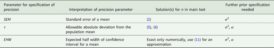
For α = 5% this amounts to the simple rule that SEM should be no larger than τ/2 or EHW/2. It also emerges that the precision measures τ and EHW are exchangeable from a practical point of view, even though they have somewhat different underlying rationales. We can also turn this around and first just compute the SEM for a given design to evaluate its precision. Then 2 × SEM is the allowable deviation τ or EHW the design permits to control. Because of the factors involved (1 for the SEM itself, and 2 for τ or EHW), we call this the 1-2 rule for a mean.
How to get a prior value for σ 2
General: The ideal is to find reports on similar studies as the one planned that report on the variance. Alternatively, a pilot study may be conducted to obtain a rough estimate of σ 2. Desirable though this may be, it is not always easy to get such information quickly.
A rule of thumb that may be useful here and does not make any distributional assumptions, is that the range in a sample of n observations, defined as the difference between the largest and smallest observed value in the sample, can be used to derive upper and lower bounds on the sample standard deviation $s = \sqrt {s^2}$ (van Belle, Reference van Belle2008, p. 36):

This rule is most useful in making quick assessments of problems in a given dataset, but it may also be useful in deriving a rough estimate of the standard deviation σ.
Normality: Welham et al. (Reference Welham, Gezan, Clark and Mead2015, p. 245) propose to approximate the standard deviation by:

where min and max are ‘the likely minimum and maximum value for experimental units receiving the same treatment’. The actual rationale of this equation stems from the normal assumption and the fact that 95% of the data are expected within two standard deviations from the mean. This means that for this approximation to work well, the data must have an approximate normal distribution, and min and max must be estimates of the 2.5 and 97.5% quantiles of the distribution. In other words, min and max must be the bounds of an interval covering about 95% of the expected data from experimental units receiving the same treatment.
Example 2: It is not easy to accurately guess the 2.5 and 97.5% quantiles. To illustrate the difficulty, consider random samples of different sizes n from a normal distribution. Of course, if such samples were available when planning an experiment, the sample variance could be computed directly and used in place of σ 2, and this would be the preferred thing to do. However, for the sake of illustrating the challenge with (14), imagine that we determine the observed minimum and maximum value in a sample of size n and plug these into the equation. Table 3 shows results for n = 4, 8, 15, 30, 50, 100. It is seen that with a sample size of n = 30 the expected range and median range come closest to the value of 4 that is postulated in (14). It emerges that a smaller sample size leads to under-estimation and a larger sample size to over-estimation of the standard deviation as per (14), if we simply plug in the observed minimum and maximum. But unless the sample size is very small, the approximation will be in the right ballpark, and that is usually sufficient for most practical purposes.
Table 3. Expected and median of range (maximum − minimum) for samples of different sample size n from standard normal distribution
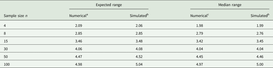
a Approximated as 2Φ−1(0.52641/n) (Chen and Tyler, Reference Chen and Tyler1999).
b Simulated based on 1000 runs, computing the mean in each run, and then taking the mean or median.
c Computed using the PROBMC function of SAS (Westfall et al., Reference Westfall, Tobias, Rom, Wolfinger and Hochberg1999, p. 45) as the 50% quantile of the studentized range distribution with infinite degrees of freedom.
Binary: Up to here, for the most part, we have assumed the normality of the response y. Often, the observed data are counts, and these are not normal. The simplest case is binary data, where the count is either 0 or 1. The response is then said to have a binary distribution, which has one parameter, the probability that the response is 1. This probability, in turn, is equal to the mean μ of the binary random variable. For this distribution the variance equals:

with 0 < μ < 1. Thus, to approximate the variance in this case, we need a guess of the mean μ. To be on the conservative side, we may consider the worst case with the largest variance σ 2, which occurs when μ = 0.5.
Example 3: A research institute conducts an opinion poll and considers the worst-case scenario that the proportion of voters favouring a particular party is μ = 0.5, in which case σ 2 = 0.25. The proportion of each party is to be estimated with precision SEM = 0.01. Thus, using (2), the sample size is chosen as:

Example 4: Monitoring foot pad health is an important task in rearing turkey. The prevalence of foot pad dermatitis in a given flock may be estimated by random sampling. Any animal with symptoms on at least one foot is considered as affected (Toppel et al., Reference Toppel, Spindler, Kaufmann, Gauly, Kemper and Andersson2019; for details on the scoring system see Hocking et al., Reference Hocking, Mayne, Else, French and Gatcliffe2008). Typical prevalences range around 0.5, so it is suitable to determine the sample size under the worst-case scenario μ = 0.5. If we set the allowable deviation from the true mean at τ = 0.1 with α = 5%, the sample size based on Eqn (6) is

Note that in using (6), we have assumed that the sample size n will be large enough for the central limit theorem to apply. We have further assumed that sampling is without replacement and that the population from which we are sampling is large relative to sample size (but see next sub-section entitled ‘Finite populations’).
Binomial: If on each experimental unit, we have m observational units, each with a binary response with the expected value μ (a proportion or probability), then the binomial distribution may be assumed, which has variance:

for the observed proportion y = c/m, where c is the binomial count based on the m observational units. Thus, to approximate the variance in this case, we also need a guess of the mean μ. Again, the worst-case scenario is μ = 0.5. In practice, the data may show over-dispersion relative to the binomial model. A simple way to model this is to assume variance:

where ϕ is an over-dispersion parameter (McCullagh and Nelder, Reference McCullagh and Nelder1989, p. 124). In this scenario, estimating the mean alone does not help in approximating the variance; we also need an estimate of the over-dispersion, and this puts us back to the general case, where independent prior information on the variance needs to be obtained.
Example 5: In a large potato field, n = 347 control points were distributed to assess the abundance of the potato weevil (Leptinotarsa decemlineata) (Trommer, Reference Trommer1986). At each control point, m = 20 potato plants where assessed for the presence or absence of the weevil. The counts of affected plants (c) per control point are reproduced in Table 4.
Table 4. Frequency distribution of the number of plants infested with the potato weevil (c) in samples of m = 20 plants at n = 347 control points (Trommer, Reference Trommer1986)

For each control plot, we can compute the observed proportion y = c/m. The sample mean of y across the n = 347 control points is $\bar{y}_ \bullet{ = } 0.2987$ , which is an estimate of the proportion μ of infested plants on the field. Under a binomial distribution, the variance of y would be estimated as ${{{\bar{y}}_ \bullet ( {1-{\bar{y}}_ \bullet } ) } / m} = 0.2987 \times\!$ ${0.7013} / {20} = 0.010474$
 . This is considerably smaller than the sample variance s 2 = 0.10788. From this, the overdispersion is estimated as $\hat{\phi } = {{s^2} / {[ {{{{\bar{y}}_ \bullet ( {1-{\bar{y}}_ \bullet } ) } / m}} ] }} = 10.2999$
 . This value corresponds to the one obtained from Pearson's chi-squared statistic for over-dispersed binomial data (McCullagh and Nelder, Reference McCullagh and Nelder1989, p. 127). Thus, the variance is about ten times the variance expected under a binomial model. The reason for this overdispersion is the clustering of patches of infested plants amidst areas of plants infested little or not at all, which is typical of crop diseases and pests. Incidentally, the hat symbol on ϕ indicates that this is the corresponding sample estimator of the parameter. We will subsequently use the hat notation in several places, also for other parameters. Further note that we could use $\hat{\mu }$
 and $\hat{\sigma }^2$
 in place of $\bar{y}_ \bullet$
 and s 2 to denote the sample mean and variance, respectively.
Now assume that we go to a new field and want to determine the number of control points (each with m = 20 plants) needed to achieve a half width of HW = 0.05 for a 95% confidence interval. A first rough assessment suggests that the infestation in the new field is in the order of μ = 0.1. The variance is σ 2 = ϕμ(1 − μ)/m = 10.299 × 0.1 × 0.9/20 = 0.04635. Using this in Eqn (11), we find:

Thus, n = 72 control points would be required to achieve this precision.
Poisson: Under the Poisson model for counts, the count y can take on any non-negative integer value (0, 1, 2,…). The variance of y is:

So again, a rough estimate of the mean is needed to approximate the variance. There is no worst-case scenario that helps as the variance increases monotonically with the mean μ. Moreover, it needs to be considered that there is often over-dispersion relative to the mean, so the variance is:

where ϕ is an over-dispersion parameter (McCullagh and Nelder, Reference McCullagh and Nelder1989, p. 198). As with the over-dispersed binomial distribution, in this scenario, estimating the mean alone does not help in approximating the variance; we also need an estimate of the over-dispersion, and this, yet again, puts us back to the general case.
It is stressed that exact methods should be used for small binomial sample sizes m and also for small means in case of the Poisson. These exact methods, which are somewhat more involved (see, e.g., Agresti and Coull, Reference Agresti and Coull1998; Chen and Chen, Reference Chen and Chen2014; Shan, Reference Shan2016), will not be considered here.
Example 6: Inoculum density of Cylindrocladium crotalariae was assessed on 96 quadrats in a peanut field. On each quadrat, the number of microsclerotia was counted (Hau, Campbell and Beute, Reference Hau, Campbell and Beute1982). The frequency distribution is given in Table 5.
Table 5. Frequency distribution of the number y of microsclerotia (Cylindrocladium crotalariae) per quadrat on n = 96 quadrats in a peanut field (Hau et al., Reference Hau, Campbell and Beute1982; Figure 3(b))

The mean count is $\bar{y}_ \bullet{ = } 7.990$ , whereas the sample variance is s 2 = 30.47, showing substantial over-dispersion. The overdispersion is estimated as $\hat{\phi } = {{s^2} / {{\bar{y}}_ \bullet }} = {{30.47} / {7.990}} = 3.841$
 . Again, this corresponds to the value obtained from Pearson's generalized chi-squared statistic (McCullagh and Nelder, Reference McCullagh and Nelder1989, p. 328). Now a new field is to be assessed on which first inspection by eyeballing suggests a mean infestation of μ = 20 microsclerotia per quadrat. We would like to estimate the population mean of the field with a precision of SEM = 2. The variance is expected to be σ 2 = ϕμ = 3.841 × 20 = 76.28. From Eqn (2) we find:

Thus, n = 20 quadrats are needed to achieve the targeted precision.
Finite populations
So far we have assumed that the population from which we are sampling (without replacement) is infinite, or very large. When the population is small, it is appropriate to consider a finite population correction, meaning that the VM equals (Kish, Reference Kish1965, p. 63):

where N is the population size. The methods for sample size determination in the previous sub-sections are applicable with this modification. Note that when n = N, i.e. under complete enumeration of the population, the variance in (20) reduces to zero as expected, because the finite population correction (N − n)(N − 1)−1 is zero in this case. For illustration, we consider the specification of an allowable absolute deviation τ of the sample mean from the population mean with probability α. Thus, we may equate ${{\tau ^2 } / {{\mathop{\rm var}} ( {{\bar{y}}_ \bullet } ) }} = z_{1-\alpha /2}^2$ as we have done in the previous sub-sections. Solving this for n using (20) yields:

Note that this is equal to (6) when N approaches infinity. Applying this to the binary case with σ 2 = μ(1 − μ) yields (Thompson, Reference Thompson2002, p. 41)

Example 3 (cont'd): In opinion polls, the population from which a sample is taken usually has size N in the order of several millions, which is huge compared to the customary sample sizes in the order of n = 2500. In this case, the finite population correction may safely be ignored.
Example 4 (cont'd): If the flock size is N = 4000 (Toppel et al., Reference Toppel, Spindler, Kaufmann, Gauly, Kemper and Andersson2019), and we use the same specifications as before, the sample size as per (22) is n = 94, down from n = 97 when the finite population correction is ignored (Eqn 6).
Comparing two means
In comparative studies and experiments, the objective is usually a pairwise comparison of means (Bailey, Reference Bailey2009). Thus, we are interested in estimating a difference δ = μ 1 − μ 2, where μ 1 and μ 2 are the means to be compared. Here, we consider the case where the observations of both groups are independent. In this case, the variance of a difference (VD) between two sample means $\bar{y}_{1 \bullet }$ and $\bar{y}_{2 \bullet }$
 equals ${\mathop{\rm var}} ( {{\bar{y}}_{1 \bullet }-{\bar{y}}_{2 \bullet }} ) = n_1^{{-}1} \sigma _1^2 + n_2^{{-}1} \sigma _2^2$
 , where n 1 and n 2 are the sample sizes and $\sigma _1^2$
 and $\sigma _2^2$
 are the variances in the two groups. If we assume homogeneity of variance, this simplifies to ${\mathop{\rm var}} ( {{\bar{y}}_{1 \bullet }-{\bar{y}}_{2 \bullet }} ) = ( {n_1^{{-}1} + n_2^{{-}1} } ) \sigma ^2$
 , where σ 2 is the common variance. Further, if the sample size is the same (n) in each group, which is the optimal allocation under homogeneity of variance, this further simplifies to ${\mathop{\rm var}} ( {{\bar{y}}_{1 \bullet }-{\bar{y}}_{2 \bullet }} ) = 2n^{{-}1}\sigma ^2$
 . Here, we make this assumption for simplicity. Note that the variance is just twice the variance of a sample mean. Thus, apart from this slight modification, all methods in the previous section can be applied without much further ado, so the exposition of these methods can be brief here.
Determining sample size based on a precision requirement
In this section, we assume approximate normality of the response or sufficient sample size for the central limit theorem to ensure approximate normality of treatment means.
Precision requirement specified in terms of the standard error of a difference
The standard error of a difference (SED) of two sample means equals:

Equation (23) may be solved for n to yield:

Example 7: Ross and Knodt (Reference Ross and Knodt1948) conducted a feeding experiment to assess the effect of supplemental vitamin A on the growth of Holstein heifers. There was a control group and a treatment group, both composed of 14 animals. The allocation of treatments to animals followed a completely randomized design. One of the response variables was weight gain (lb.). The pooled sample variance was s 2 = 2199 lb.2, and treatment means were in the order of 200 lb. Suppose a follow-up experiment is designed to compare the control to a new treatment with an improved formulation of the vitamin A supplementation with an SED of 20 lb. Setting σ 2 = 2199 lb.2 based on the prior experiment, the required sample size is

Precision requirement specified in terms of the allowable deviation of estimate of difference from its true parameter value
The sample size required per treatment to ensure with probability 1 − α that the deviation of the estimated difference from the true difference is no larger than $\tau _\delta$ is:
is:

For α is 5%, this is approximately:

Example 7 (cont'd): Suppose we are prepared to allow a deviation of $\tau _\delta = 20\,{\rm lb}$ . Thus, using σ 2 = 2199 we require:

This is four times the sample size required to achieve an SED of 20 lb. The precision achieved here is SED = 10 lb., which is half the desired $\tau _\delta$ .
.
Precision requirement specified in terms of the allowable half width of a confidence interval for a difference
A confidence interval for δ with (1 − α) × 100% coverage probability can be computed as:

where t w;1−α/2 is the (1 − α/2) × 100% quantile of the t-distribution with w = 2(n − 1) degrees of freedom and s 2 is the pooled sample variance, estimating the population variance σ 2. Again, the exact method to determine the sample size for the confidence interval of a difference requires numerical methods as implemented in software packages. Here, we consider an approximate method. The half width of the interval is $HW = t_{w; 1-\alpha /2}\sqrt {2s^2/n}$ . It is worth pointing out that this HW is equal to the least significant difference (LSD) for the same α as significance level, a point which we will come back to in the next section. The approximation replaces t w;1−α/2 with z 1−α/2 and s 2 with σ 2, yielding a expected half width (EHW) of

which we may also regard as the expected LSD (ELSD). Then solving for n yields:

This equation is seen to be equivalent to (25) when replacing $\tau _\delta$ with EHW. This approximate solution will tend to yield somewhat smaller sample sizes than the exact numerical solution.
Example 7 (cont'd): Suppose we want to achieve EHW = 20 lb. with α = 5%. This requires:

which is the same sample size as requires to achieve an allowable deviation of $\tau _\delta = 20\,\;{\rm lb}.$ , and also leads to SED = 10 lb., half the desired EHW.
Precision requirement specified in terms of difference to be detected by a t-test
A t-test may be used to test the null hypothesis H 0: δ = 0 against the alternative H A: δ ≠ 0. The t-statistic for this test is:

This has a central t-distribution on w = 2(n − 1) degrees of freedom under H 0: δ = 0 and a non-central t-distribution under the alternative H A: δ ≠ 0. There are two error rates to consider with a significance test, i.e. α, the probability to falsely reject H 0 when it is true, and β, the probability to erroneously accept H 0 when it is false. The complement of the latter, 1 − β, is the power of the test, i.e., the probability to correctly reject H 0 when it is false. To plan sample size, we need to make a choice for the desired values of both α and β. Moreover, prior information on the variance σ 2 is needed, as well as a specification of the smallest relevant value of the difference δ that we want to be able to detect with the test. These choices then determine the required sample size. Again, an exact solution for n requires numerical integration using the central t-distribution under H 0 and the non-central t-distribution under HA (Welham et al., Reference Welham, Gezan, Clark and Mead2015, p. 248). Some authors approximate the non-central t-distribution with the central one (Cochran and Cox, Reference Cochran and Cox1957, p. 20; Bailey, Reference Bailey2009, p. 36). A more portable approximate solution that replaces the central and non-central t-distributions with the standard normal, and the sample variance s 2 with the population variance σ 2, is obtained as (van Belle, Reference van Belle2008, p. 30):

where z 1−α/2 is as defined before and z 1−β is the (1 − β) × 100% quantile of the standard normal distribution. This equation is easily derived by observing that under H 0, t is approximately standard normal, with the critical value for rejection at ±z 1−α/2, the (1 − α/2) × 100% quantile of the standard normal. Under HA, t is approximately normal with unit variance and mean δ/SED, with SED depending on n as shown in (23). This distribution has its β × 100%-quantile at δ/SED − z 1−β. These two quantiles under the H 0 and HA distributions must match exactly for the desired α and β, so we can equate them and solve for n, yielding Eqn (31).
A conventional value of α is 5%, but 1% or 10% are also sometimes used. Typical choices for β are 5%, 10% and 20%. For routine application, it is convenient to define C α,β = (z 1−α/2 + z 1−β)2 and compute this for typical choices of α and β (Table 6). These values of C α,β can then be used in the equation:

Table 6. Values of C α,β = (z 1−α/2 + z 1−β)2 for typical choices of α and β

A portable version of (32) for the very common choice α = 5% and β = 10% is:

Other portable equations can of course be derived for other desired values of α and β. It is instructive to compare Eqn (33) for the t-test with the precision-based Eqn (26). Importantly, unless the power we desire is small, (33) yields a considerably larger sample size when we use the same values for the difference to be detected (δ) in (33) and the allowable deviation of the estimated from the true difference $( {\tau_\delta } )$ in (26). As we have explained, the latter can also be equated to the desired ELSD. Specifically, this means that choosing sample size so that a desired value for $\tau _\delta$
 or ELSD is achieved does not at all ensure sufficient power (1 − β) to detect a critical difference δ of the same size. In fact, if δ = ELSD, the t-test has an expected power of 50% only, which will hardly be considered satisfactory. We will need an ELSD substantially smaller than $\tau _\delta$
 to achieve a reasonable power. For our portable example with a power of 90%, the ratio of required ELSD over δ can be approximated by dividing (33) by (26) and solving for the ratio:

It may also be noted that if the desired power indeed equalled 50%, we would have z 1−β = z 0.5 = 0, in which case (31) takes the same form as (25). So in this special case of a power of 50%, we may say that the specification of a value for δ in (31) is equivalent to specifying the same value for $\tau _\delta$ (equivalent to ELSD) in (25). This coincidence is of little practical use, however, because a power of 50% is rarely considered sufficient. The more important point here is that in all other cases, specifying the same value for δ in (31) and for $\tau _\delta$
 in (25) does not lead to the same sample size.
Example 7 (cont'd): A difference of δ = 20 lb. is to be detected at α = 5% with a power of 90%. This can be achieved with an approximate sample size of:

As expected, this sample size is larger still than when we required EHW = 20 lb. or $\tau _\delta = 20\;\,{\rm lb}.$ . The precision attained here is better as well, amounting to SED ≈ 6 lb.
We also use this example to assess the degree of the approximation involved by replacing the central and non-central t-distributions with the standard normal in (31). For the case at hand, the exact result (obtained with PROC POWER in SAS) yields n = 117, which is very close to the approximate result of n = 116. To explore this further, we also did the exact and approximate calculations for a range of larger values of the relevant difference δ. The results in Table 7 show that the approximation is very good, even when the exact sample size is as small as n = 3. It emerges that if one wants to be on the safe side, adding one or two to the approximate sample size per group should suffice.
Table 7. Required sample size for unpaired t-test at α = 5% with a power of 90% for σ 2 = 2199 lb.2 and a range of values for the smallest relevant difference δ in lb
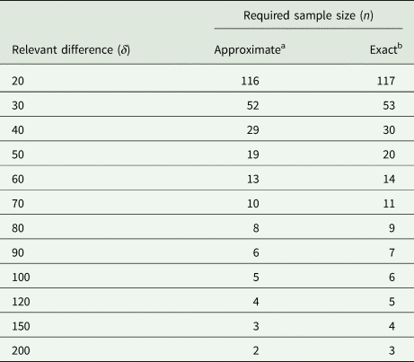
a Using Eqn (31).
b Using PROC POWER of SAS.
The equations considered so far require specifying the difference to be detected (δ) in absolute terms. It is sometimes easier for researchers to specify this in relative terms instead, i.e., as a proportion or percentage difference. For this purpose, Eqn (31) can be slightly rewritten. To do so, we define the relative difference as:

where μ = (μ 1 + μ 2)/2 is the overall mean. The standard deviation can also be expressed in relative terms, and this is known as the coefficient of variation, CV = σ/μ. With these definition, Eqn (31) can be rearranged to yield the approximation:

The portable version of (35) for the very common choice α = 5% and β = 10% is (see Table 6):

These equations work equally with δ r and CV expressed as proportions or as percentages.
Example 7 (cont'd): The means for the control and treatment groups were 187.6 and 235.9 lb. From this, the coefficient of variation is computed as CV = 22.15% = 0.2215. Suppose that in a new experiment we want to be able to detect a relative treatment difference of δ r = 10% = 0.1 compared to the overall mean at α = 5% with a power of 90%. Here we need a sample size of:

Example 8: Four traits are to be assessed to compare two different milking methods, i.e. a milking robot and a milking parlour. Long-term records on these four traits are available from 142 cows of the same population from which the animals for the experiments are to be drawn and allocated to the two treatments at random. Sample means and variances are reported in Table 1. Discussions with the animal scientists conducting this experiment identified the smallest relevant differences δ for the four traits as shown in Table 1. Based on these specifications, the sample size n per treatment for an unpaired t-test for α = 5% and a power of 85% were determined using Eqn (32) for each trait. It is seen that the sample size differs between traits, illustrating that when an experiment involves several traits, a compromise must be struck regarding a common sample size. We also note that the SED achieved with these sample sizes is about 1/3 of the smallest relevant difference δ for each trait, a point we will take up again in the next section.
We note in passing that it is quite common to express effect size not relative to a mean but relative to the standard deviation (d = δ/σ; Cohen, Reference Cohen1977, Reference Cohen1992), a measure also known as Cohen's d, but agree with Lenth (Reference Lenth2001) that it is difficult, if not misleading, to think about effect size in these terms.
Summary and the 1-2-3 rule
We can summarize the procedures under the four types of specification in this section so far as shown in Table 8. It is instructive at this point to highlight that all procedures involve the SED. This important fact can be exploited to convert all procedures into simple rules in terms of the choice of SED. Thus, for achieving a desired value of $\tau _\delta$ , EHW or ELSD, we need to choose:

Table 8. Overview of procedures for determining sample size for a mean difference

It is also seen that in practice, the three precision measures $\tau _\delta$ , EHW or ELSD are exchangeable, despite differences in their derivation. For detecting a minimal effect size δ, we need to choose:

This latter fact led Mead (Reference Mead1988, p. 126; also see Mead et al., Reference Mead, Gilmour and Mead2012, p. 137) to suggest the rule of thumb that SED should be no larger than |δ|/3, corresponding to an approximate power of 1 − β = 0.85 at α = 5% because z 1−α/2 + z 1−β ≈ 3. By comparison, using z 1−α/2 ≈ 2 for α = 5% in Eqn (37) yields the rule that SED should be no larger than $\tau _\delta /2 = EHW/2 = ELSD/2$ . As in the case of a single mean (previous section), we can turn this around and first compute the SED for a given design to evaluate its precision. Then 2 × SED is the allowable deviation $\tau _\delta$
 (EHW, ELSD) the design permits to control. Similarly, 3 × SED is the smallest absolute difference |δ| the design can detect. Because of the divisors and multipliers involved (1 for SED itself, 2 for τδ, EHW or ELSD, and 3 for δ), we refer to this set of portable equations and rules as the 1-2-3 rule for a difference.
Procedures for counts
As was already pointed out in the previous sub-section, the common distributional models for counts (e.g., binary, binomial, Poisson) imply that the variance depends on the mean. When it comes to the comparison of means between two groups, the consequence is that there is the heterogeneity of variance between the groups unless the means are identical. Therefore, all specifications for sample size need to be made explicitly in terms of the two means, and not just their difference, which is a slight complication compared to the normal case assuming homogeneity. As a result of this slight complication, there are several approximate approaches for determining the sample size. Most of them rely on the approximate normality of estimators of the parameters, which is a consequence of the central limit theorem. This is not the place to give a full account of all the different options. Many of these are nicely summarized in van Belle (Reference van Belle2008).
Here, we will just mention one particularly handy approximate approach that employs a variance-stabilizing transformation of the response variable y. For the Poisson distribution with large mean, the square root transformation $z = \sqrt y$ stabilizes the variance at ${\mathop{\rm var}} ( z ) \approx {1 / 4}$
 (McCullagh and Nelder, Reference McCullagh and Nelder1989, p. 196). For the binomial distribution with large m (number of observational units per sample), the angular transformation $z = \arcsin \{ {{( {{c / m}} ) }^{{1 / 2}}} \}$
 , where c is the binomial count, approximately stabilizes the variance at ${\mathop{\rm var}} ( z ) \approx {1 / {( {4m} ) }}$
 (McCullagh and Nelder, Reference McCullagh and Nelder1989, p. 137). Allowing for over-dispersion, which is the rule rather than the exception in comparative experiments in agriculture (Young et al., Reference Young, Campbell and Capuano1999), the variance needs to be adjusted to ${\mathop{\rm var}} ( z ) \approx {\phi / 4}$
 and ${\mathop{\rm var}} ( z ) \approx {\phi / {( {4m} ) }}$
 for the Poisson and binomial distributions, respectively. The advantage of using these variances on the transformed scale is that they are independent of the mean, simplifying the sample size calculation a bit. Thus, we can use:

for the over-dispersed Poisson and:

for the over-dispersed binomial distribution in equations in the preceding sub-sections. At the same time, however, the specifications for $\tau _\delta$ and δ need to be made on the transformed scale, and this, in turn, requires that the two means need to be specified explicitly, rather than just their difference. For example, under the (over-dispersed) Poisson model we use:

and under the (over-dispersed) binomial model we use:

where the means correspond to the binomial probabilities being compared (Cohen, Reference Cohen1977, p. 181, Reference Cohen1992). These expressions can be inserted in Eqns (31)–(33), leading to explicit equations for the Poisson and binomial models if desired (Cochran and Cox, Reference Cochran and Cox1957, p. 27; van Belle, Reference van Belle2008, p. 40 and p. 44). With over-dispersion, which should be the default assumption for replicated experiments, a prior estimate of the over-dispersion parameter ϕ will be required to evaluate the variances in (39) and (40) for use in the expressions in the preceding sub-sections. Such an estimate can be obtained via Pearson's chi-squared statistic or the residual deviance based on a generalized linear model (GLM; McCullagh and Nelder, Reference McCullagh and Nelder1989). Later in this paper, we will consider a simulation-based approach that can be applied for count data when the simplifying assumptions made here (e.g., large binomial m or large Poisson mean) are not met. Also, we note in passing that the angular transformation, originally proposed for binomial proportions, may sometimes work for estimated (continuous) proportions, but see Warton and Hui (Reference Warton and Hui2011) for important cautionary notes, Piepho (Reference Piepho2003) and Malik and Piepho (Reference Malik and Piepho2016) for alternative transformations, and Duoma and Weedon (Reference Duoma and Weedon2018) on beta regression as an alternative.
Example 9: A field experiment is to be conducted in randomized complete blocks to compare a new herbicide against the weed gras Bromus sterilis to a control treatment. The number of weed plants per m 2 will be assessed by sampling five squares of 0.25 m2 per plot and dividing the total count of weed plants by 1.25 m2. A previous trial with the same kind of design yielded the total counts per plot shown in Table 9. Analysis of this trial using a GLM for overdispersed Poisson data using a log-link (McCullagh and Nelder, Reference McCullagh and Nelder1989) yielded the overdispersion estimate $\hat{\phi } = 2.59$ . For the future trial, the smallest relevant effect is specified in terms of the mean μ 1 = 15 plants per 1.25 m2 for the control and the mean μ 2 = 3 plants per 1.25 m2 for a new herbicide, corresponding to a reduction of weed infestation by 80%. Using a square-root transformation with variance in (39) and effect size in (41), we find from (31) for α = 5% and a power of 90% that $\delta = \sqrt {15} -\sqrt 3 = 2.14$
 , σ 2 = 2.59/4 = 0.648 and:

Table 9. Total counts of Bromus sterilis on 1.25 m2 per plot in an experiment laid out as a randomized complete block design with four treatments and four blocks (Büchse and Piepho, Reference Büchse and Piepho2006)
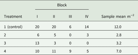
Incidentally, the variance specification based on a GLM (σ 2 = 0.648) is quite close to the estimate by an analysis of the square-root transformed counts (s 2 = 0.607), confirming the utility of the simple data transformation approach. It may be added that this sample size is smaller than the one actually used (n = 4). That sample size, however, would not have been sufficient to detect a weed reduction by 50% at the same level of significance and power.
Example 10: A field experiment is to be conducted to assess the effect of a neonicotinoid on the abundance of an insect species. The expected abundance for the control is in the order of ten individuals per trap. The smallest relevant difference for the treatment corresponds to a 25% drop in abundance, amounting to 7.5 individuals per trap for the treatment. We set μ 1 = 10, μ 2 = 7.5, α = 5% and β = 20%. Assuming a Poisson distribution, we initially set σ 2 = 0.25 as per (39) on the optimistic assumption of no overdispersion. We find $\delta = \sqrt {\mu _1} -\sqrt {\mu _2} = 0.4237$ and use all of these specifications in Eqn (31), finding n = 21.86 ⇒ 22. From a previous study, we expect an overdispersion of ϕ = 1.3. Hence, we adjust our sample size upwards to n = ϕ × 21.86 = 1.3 × 21.86 = 28.42 ⇒ n = 29.
Example 11: Diseases or traits due to hereditary defects can often be detected by gene tests which require a population-wide evaluation. The principal idea is to test for an association between the status of a gene (which may have three outcomes/genotypes in a diploid organism) and the occurrence of a disease. For instance, being horned or hornless in cattle is caused by a mutation at the ‘polled locus’, and a gene test has already been established to increase the frequency of polled cattle in future through selective mating. To test whether the horned or hornless phenotype in cattle is caused by a specific variant in the genome, we distinguish factor level A (genotype pp) and B (genotype Pp or PP) and consider the 2 × 2 classification in Table 10.
Table 10. Expected counts in a 2 × 2 classification of groups and treatments

The parameters μ 1 and μ 2 are the probabilities of occurrence of level A in the two groups, and n 1 and n 2 are the sample sizes for the two groups.
The task is to approximate sample size allowing the detection of differences in probabilities μ 1 and μ 2 between groups. Table 10 reflects the expected counts and an obvious solution is to continue with the binomial model using, e.g., μ 1 = 0.9 and μ 2 = 0.5 in Eqn (42) and σ 2 = 1/4. Using σ 2 = 1/4 instead of 1/(4m), as you would expect from the binomial model, is justified by treating the binary variable as a limiting case here (see Paulson and Wallis, Reference Paulson, Wallis, Eisenhart, Hastay and Wallis1947; cited in Cochran and Cox, Reference Cochran and Cox1957, p. 27; also see the Appendix). Assuming a balanced design and δ = 0.4637 from (42), yields n 1 = n 2 = n = 25 using Eqn (31) with α = 5% and a power of 90% (also see Cochran and Cox, Reference Cochran and Cox1957, p. 27). Using a more specifically tailored formula due to Fleiss (Reference Fleiss1981; also see eq. 2.50 in Rasch et al., Reference Rasch, Pilz, Gebhardt and Verdooren2011) yields n 1 = n 2 = 26, and further using a correction due to Casagrande et al. (Reference Casagrande, Pike and Smith1978; also see eq. 2.51 in Rasch et al., Reference Rasch, Pilz, Gebhardt and Verdooren2011, p. 49) yields n 1 = n 2 = 30, so our approximate approach lands us in the right ballpark. We conclude by noting that the task above could also be tackled with a chi-square test of independence on 1 degree of freedom or by a test of the log-odds ratio, as will be discussed later.
Paired samples
This section so far focused on unpaired, i.e. independent samples. When paired samples are considered, we may resort to procedures for a single mean, replacing the observed values y j with observed paired differences d j between two treatments or conditions. Accordingly, mean and variance of y j need to be replaced by mean and variance of paired differences d j. Because of this one-to-one relation with the case of a single mean, procedures for paired samples are slightly simpler than for unpaired samples. We note that the section for a single mean does not explicitly consider significance tests, but the confidence interval for a difference may be used to conduct a significance test of H 0 that the expected difference equals zero, exploiting the close relation between both procedures. The H 0 is rejected at the significance level α when the (1 − α) × 100% confidence interval for the difference does not include zero. Thus, all options can be implemented with the procedures for a single mean. As regards significance testing, Eqn (31) needs to be modified as:

where $\sigma _d^2$ is the variance of pairwise differences dj and approximate normality is assumed.
Example 12: An experiment was conducted with Fleckvieh dairy cows to compare the lying time per day indoors and outdoors on an experimental farm (Benz et al., Reference Benz, Kaess, Wattendorf-Moser and Hubert2020). Sufficient lying time is an important trait for claw health. A total of 13 cows, sampled randomly from the current population at the farm (~50 animals), were included in the experiment and their average lying time per day assessed in both phases using pedometers (Table 11). The indoor phase in the barn took place in early September 2017 and the outdoor phase was conducted in late September 2017.
Table 11. Lying times (min day−1) of 13 cows indoors and outdoors

From these data, the variance $\sigma _d^2$ of the 13 pairwise differences (d 1 = 745 − 614 = 113, etc.) is estimated at $s_d^2 = 7355$
 . If for a new study we want to be able to detect a lying time difference of δ = 40 min day−1 at α = 5% with a power of 80%, the required sample size is:

Thus, we would require 28 cows. This sample size is expected to yield SED = 14.29 (Eqn 1) and $EHW = \tau _\delta = 28.01$ (Eqns 6 and 10).
It is noted that the size of the population at the farm from which the cows are to be sampled, is relatively small. One might therefore consider a finite-sample correction to account for this as in described in the previous section for a single mean, which would lead to a slightly smaller sample size, but would restrict the validity of the results to the farm population studied. An alternative view is that the ~50 animals at the farm are themselves a sample from the much larger Fleckvieh population and that the objective of the study is not to characterize the limited population at the farm, but to characterize conditions at the farm itself. In this view, which provides a somewhat broader inference, it makes sense to regard the n = 28 animals as a sample from the broader Fleckvieh population, raised under the conditions of the farm at hand. In this case, a finite-population correction is not needed.
More advanced settings
More than two means
When more than two means are to be compared, the same methods as in the previous section can be used, as in the end we usually want to compare all pairs of means. The only additional consideration is that there may be a need to control the family-wise Type I error rate in case of multiple pairwise tests. In case of normal data, this means using Tukey's test rather than the t-test (Bretz et al., Reference Bretz, Hothorn and Westfall2011), and sample size calculations may be adjusted accordingly (Horn and Vollandt, Reference Horn and Vollandt1995; Hsu, Reference Hsu1996). A simple approximation is afforded by the Bonferroni method which prescribes dividing the targeted family-wise α by the number of tests. That number equals v(v − 1)/2 for all pairwise comparisons among v treatments, so the t-tests would be conducted at significance level α′ = α/[v(v − 1)/2]. In a similar vein, the Tukey or Bonferroni methods can also be used when considering confidence intervals desired to have joint coverage probability of (1 − α) × 100%; with the Bonferroni method this is achieved by computing (1 − α′) × 100% confidence intervals using the method in the previous section for the individual comparisons.
We note here that pairwise comparison of means are usually preceded by a one-way analysis of variance (ANOVA) F-test of the global null hypothesis of no treatment differences (though this is not strictly necessary when pairwise comparisons are done controlling the family-wise Type I error rate). It is also possible to determine sample size based on the power of the one-way ANOVA F-test (Dufner et al., Reference Dufner, Jensen and Schumacher1992, p. 196; Dean and Voss, Reference Dean and Voss1999, p. 49f.; Rasch et al., Reference Rasch, Pilz, Gebhardt and Verdooren2011, p. 59), and we will come back to this option in the next section. It is emphasized here that we think the consideration of pairwise comparisons is usually preferable for determining sample size also when v > 2, because it is more intuitive and easier in terms of the specification of the precision required. When the focus is on individual pairwise mean differences, all equations for unpaired samples remain valid with the variance σ 2 for the design in question. Specifically, these equations can be applied with the three most common and basic experimental designs used in agricultural research, i.e. the completely randomized design, the randomized complete block design, and the Latin square design (Cochran and Cox, Reference Cochran and Cox1957; Dean and Voss, Reference Dean and Voss1999).
Example 7 (cont'd): Suppose we want to add three further new formulations with vitamin A, increasing the total number of treatments to v = 5. If the specifications for the required precision or power remain unchanged, so does the required sample size per treatment group. Only the total sample size increases from 2n to vn = 5n. If we want to cater for a control of the family-wise Type I error rate at the α = 5% level, we may consider a Bonferroni approximation of the Tukey test and use a pairwise t-tests at α′ = α/[v(v − 1)/2] = 5%/[5 × 4/2] = 0.5%. Thus, we would replace z 1−α/2 with $z_{1-{\alpha }^{\prime}/2}$ , which for α′ = 0.5% equals $z_{1-{\alpha }^{\prime}/2} = 2.81$
 , compared to z 1−α/2 = 1.96 for α = 5%. Thus, sample size requirement according to (31) for δ = 20 lb. at α = 5% with a power of 90% would increase from n = 115 to n = 184 per group.
Regression models
The simplest case in regression is a linear regression of a response y on a single regressor variable x. Apart from sample size, the placement of the treatments on the x-axis needs to be decided. For a linear regression, the optimal allocation is to place half the observation at the lower end, xL, and the other half at the upper end, xU, of the relevant range for x (Rasch et al., Reference Rasch, Herrendörfer, Bock, Victor and Guiard1998, p. 273; Rasch et al., Reference Rasch, Pilz, Gebhardt and Verdooren2011, p. 127f.). Optimal allocation for higher-order polynomials or intrinsically nonlinear models is more complex and will not be elaborated here (see, e.g., Dette, Reference Dette1995). But it is stressed that the optimal allocation for such models will almost invariably involve more than two x-levels.
The simplest linear case, however, can be used to make a rough assessment of the required sample size. The optimal design with observations split between xL and xU essentially means that at both points the mean needs to be estimated. If we denote these means by μ L and μ U, the linear slope is given by γ = (μ U − μ L)/(x U − x L), showing that estimating the slope is indeed equivalent to comparing the two means. This, in turn, suggests that we can use the methods in Section ‘Comparing two means' to determine the sample size. We just need to quantify the relevant change in the response from xL to xU, given by δ = μ U − μ L.
With many nonlinear models, more than two x-levels will be needed, and the definition of a relative effect may be more difficult. Often, parts of the expected linear response can be well approximated by linear regression, and relevant changes defined by parts. Therefore, consideration of the simplest linear case may be sufficient to determine a suitable number of observations per x-level. It may also be considered that higher-order polynomials (quadratic or cubic) can be estimated based on orthogonal polynomial contrasts (Dean and Voss, Reference Dean and Voss1999, p. 261), which also constitute a type of mean comparison, giving further support to our portable approach.
Our considerations here do not imply that we would normally recommend doing a linear regression with just two x-levels, unless one is absolutely sure that the functional relationship will indeed be linear. In order to be able to test the lack-of-fit of any regression model (Dean and Voss, Reference Dean and Voss1999, p. 249; Piepho and Edmondson, Reference Piepho and Edmondson2018), one or two extra x-levels will be needed. Also, for each parameter in a nonlinear regression model to be estimated, one additional x-level will be required. This leads to the following rule-of-thumb for the number of x-levels: (i) Determine the number of parameters of the most complex nonlinear model you are intending to fit (there may be several). (ii) That number plus one or two should be the number of x-levels in the experiment. The number of replications per x-level can then be determined as in the previous section. More sophisticated approaches for allocating samples to x-levels are, of course, possible, especially when several x-variables are considered, and these may involve unequal sample sizes between x-levels (Box and Draper, Reference Box and Draper2007). Also, the x-levels are usually equally spaced, even though depending on the assumed model unequal spacing may sometimes be preferable (Huang et al., Reference Huang, Gilmour, Mylona and Goos2020). These more sophisticated approaches are not considered here, however, because they are less portable.
Continuing with the idea that a rough assessment of sample size is possible by considering the linear case and the comparison of the response at xL and xU, and keeping in mind that usually we want to test more than just the two extreme levels xL and xU, we may consider the case of v treatments equally spaced on the x-axis. Generally, the variance of the estimate of the linear slope γ equals σ 2, divided by the sum of squares of the x-levels. If we assume that the v x-levels x 1, x 2, …, xv are equally spaced and each level is replicated n times, the standard error of a slope (SES) equals:

where D v = [12(v − 1)2]/[v(v 2 − 1)]. Values of Dv for typical values of v are given in Table 12. An interesting limiting case occurs when v = 2, for which Dv = 2. If, without loss of generality, we assume xL = 0 and xU = 1, then SES equals SED in (23), confirming our suggestion that considering a comparison of the means at xL and xU provides a useful rough guide to sample size per treatment level for linear regression. Further considering (44) and the values of Dv for v > 2 in Table 12 confirms that this provides a conservative estimate of sample size. Solving (44) for n yields the sample size per treatment required to achieve a preset value of SES:

Table 12. Values of Dv (see near Eqn 44) for v = 2, 3, …, 8 treatment levels

Similar derivations give the equations based on the allowable deviation of the estimate of γ from its true value, $\tau _\gamma$ , as:
, as:

and based on the EHW as:

Finally, the sample size based on a t-test of H 0: γ = 0 v. H A: γ ≠ 0 is:

where γ is the smallest absolute value of the slope that we consider relevant. By way of analogy to procedures in the two previous sections (1-2 and 1-2-3 rules), all of these rules could be converted into specifications in terms of the required SES, but this is not detailed here for brevity.
Example 7 (cont'd): In the experiment conducted by Ross and Knodt (Reference Ross and Knodt1948), the basal ratio contained 114 000 USP units of vitamin A per daily allowance per heifer (USP is a unit used in the United States to measure the mass of a vitamin or drug based on its expected biological effects). This was supplemented with 129 400 USP units of vitamin A for the 14 heifers in the vitamin A group. Now assume a follow-up experiment is planned in which v = 5 equally spaced levels of supplementation between xL = 0 and xU = 129 400 USP units are to be tested. We use σ 2 = 2199 as before. When illustrating Eqn (31) for a t-test to compare two means, we had considered the difference of δ = 20 lb to be the smallest relevant effect size. In our regression, this increase corresponds to a linear slope of γ = (μ U − μ L)/(x U − x L) = δ/129 400 = 20/129 400. Also note that γ(x U − x L) = δ = 20 lb. Hence, using (48) the sample size needed per treatment for linear regression with v = 5 levels at α = 5% with a power of 90% is:

This is somewhat smaller than the sample size needed per treatment for comparing two means, where we found n = 116. The ratio of these two sample sizes, 93/116 ≈ 0.8, equals the ratio of the values for Dv for v = 5 and v = 2 (Table 12), 1.60/2.00 = 0.8, which is no coincidence. The example confirms our assertion that sample size based on comparing two means provides a rough guide to sample size for linear regression based on more than two x-levels.
Pseudoreplication
The number of replications in a randomized trial is given by the number of experimental units to which treatment is independently and randomly allocated. In a field trial, the experimental unit is the plot. In some cases, there may be multiple observations per experimental unit so the number of observational units exceeds that of experimental units. It is generally important to bear in mind that observational units and experimental units do not necessarily coincide (Bailey, Reference Bailey2009). If there are multiple observations per experimental unit, these are denoted as sub-samples (Piepho, Reference Piepho1997; Welham et al., Reference Welham, Gezan, Clark and Mead2015, p. 47) or pseudo-replications (Hurlbert, Reference Hurlbert1984; Davies and Gray, Reference Davies and Gray2015).
There are two ways to properly analyse such data: (i) Compute means per experimental unit and then subject these to ANOVA in accordance with the randomization layout. (ii) Fit a mixed model in accordance with the randomization layout that has two random effects, one for experimental units and one for observational units. In case the number of observations per experimental unit is constant, both analyses will yield identical results, unless the variance for experimental units is estimated to be zero under option (ii), in which case option (i) is preferable for better Type I error control. With an unequal number of observations per experimental unit, option (ii) is to be preferred because it gives proper weights to experimental units depending on the respective number of observational units (Piepho, Reference Piepho1997). In this section, we will restrict attention to the equi-replicated case, which is also preferable in terms of overall precision.
The sample size here has two components, i.e., the number of experimental units (n e) and the number of observational units per experimental unit (n o). The latter number may be a given, depending on the circumstances. Where n o can be freely chosen, its optimal value depends on the variance components for two sources of variation, i.e. the variance between experimental units ($\sigma _e^2$ ) and the variance between observational units within the same experimental unit ($\sigma _o^2$
 ). A linear model (LM) for the jth observation on the ith experimental unit (yij) can be written as:

where ei is the error of the ith experimental unit, having variance $\sigma _e^2$ , and oij is the observational error of yij, having variance $\sigma _o^2$
 . The variance of a mean (VM) is:

where $\bar{y}_{ {\bullet}{\bullet} } = ( {n_en_o} ) ^{{-}1}\sum\nolimits_{i = 1}^{n_e} {\sum\nolimits_{j = 1}^{n_o} {y_{ij}} }$ is the mean. This equation shows that increasing n e reduces the impact of both $\sigma _e^2$
 and $\sigma _o^2$
 , whereas increasing n o only reduces the impact of $\sigma _o^2$
 . Hence, an additional experimental unit is worth more than an additional observational unit. If c e is the operational cost for one experimental unit and c o is the cost for one observational unit, both measured in the same units (e.g., in monetary terms or as working time), the optimal number of observational units per experimental unit is given by (Snedecor and Cochran, Reference Snedecor and Cochran1989, p. 448):

For given sample size n e, this minimizes the total cost C = n ec e + n en oc o. Once the optimal n o is determined, the required n e can be determined using the methods in the previous two sections (single mean, two means), setting n e = n and

We also note that for completely randomized designs or randomized complete block designs or Latin square designs, the variance of a difference (VD) will be VD = 2 × VM and the standard error of a difference will be $SED = \sqrt {VD} = \sqrt 2 \times SEM$ , where $SEM = \sqrt {VM}$
 .
.
Example 13: A trial was conducted to assess the merit of four different intermediate crops following the main crop oats. The crops were tested with three different sowing methods, allocated to main plots in four complete blocks. The five different intermediate crops were allocated to the subplots. Cover by these intermediate crops was assessed based on five randomly placed counting frames (0.1 m2 each) per plot. One of the traits was the visually estimated percentage of ground cover by the intermediate crop. Inspection of the residuals indicated that an angular transformation would stabilize the variance. For the transformed data, the variance for the main plots was estimated to be zero. The variance for subplots was 0.000318 and that for samples within subplots was 0.00840.
For a future trial of the same kind, to be laid out as a randomized complete block design, the optimal number of samples per plot (no) is to be determined. For this purpose, we use values $\sigma _e^2 = 0.000318$ and $\sigma _o^2 = 0.00840$
 , showing that the within-plot variance dominates. Cost for plots and samples are not quantified here. Instead, we try different feasible values for no as shown in Table 13 and compute the associated value of σ 2 as per (52). With these variances, we determine the optimal sample size ne using Eqn (31) with α = 5% and β = 20%. As we used a data transformation, specification of δ is based on Eqn (42), where μ 1 and μ 2 are coverages, expressed as proportions, reflecting the smallest relevant difference at expected orders of magnitude for both proportions. Here, we set μ 1 = 0.1 and μ 2 = 0.2.
Table 13. Number of plots (ne) required as depending on number of samples per plot (no) for α = 5%, β = 20%, μ 1 = 0.1 and μ 2 = 0.2 based on angular transformation for intermediate crop experiment (Example 13)

If we use two samples per plot, we need four replicates. If we use only a single sample per plot, seven replicates are needed. Conversely, we may conclude that for a given trial with four replicates, a sample size of no = 5 as used in the current trial is more than required at the pre-specified level of power.
Example 14: In a field experiment with spring barley, the number of ears per two metres within rows is to be determined at the start of ripening (BBCH stage 83; Bleiholder et al., Reference Bleiholder, van den Boom, Langelüddecke and Stauss1989). The experiment has eight treatments and ne = 4 replications, arranged in complete blocks. The number of ears is determined by sampling sections of two metre length within rows. A decision needs to be taken on the spot as to the number no of sections to be sampled per plot. To this end, initially two sections are sampled per plot and the data analysed to estimate the variance components for plots and sections within plots. The data is given in Table 14. The response is a count but inspection of residual plots (Kozak and Piepho, Reference Kozak and Piepho2018) indicated no serious departure from the homogeneity of variance assumption. Thus, the untransformed data were analysed using a linear mixed model (LMM) with fixed effect for treatments and replicates and random effects for plots and sections (residual effect). The resulting variance component estimates, obtained using a mixed model package on a laptop computer during the coffee break, are $\hat{\sigma }_e^2 = 12.00$ and $\hat{\sigma }_o^2 = 19.98$
 . These estimates are now used to plan the final sample size no for a t-test using Eqn (31). Observing that the plot mean has the variance given in (52), we plug this equation into (31). Solving for no yields:

Table 14. Number of ears per section within rows (2 metres) (Example 14)

It is important to note that this equation can return a negative value for no. If this happens, the number of replications (ne), which is a fixed quantity for an ongoing field experiment, is too small to achieve the desired precision. By way of illustration, assume that we want to plan for a t-test at α = 5%, a power of 90% and a relevant difference of δ = 5 ears per section. The resulting approximate sample size is:

A negative sample size is not feasible, of course. It can be shown algebraically that the reason for this result is that ne = 4 are too few replications to achieve the required precision; even a very large number of sections (no) would not achieve this, because as per Eqn (52) the variance $\sigma ^2\approx \sigma _e^2 = 12.00$ , which is too large. In the next experiment of this kind, it will therefore be prudent to increase the number of replications (ne). To illustrate further, consider the less ambitious choice of δ = 10 ears per section. Using Eqn (53), this yields n o = 2.84 $\Rightarrow$
 3.
3.
Example 15: A long-term three-factorial experiment is conducted with the factors tillage, fertilization and biodynamic preparations. The experimental design is a strip-split plot design with four replicates and eight treatments. The total number of plots is 32 with a size of 12 × 12 m2 each. In 2021 spelt was grown, which started to lodge due to several heavy rain events. After a visual assessment of the lodging, it appeared that there was a significant effect of biodynamic preparations on the lodging resistance. Therefore, the stability of the plants was examined more closely. The specific stem weight (in mg per 10 cm stem) and circumference (in mm) were selected as parameters for stability according to Zuber et al. (Reference Zuber, Winzeler, Messmer, Keller, Keller, Schmid and Stamp1999). Forty stems per plot were chosen randomly and harvested by hand. Both traits were measured on each stem. In addition, no = 2 quadrats of 50 × 50 cm2 each were assessed on each plot for average plant height (cm) and number of culms. The data were analysed using a LMM with random effects for plots (ei) and stems within plots (oij) and fixed effects for treatments and blocks. This model is used in order to obtain variance components for a planned design to be laid out in randomized complete blocks. The variance components for all four traits are reported in Table 15.
Table 15. Variance component estimates (obtained by residual maximum likelihood) and treatment mean estimates (Example 15)

Fixed cost per plot: ce = 300 €.
We first consider the optimal allocation using Eqn (51). The variable costs per sample (co) range between 0.05 and 0.25 € for the four traits (Table 15), while the fixed costs per plot and year (without examinations of samples) are estimated at about 300 €. To illustrate the calculation for stem circumference, we use co = 0.10 € and ce = 300 €, yielding the optimal allocation:

This optimal allocation, and also that for the other three traits (Table 15), are considerably larger than the ones used in the trial, suggesting that an increase of sample size no would be worthwhile. However, the optimal allocations seem unrealistically high. This is mainly a result of the minute cost per sample (co), compared to the fixed cost per plot (ce). Moreover, the optimal allocation assumes that we are free in choosing the number of plots (ne), but in the current trial this is a given. Nevertheless, the optimal allocation is still instructive, tentatively pointing in the direction of higher sample size per plot for all traits.
The effect of increasing no and ne on the SED is shown in Figs 1–4. The set of values for no always starts with the one used in the current trial and ends with the optimal allocation. For traits having a very large variance for samples ($\sigma _o^2$ ) compared to the variance for plots ($\sigma _e^2$
 ), i.e. stem weight and circumference, increasing sample size no for fixed plot numbers (ne) has the most notable effect.

Fig. 1. Colour online. Plot of SED versus ne for no = 40, 80, 120, 160, 212. Trait: Stem circumference.
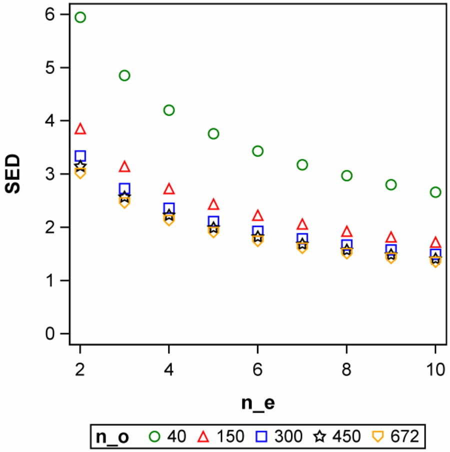
Fig. 2. Colour online. Plot of SED versus ne for no = 40, 150, 300, 450, 672. Trait: Stem weight.

Fig. 3. Colour online. Plot of SED versus ne for no = 2, 5, 10, 20, 59. Trait: Plant height.

Fig. 4. Colour online. Plot of SED versus ne for no = 2, 5, 15, 50, 72. Trait: Culm number.
The analyses so far have provided some insights, but have not settled the question of optimal sample size. We may consider two specific questions: (i) Was the chosen sample size no sufficient for the current trial, where ne = 4? (ii) What are the best numbers of plots (ne) and samples per plot (no) for a future trial? These are two different questions, and the answer in each case depends on the precision requirement. We will consider both questions in turn, using one trait at a time. For stem circumference, the smallest difference considered relevant is taken to be δ = 1 mm. For no = 40 as used in the current trial, the variance of a plot mean equals:

To detect a difference of δ = 1 mm at α = 5% with a power of 80%, we need:

plots per treatment (Eqn 31), which is the number of plots in the current trial. Conversely, using Eqn (53), we find that for a given number of ne = 4 plots:

samples would be needed, which is less than the number in the current trial, so there is scope for reducing sample size a bit for this trait.
Turning to the second question, we use the optimal allocation no = 212, for which:

Here, we would only need:

plots per treatment. If in consideration of other traits, however, we decide to stick with ne = 4 plots, we would need to use the sample size no = 29 found above.
Next, consider the trait stem weight. The individual specific stem weights were measured here so the two variance components for plots and samples could be estimated. Otherwise, for statistical analysis comparing treatments, we only need the plot means. This suggests that the 10 cm stem sections harvested for a plot can be pooled and the bulk weight determined and divided by the number of stems, thus reducing co and facilitating an increase in no. The fact that the sample variance is very much larger than the plot variance suggests that a large number of samples per plot is indeed very advantageous, and the plot in Fig. 2 also bears this out, considering the marked drop in SED when increasing no from 40 to 150. If δ = 10 mg is considered as the smallest relevant difference, then ne = 6 plots per treatment are required to achieve a power of 80% at α = 5% when no = 40. By comparison, when no = 70 the required plot number is no = 4, and when no = 100, only ne = 3 plots are needed.
To conclude the example, we briefly consider the remaining two traits. For plant height, δ = 10 cm may be considered the smallest relevant difference. Applying Eqn (53) yields a negative value for no, indicating that the number of ne = 4 plots is not sufficient to detect such a difference. Hence, we determine the variance of a plot mean with the optimal allocation no = 59 as σ 2 = 68.85 and find the necessary number of plots per treatment from (31) as ne = 11 (α = 5%, power = 80%). This is much larger than the number of plots usually used, and we may not be prepared to increase the trial to this size. The calculations indicate, however, that with a smaller plot number we cannot expect sufficient precision for this trait. To improve precision (reduce $\sigma _o^2$ ), one could also consider estimating individual stem heights rather than that of a collection of plants on a 50 × 50 cm2 sub-plot. Measuring the height of 30 or 40 individual stems per plot seems feasible. For culm number, we may use δ = 10 as the smallest relevant difference (α = 5%, power = 80%). As before, Eqn (53) shows that ne = 4 plots is not a sufficient number of replications. Applying the optimal allocation yields σ 2 = 126.76, and using this in (31) yields ne = 20 plots, which is clearly beyond feasible limits, indicating that it will not be possible to detect relevant treatment differences for this trait. Again, it may be worth devising an improved method for assessing this trait at the plot level.
Series of trials
Several sites
Series of trials have a long history, and in agriculture, perhaps the most prominent use case is variety of trials (Yates and Cochran, Reference Yates and Cochran1938). Consider a set of variety trials conducted at several sites and each laid out in randomized complete blocks. The purpose is to assess the mean performance of the tested varieties in a target population of environments (Atlin et al., Reference Atlin, Baker, McRae and Lu2000), and the sites used to conduct the trials are thought to be representative of this population. Hence, sites are modelled as a random factor and the following LMM is used for analysis:

where μ is an intercept, g i is the main effect of the ith genotype, s j is the main effect of the jth site, (gs)ij is the interaction of the ith genotype and the jth site, b jk is the effect of the kth replicate at the jth site, and e ijk is the plot error. Assuming that the data is entirely balanced and all effects indexed by sites are random with constant variance, the variance of a difference (VD) of two genotype means (μ + g i) is given by (Talbot, Reference Talbot1984):

where $\sigma _{gs}^2$ is the genotype-by-site (genotype-by-environment) interaction variance, $\sigma _e^2$
 is the plot error variance, n s is the number of sites and n r is the number of replicates per site. The SED is then given by $SED = \sqrt {VD}$
 . Notice the similarity of the expression in brackets in Eqn (55) with the variance given in Eqn (50), which is no coincidence. In fact, we can exploit this analogy to find the optimal number of replications per site, provided that variable costs can be obtained for each additional plot (c r) and for each additional trial site (c s). Then the optimal number of replications per site is given by (Snedecor and Cochran, Reference Snedecor and Cochran1989, p. 448):

Either with this number of replications per site, or the number of replications determined by other considerations, the required number of sites n s can be determined using the methods for two means in the third section, setting n s = n and:

If cost plays no crucial role, returning to Eqn (55), it may be observed that for a given total number of plots, nrns, VD would be maximized by setting nr = 1 and thus maximizing the number of sites, ns. It must be borne in mind, however, that with one replication only it is impossible to assess the precision of an individual trial or identify outliers based on an analysis of residuals.
We also note the close links of VD in Eqn (55) with broad-sense heritability, which is often used by breeders to assess the efficiency of their trialling system (Atlin et al., Reference Atlin, Baker, McRae and Lu2000). Assuming that genotypic main effects g i have variance $\sigma _g^2$ , this is given by (Piepho and Möhring, Reference Piepho and Möhring2007):

This equation may appear a bit unusual but is, in fact, easily seen to be equivalent to the common equation for broad-sense heritability (Nyquist, Reference Nyquist1991):

The main advantage of (58) is that it is amenable to straightforward generalization to all kinds of departures from the simple assumptions made here, including heterogeneity of variance, incomplete block designs, unbalanced data, or spatial analysis (Piepho and Möhring, Reference Piepho and Möhring2007). We are making this link with heritability here to point out that maximizing H 2 for given $\sigma _g^2$ is much the same thing as minimizing VD or SED. The simple Eqn (59) can be used with pre-determined value of sn r to yield a portable expression for n s as a function of the desired value of H 2:

where σ 2 is as given in (57). This kind of equation was considered by Yan (Reference Yan2021), who further suggested to generally require H 2 = 0.75, in which case (60) simplifies to $n_s = {{3\sigma _g^2 } / {\sigma ^2}}$ . As convenient as this may seem, we think this latter requirement for H 2 is taking the idea of portability one step too far, as the desirable and achievable level of H 2 is usually quite context-specific and, among other things, depends on the trait and the stage of the breeding programme.
Several sites crossed with years
A second important case occurs when the trials are also replicated across years at the same sites. In this case, again assuming balanced data, the VD in (52) extends to (Talbot, Reference Talbot1984; Casler, Reference Casler2015):

where $\sigma _{gy}^2$ is the genotype-by-year interaction variance, $\sigma _{gsy}^2$
 is the genotype-by-site-by-year interaction variance, and n y is the number of years. The optimal allocation problem now involves three variables, n r, n s and n y, which is a bit more complex at first sight. In practice, however, the number of years, n y, is usually fixed, or only has very few options, so we can regard this as a given in most applications. In this case, the term in (61) involving $\sigma _{gy}^2$
 is a constant and does not affect the optimization problem. In fact, it is sufficient to consider the same optimization as in Eqn (56) using $\tilde{\sigma }_{gs}^2 = \sigma _{gs}^2 + n_y^{{-}1} \sigma _{gsy}^2$
 and $\tilde{\sigma }_e^2 = n_y^{{-}1} \sigma _e^2$
 in place of $\sigma _{gs}^2$
 and $\sigma _e^2$
 , respectively.
It is also worth stressing that ny is typically smaller than ns, resulting from the fact that it is more difficult to add more years than to add more sites. For the same reason, there is sometimes a suggestion to replace years by sites. Such suggestions are unhelpful, however, when the genotype-year variance is non-negligible. This is because the only way to reduce its effect on VD is to increase ny as is apparent from Eqn (61).
Example 16: Post-registration variety trials conducted in the German federal state of Mecklenburg-Vorpommern typically comprise 25–30 varieties and fall into two broad categories, depending on the crop: (i) single-factor experiments with variety (genotype) as the only treatment factor, and (ii) two-factor experiments with management intensity as a second factor. Trials in category (i) usually have four replications, sometimes three, whereas trials in category (ii) typically have two replications, sometimes three. We here consider the design for a single-factor scenario. Variance components for yield (× 10−1 t/ha) were obtained from regional wheat variety trials (Table 16). The trials were two-factorial but these were analysed by intensity level, amounting to a single-factor analysis as appropriate for our purpose here. These analyses are based on a two-stage approach, in which variety means and associated standard errors (SEM) are computed in the first stage and then are submitted to a weighted mixed model analysis in which the inverse of the squared standard errors are used as weights (Piepho and Michel, Reference Piepho and Michel2000). This approach accounts for the heterogeneity of error variances between trials. Here, for the purpose of planning trials, we are assuming a constant variance as an approximation and that designs will be laid out in complete blocks.
Table 16. Variance component estimates (obtained by residual maximum likelihood) for yield ( × 10−2 t2/ha2) in post-registration wheat variety trials in Mecklenburg-Vorpommern (Landesforschungsanstalt für Landwirtschaft und Fischerei)

a To obtain an estimate of the error variance $\sigma _e^2$ , we computed the average SEM, squared this and multiplied by 2.5, the average number of replications across all trials.
Using the variance components in Table 16, Fig. 5 shows plots of SED for different values of ny (1, 2, 3, 4, 5), ns (1, 3, 5, 7, 9), and nr (1, 2, 3, 4). The choice nr = 2 is a frequently used number of replications used in a series of variety trials, whereas nr = 4 is less common. The figures show two horizontal reference lines, one at SED = 4 (× 10−1 t/ha) and one at SED = 2 (× 10−1 t/ha). These two lines are based on the researchers’ assessment and delineate the range of precision they require, first to make tentative recommendations and then making final recommendations at a later stage. The results show that the most crucial factor is the number of years ny. With only one year of testing, at least nine sites are required to achieve SED = 4, the number of replications having relatively little impact. By comparison, with two years of testing, about the same precision of SED = 4, considered appropriate for preliminary recommendations, can already be achieved with three or four sites. Sufficient precision for final recommendations at SED = 2 is only achieved after four to five years with more than five sites.

Fig. 5. Colour online. Standard error of a difference (SED; in 10−1 t/ha) as per (61) with $SED = \sqrt {VD}$ for variance components $\sigma _{gs}^2$
 , $\sigma _{gy}^2$
 , $\sigma _{gsy}^2$
 , and $\sigma _e^2$
 as shown in Table 16 for different values of ny (1, 2, 3, 4, 5) = number of years, ns (1, 3, 5, 7, 9) = number of sites, and nr (1, 2, 3, 4) = number of replicates. Reference lines on ordinate at SED = 4 (× 10−1 t/ha) (desirable for early assessment) and SED = 2 (× 10−1 t/ha) (desirable for recommendations).
We have assumed here that the error variance is constant and does not change with the number of replications. In this regard, it is worth adding that the current practice in the post-registration trials conducted by the federal state is to use row-column designs, where complete blocks can be formed by groups of rows or columns, or by single rows or columns (Piepho et al., Reference Piepho, Williams and Michel2021). A standard analysis according to a randomized complete block design can always be used if the additional row or column blocking proves ineffective. A model selection routine has been implemented that checks this via information criteria. In addition, spatial covariance structures are fitted, and this add-on, as well as the incomplete column blocks often improve precision. This is particularly true of larger trials showing marked irregular spatial heterogeneity throughout the field, and the chances of an improved fit with such more complex models increase with the number of replications. Even though this has not yet been comprehensively evaluated, in practice, there is a tendency for the SED of individual trials to drop with increased nr at a somewhat higher rate than expected from the simple Eqn (23). Thus, our usage of the simple Eqn (61) constitutes an approximation. We also stress the importance of having nr > 1 so that individual trials can be analysed in their own right, including critical scrutiny of outliers, and trials can be weighted by their precision in an analysis across environments (Piepho and Michel, Reference Piepho and Michel2000).
Several sites nested within years
A third case occurs when the sites change completely each year, meaning that sites are nested within years. In this case, the two-way interaction variance $\sigma _{gs}^2$ is confounded with $\sigma _{gsy}^2$
 and so cannot be separately estimated. The VD becomes:

where ns is the number of sites used in each year, so the total number of sites used in ny years is nsny. The most important point here is that this VD will always be smaller than or equal to that in (61) for the same values of n r, n s and n y and the same values of the variance components, showing that a change of sites each year is generally desirable in terms of efficiency. The advantage is most pronounced when $\sigma _{gs}^2$ is large relative to the other variance components. Again, the term in (62) involving $\sigma _{gy}^2$
 is a constant and it is sufficient to consider the same optimization as before this time using $\tilde{\sigma }_{gs}^2 = n_y^{{-}1} ( {\sigma_{gs}^2 + \sigma_{gsy}^2 } )$
 and $\tilde{\sigma }_e^2 = n_y^{{-}1} \sigma _e^2$
 in place of $\sigma _{gs}^2$
 and $\sigma _e^2$
 , respectively.
Example 16 (cont'd): Using the variance components in Table 16 with nr = 2, ns = 7, and ny = 5, we find SED = 2.03 (× 10−1 t/ha) for the crossed design (Eqn 61) and SED = 1.89 (× 10−1 t/ha) for the nested design, demonstrating the advantage of the latter. Whereas Eqns (61) and (62) represent the two competing design options of sites crossed with, or nested within years in pure form, in practice there is often a mix between both, with some sites used in more than one year and others used only in single years within a series of trials. This is especially true when transitioning from a design where all sites are used in all years, to a trialling system with new sites being added each year and the number of sites increasing towards later years, as is the current practice with post-registration trials in Mecklenburg-Vorpommern. Explicit equations evaluating the design efficiency are more complex (Laidig and Utz, Reference Laidig and Utz1992), and a computer-based approach as discussed in the next section is more convenient.
Using a linear model package to compute precision and power
All examples considered so far were tackled by easy-to-compute (portable) equations. In this section, we briefly review generalizations of the methods considered so far that allow determining sample size, precision and power for any design based on a LM even when simple explicit equations are not available, e.g. when using designs with incomplete blocks rather than complete blocks. As this more general approach is not usually amenable to manual computation, it is certainly not as portable as the approaches reviewed so far and so will not be considered in detail here. However, the underlying principles are the same, and with a good computer and statistical package computation is straightforward. Detailed illustrations will be found in the cited references and in a companion paper, which is under preparation.
Numerical approximations
In all cases considered so far, simple explicit equations were available for the SED as a function of n, which was the basis for obtaining explicit equations for the necessary sample size. Quite often, however, the model or the structure of the design may mean that such convenient expressions for sample size are not available. In these cases, one can always resort to the matrix formulation of the LM at hand and corresponding matrix expressions for SED. We will not consider these matrix expressions here and refer the interested readers to pertinent textbooks and papers (McLean et al., Reference McLean, Sanders and Stroup1991; Searle et al., Reference Searle, Casella and McCulloch1992). Suffice it to say that for LM, having the residual error term as the only random effect, exact calculations are always possible, whereas with LMM some kind of approximation is usually needed (Kenward and Roger, Reference Kenward and Roger1997). We skip these details because the computation can be left to a good mixed model package that has a facility to fix variance components at pre-specified values. The main task for the researcher then is to set up a dataset for the contemplated design and fit the model corresponding to the design at hand to a dummy response variable. The structure of the dataset must be the exact same as would be used for analysis of data obtained in the planned experiment. Then for pre-specified variance component values the package will compute the SED for the comparisons or contrasts of interest (Stroup, Reference Stroup2002; Casler, Reference Casler2015). The main point to appreciate here is that the SED really only depends on the design and the variance components, but not on the actual data. Thus, we can set the dummy response in our dataset to any numerical value. This is what makes the approach feasible at the design stage. In the special cases considered in the preceding sections, this package-based approach will return exactly the same SED as the explicit equations given in this paper. So we are still doing the same thing as before but just with some more flexibility as regards the model, the structure of the data and the design.
The only slight inconvenience of this whole approach is that it does not give us the optimal sample size in one go. Instead, it returns the SED for a given design, which among other choices entails a specific choice of sample size. So what we need to do is try designs of increasing size until we find one with approximately the desired SED.
We may also consider planning sample size with a significance test in mind. Here, we need to compute the power, 1 − β, for designs with increasing sample size until we achieve the desired power (Stroup, Reference Stroup2002). As before, we will focus on the comparison of two means (μ 1 and μ 2), which will always be done by a t-test. Hence, the exact power calculation involves the central and non-central t-distributions of the test statistic under the null and alternative hypotheses, whereas the approximate calculation uses the standard normal distribution to approximate both distributions. Here, we will first consider the normal approximation and then look at the exact solution. The test statistic is:

where $\hat{\mu }_1$ and $\hat{\mu }_2$
 are the two mean estimates under the fitted LMM. Equation (63) assumes that the SED is known, in which case t has a normal distribution. When SED is replaced by an estimate, this turns into a t-distribution. Note that this reduces to (30) for the simple t-test, which involves arithmetic means of the data in each group, whereas the model-based mean estimates here can take different forms and do not usually have such simple algebraic expressions. Again, we can rely entirely on the package to do the computations for us.
Under the null hypothesis H 0, t in (63) has an approximate standard normal distribution with unit variance and mean zero. Hence, we will reject the null hypothesis when |t| > z 1−α/2 as usual. Under the alternative hypothesis HA, when the difference between the means equals δ = μ 1 − μ 2, t has an approximate normal distribution with unit variance and mean δ/SED. All we need to do then is work out the probability under HA that |t| > z 1−α/2, i.e. either t < −z 1−α/2 or t > z 1−α/2. This probability is the power 1 − β for the given design. For this calculation, we just need a function for the cumulative distribution function of the standard normal, denoted as Φ(.). Then the two required rejection probabilities are:

Adding up, the power is:

This approximate calculation is entirely general and works for any LMM. All we need to do is get the SED from our package as described above and plug it into (64). The more exact calculation replaces z 1−α/2 with t 1−α/2, the critical value of a central t-distribution with appropriate residual degrees of freedom (Welham et al., Reference Welham, Gezan, Clark and Mead2015, p. 248). Likewise, the normal distribution under HA is replaced by the noncentral t-distribution with appropriate degrees of freedom and noncentrality parameter δ/SED. The appropriate degrees of freedom will be the residual degrees of freedom for LM, in which case the power calculation is indeed exact, whereas for LMM the degrees of freedom often have to be approximated (Kenward and Roger, Reference Kenward and Roger1997), meaning that the whole power calculation will still be approximate. A more accurate power calculation, properly dealing also with the degrees-of-freedom issue, can be conveniently obtained by simulation, and this will be discussed in the next sub-section. Here, we restrict attention to the normal approximation, which is in line with all the portable equations given so far, and which will be sufficient for most practical purposes, unless the residual degrees of freedom are very small.
The general approach just described may also be turned into a generalization of the simple rule given in Eqn (38), where we pre-specify the desired power. Even the simple 1-2-3 rule of thumb can still be applied, i.e. make sure SED is no greater than |δ|/3 when desiring a power of 85% at α = 5%. Similarly, if the focus is on the estimation of effect size, make sure the SED is no greater than $\tau _\delta /2$ or EHW/2 (Eqn 37). These rules are portable indeed, as they work for any LMM. Also, they obviate the need to explicitly calculate the power but only require evaluating the SED for candidate designs.
Simulating power and precision
The analytical approach described in the previous sub-section often works fine for LMM when only the SED is required. By contrast, EHW and power calculations require appropriate denominator degrees of freedom, and these may need to be approximated depending on the design and model (Kenward and Roger, Reference Kenward and Roger1997). Generally, in small samples, the plug-in approach of the previous sub-section may not be sufficiently accurate. In such settings, a simulation approach may be preferred (Gbur et al., Reference Gbur, Stroup, McCarter, Durham, Young, Christman, West and Kramer2012; Green and MacLeod, Reference Green and MacLeod2015). Also, generalized LMMs involve an extra layer of approximation because the likelihood needs to be approximated, and all inference (significance tests, confidence intervals) is only approximate as well (Wolfinger and O'Connell, Reference Wolfinger and O'Connell1993; Bolker et al., Reference Bolker, Brooks, Clark, Geange, Poulsen, Henry, Stevens and White2009; Stroup, Reference Stroup2013). Thus, simulation is often the method of choice. An important added benefit of simulation is that it allows assessing the validity of nominal Type I error rates for significance tests and confidence intervals, which may be worth checking in their own right, especially when one or several random effects are associated with only limited degrees of freedom.
The simulation approach works similar to the analytical approach in that a data frame with the same structure as the contemplated design is generated. Next, a large number of datasets with this structure are simulated according to the same model that will be used for analysing the data. The intended analysis is then applied to all simulated datasets and measures of precision (SED, EHW) and power (significance) are computed. These measures (means, quantiles, etc.) may then be summarized across all simulated datasets. For assessing the SED, we may compute the root mean squared deviation of the estimated and true difference. Thus, in each simulation run (i.e. for each simulated dataset), we compute $( {\delta -\hat{\delta }} ) ^2$ and then these squared deviations are averaged across simulation runs. In general, the mean squared deviation would also comprise bias, but from the properties of generalized least squares estimation, we may assume that the estimators are unbiased for LMM (Kackar and Harville, Reference Kackar and Harville1981). Thus, the root mean squared deviation assesses the SED. This estimate of SED can be compared to the model-based estimates of SED. Moreover, for each simulation run, we may obtain the HW of a confidence interval and average this over the simulation runs. Power may be assessed by simply computing the proportion of simulation runs in which the simulated test rejected the null hypothesis at the nominal significance level α. Since simulations are based on independent datasets, a confidence interval for the power of the test can be computed based on a binomial distribution.
Discussion
Sample size, or the number of replications, concerns only one of the three basic principles of experimental design, otherwise known as Fisher's 3 R's (Preece, Reference Preece1990), i.e., replication, randomization and (‘r’) blocking (local control). Thus, having determined a suitable sample size does not settle all design issues. In fact, good blocking may reduce the error variance σ 2, thus allowing a smaller sample size to be used than under complete randomization. When the design involves incomplete blocks, specialized methods can be used to generate good designs for an increasing series of replication numbers (e.g. Edmondson, Reference Edmondson2020; Piepho et al., Reference Piepho, Williams and Michel2021) and then the methods in the previous section can be used to evaluate the precision and power.
Depending on the textbook one picks up on sample size, one may end up with different formulae. This can be confusing both to the consulting statistician and the research scientist. One potential source of confusion is that equations are often presented in isolation from alternative approaches. This tutorial has provided an overview of different approaches and elucidated the close interconnections between them. The key quantity that connects all procedures is the standard error of an effect size estimate. Most of the time, the effect size of interest will be a difference of means, possible on a transformed scale, in which case the focus is on the SED. The portable procedures we have reviewed provide approximate estimates of sample size, and we believe that this is usually sufficient. Our review does not claim any degree of completeness. While we have covered basic procedures for one or two means quite comprehensively, our treatment of other scenarios was necessarily selective and reflects our own backgrounds. The general procedures reviewed in the previous section can help practitioners to think effectively and decide about sample size in their own research or in the statistical consulting they provide, even if the problem at hand initially does not seem straightforward or covered by any canned solutions. A detailed exemplification of these computer-based approaches will be provided in a companion paper.
In the previous section, we also focused on the SED and pairwise comparisons, as in the sections before. The proposal of Stroup (Reference Stroup2002) is focused on significance testing using the F-test. This is equivalent to a t-test when the F-statistic has a single degree of freedom for the linear hypothesis being tested, as is the case with a pairwise comparison. In keeping with our focus on pairwise comparisons throughout this paper, we have fully relied on that equivalence. The examples also showed that the same approach can easily be used to assess SED, and that applying the 1-2-3 rule to the SED of contending designs provides a convenient and simple approach to designing a trial.
Our treatment of significance tests has assumed that the test will be two-sided, i.e., there is a point null hypothesis such as H0: δ = 0 and the alternative covers both sides of H0, i.e. δ > 0 and δ < 0. It is emphasized here, however, that in some applications it may be more appropriate to consider one-sided null hypotheses of the form H0: δ ⩽ 0, with corresponding alternative hypothesis HA: δ > 0. For example, in experiments with animals, it may only be of interest to demonstrate that a new treatment is superior to a control. In the same vein, one may also construct one-sided instead of two-sided confidence intervals. The practical consequence of a one-sided significance test or confidence interval is that for the same level α the required sample size is lower than for the corresponding two-sided procedure. This has prompted some ethics committees and other official bodies deciding on the approval of experiments with animals to make the one-sided procedure the default assumption, requiring the experimenter to provide convincing arguments in case a two-sided procedure is proposed. Our view is that in most applications both sides of departure from a point null hypothesis are relevant, even though the consequences may depend on the side. This is why we have only considered two-sided tests or intervals. If one decides that the procedure needs to be one-sided, then the 1 − α/2 quantile of the standard normal distribution can be replaced by the 1 − α quantile in the relevant equations given in this paper, with an associated drop in the necessary sample size. For details see, e.g., Rasch et al. (Reference Rasch, Pilz, Gebhardt and Verdooren2011).
Conclusion
Here is our portable take-home message in case estimated treatment means are approximately normal, the 1-2-3 rule: Design your sample size in terms of a suitable requirement for the value of the standard error of the effect you are targeting. This will usually be a SED because most experiments are comparative. According to the 1-2-3 rule, there are three options for setting the SED:
(1) You can define the required precision directly in terms of a targeted value of SED itself.
(2) If you target a specific allowable deviation τδ of an estimator or EHW of a confidence interval, set SED = τδ/2 or SED = EHW/2. Conversely, based on a given value for the SED, it may be stated that at α = 5% the EHW of a 95% confidence interval is 2 × SED.
(3) If you are considering a significance test with the smallest relevant effect size δ, set SED = δ/3. Conversely, based on a given value for the SED, it may be stated that the smallest relevant difference that can be detected with a power of 85% is 3 × SED.
Acknowledgements
We thank Mario F. D'Antuono (Perth, Australia) for very helpful comments on an earlier draft of this paper. Thanks are also due to Georg Petschenka (University of Hohenheim, Stuttgart, Germany) for his help in putting together Example 10, and to Hans-Georg Schön (Hochschule Osnabrück, Germany) for his help with Example 4.
Author contributions
HPP conceived and designed the study. DG and JH implemented and checked all calculations using statistical packages and helped editing the paper. AB, MG, SK, FL, VM, IP, JES, KT and DW helped developing the examples and editing the text for these.
Financial support
This research received no specific grant from any funding agency, commercial or not-for-profit sectors.
Conflicts of interest
The authors declare there are no conflicts of interest.
Ethical standards
Not applicable. Where data on vertebrates was used, this was published data.
Appendix
Example 11: We need to point out that on the surface we have determined sample size here based on the binary distribution for the transformed response of the individual animals, using σ 2 = 1/4. This is the limiting case of a binomial distribution with m = 1. However, the approximate variance for the angular-transformed binomial in (40), which is based on a Taylor-series expansion, requires m ≫ 1 (McCullagh and Nelder, Reference McCullagh and Nelder1989, p. 137). To justify our approach, consider the following argument (also see Paulson and Wallis, Reference Paulson, Wallis, Eisenhart, Hastay and Wallis1947; cited in Cochran and Cox, Reference Cochran and Cox1957, p. 27). The count of level A in a group may be regarded as a single binomial count c for sample size m. In this view, n = 1 for both groups, and our task is to find the optimal binomial sample size m. So we may set n = 1 and σ 2 = 1/(4m) in (31) with δ as given in (42). Solving this for m yields

justifying our use of Eqn (31) even for a binary variable.


 Open access