

1. Introduction
Coherent structures in wall-bounded turbulence play a crucial role in turbulence research due to their significant turbulent momentum and heat transport. Consequently, they have been a focus of numerous experimental, theoretical and numerical studies spanning several decades (the reader is referred to Robinson (Reference Robinson1991), Adrian (Reference Adrian2007), Smits, McKeon & Marusic (Reference Smits, McKeon and Marusic2011), Marusic & Adrian (Reference Marusic and Adrian2012) and Jiménez (Reference Jiménez2018) for reviews on the subject of coherent structures in wall-bounded turbulence).
Steadily, through the years, with the help of experiments and direct numerical simulations (DNSs), there has been ever-growing evidence of superstructures, large-scale motions and very-large-scale motions in turbulent channel, pipe and boundary layer flows (e.g. Kim & Adrian Reference Kim and Adrian1999; Marusic Reference Marusic2001; Ganapathisubramani et al. Reference Ganapathisubramani, Hutchins, Hambleton, Longmire and Marusic2005; Hutchins & Marusic Reference Hutchins and Marusic2007; Dennis & Nickels Reference Dennis and Nickels2011; Baltzer, Adrian & Wu Reference Baltzer, Adrian and Wu2013; Hwang et al. Reference Hwang, Lee, Sung and Zaki2016; Lee Reference Lee2017). The term superstructures is often associated with turbulent boundary layers, and these correspond to motions whose dimensions are significantly greater than the boundary layer thickness  $\delta _{TBL}$. In turbulent boundary layers, these motions were found to have streamwise wavelengths of the order of $6 \delta _{TBL}$ (Hutchins & Marusic Reference Hutchins and Marusic2007; Lee & Sung Reference Lee and Sung2011). Large-scale motions and very-large-scale motions, on the other hand, are usually associated with turbulent channel and pipe flows. In this context, large-scale motions have streamwise lengths greater than the outer length scale $h$ (half-channel width or pipe radius) but less than $3h$. Very-large-scale motions refer to motions whose streamwise length scales are greater than $3h$ (Lee et al. Reference Lee, Lee, Choi and Sung2014; Lee, Ahn & Sung Reference Lee, Ahn and Sung2015; Hwang et al. Reference Hwang, Lee, Sung and Zaki2016). Turbulent boundary layers, channel flows and pipe flows are termed canonical wall-bounded turbulence and superstructures, large-scale and very-large-scale motions are collectively termed large-scale motions (LSMs) from hereon. Despite significant quantitative differences, the LSMs are qualitatively similar across turbulent channel, pipe and boundary layer flows (Monty et al. Reference Monty, Stewart, Williams and Chong2007; Lee & Sung Reference Lee and Sung2013; Lee et al. Reference Lee, Ahn and Sung2015). The LSMs have been shown to carry significant portions of the turbulent kinetic energy (TKE) and Reynolds shear stress, with their energy content increasing with increasing Reynolds numbers. It should be noted that the LSMs do not directly correspond to the general integral-scale motions that are present in turbulent flows.
Compared with canonical wall-bounded turbulence, the turbulent structure of natural convection boundary layers (NCBLs) is poorly understood. The present study concerns a turbulent NCBL immersed in a stably stratified environment. However, as NCBLs immersed in stably stratified media share many qualitative similarities with their unstratified counterparts, the literature concerning the turbulent structure of unstratified NCBLs is briefly reviewed here.
Most early experiments and numerical simulations concerning turbulent NCBLs dealt with the mean streamwise velocity field, mean temperature field and one-point statistics (Gebhart Reference Gebhart1973). Using experiments, the mean streamwise velocity profiles, temperature profiles and heat transfer correlations at several Grashof numbers were reported by Eckert & Jackson (Reference Eckert and Jackson1950), Cheesewright (Reference Cheesewright1968) and Vliet & Liu (Reference Vliet and Liu1969). Vliet & Liu (Reference Vliet and Liu1969) also argued that the mean profiles of velocity and temperature fields in the outer layer could be approximated using universal power-law relationships.
There have been several attempts to understand the spatio-temporal structure of unstratified vertical NCBLs. Several numerical simulations and experiments were undertaken to uncover the flow structures in transitional unstratified NCBLs. It was shown that the NCBLs undergoing K-type and H-type transitions exhibit two-dimensional streamwise waves at the start of the transition. The  $\varLambda$-structures dominate the flow field during the later stages of transition, and these flow structures are qualitatively similar to the $\varLambda$-structures of transitional zero pressure gradient turbulent boundary layers despite differences in the flow dynamics (Zhao, Lei & Patterson Reference Zhao, Lei and Patterson2017, Reference Zhao, Lei and Patterson2019). For a Prandtl number Pr of 7.0, during the transition process, buoyancy contributes significantly towards TKE production when compared with the Reynolds shear stress (Zhao et al. Reference Zhao, Lei and Patterson2017). Experiments and numerical simulations also revealed that secondary mean flows in the form of longitudinal rolls also populate the NCBL during the transition process (Jaluria & Gebhart Reference Jaluria and Gebhart1974; Zhao, Lei & Patterson Reference Zhao, Lei and Patterson2016; Zhao et al. Reference Zhao, Lei and Patterson2017). A three-layer longitudinal system was observed during the K-type transition, while a two-layer longitudinal system was observed during the H-type transition (Zhao et al. Reference Zhao, Lei and Patterson2017).
Regarding turbulent NCBLs, Fujii (Reference Fujii1959), based on flow visualisation, argued the presence of a ‘vortex-street-like instability’ in the outer layer. Tsuji & Nagano (Reference Tsuji and Nagano1988a), apart from making detailed investigations into the mean profiles and one-point statistics, investigated the boundary layer structure close to the wall. The authors found that a viscous sublayer analogous to the linearly varying viscous sublayer in canonical wall-bounded turbulence is absent close to the wall. This was also confirmed in the high Grashof number DNS study of Ke et al. (Reference Ke, Williamson, Armfield, Norris and Komiya2020), where this behaviour was attributed to buoyancy effects. Tsuji & Nagano (Reference Tsuji and Nagano1988b) made accurate measurements of Reynolds shear stress and turbulent heat flux and confirmed the observations of Tsuji & Nagano (Reference Tsuji and Nagano1988a) regarding the unique turbulent structure of NCBLs. Nakao, Hattori & Suto (Reference Nakao, Hattori and Suto2017) investigated the turbulent structure of a spatially developing vertical NCBL using large-eddy simulation (LES) and showed that the outer layer was more turbulent than the inner layer at the Grashof numbers investigated. Using quadrant analysis (Wallace Reference Wallace2016) and flow visualisation, Hattori et al. (Reference Hattori, Tsuji, Nagano and Tanaka2006) and Nakao et al. (Reference Nakao, Hattori and Suto2017) showed that the turbulent structure was significantly different from what was observed in turbulent boundary layers. In this context, the inner layer is defined as the region between the wall and the maximum velocity location. The outer layer is the region between the maximum velocity location and the edge of the boundary layer (Tsuji & Nagano Reference Tsuji and Nagano1988b; Hattori et al. Reference Hattori, Tsuji, Nagano and Tanaka2006; Nakao et al. Reference Nakao, Hattori and Suto2017).
Experiments concerning turbulent vertical NCBLs by Lock & Trotter (Reference Lock and Trotter1968), Cheesewright & Doan (Reference Cheesewright and Doan1978), Kitamura et al. (Reference Kitamura, Koike, Fukuoka and Saito1985) and Hattori et al. (Reference Hattori, Tsuji, Nagano and Tanaka2006) revealed that the turbulent length scales are significant and that the large-scale eddies in NCBLs are essential for turbulent momentum and heat transport. The results from the DNS studies of Abramov, Smirnov & Goryachev (Reference Abramov, Smirnov and Goryachev2014) and Ke et al. (Reference Ke, Williamson, Armfield, Komiya and Norris2021) hinted at large-scale velocity structures in the outer layer of a temporally evolving unstratified NCBL. Large-scale structures were also observed in turbulent differentially heated channels (Versteegh & Nieuwstadt Reference Versteegh and Nieuwstadt1998; Ng et al. Reference Ng, Ooi, Lohse and Chung2017; Kim, Ahn & Choi Reference Kim, Ahn and Choi2021). Although large-scale eddies have been hinted at in several studies, there has yet to be a study that thoroughly investigates the statistical properties of these large-scale eddies.
The experiments of Tsuji, Nagano & Tagawa (Reference Tsuji, Nagano and Tagawa1992) revealed LSMs in the instantaneous temperature fields; however, the space–time correlations did not suggest the presence of streaks or bursts. This led the authors to conclude that the spanwise periodic streaky structures observed in turbulent boundary layers were absent in the temperature field of NCBLs. Abedin, Tsuji & Lee (Reference Abedin, Tsuji and Lee2012) also argued against well-ordered fluid motions in the velocity field of turbulent unstratified NCBLs.
Stable stratification is known to alter the mean flow and turbulent structure significantly. Ambient stable stratification is ubiquitous in many natural and industrial flows (Fan et al. Reference Fan, Zhao, Torres, Xu, Lei, Li and Carmeliet2021); yet, there is little research concerning NCBLs immersed in stably stratified media. Such flows arise in serval classes of natural ventilation problems where the ambient medium is often stably stratified (Bejan Reference Bejan2013). For example, such boundary layer flow could be observed along the interior surfaces of heated or cooled walls in buildings where the room is stably stratified. NCBLs immersed in stably stratified media are also often discussed in connection to differentially heated cavities (Gill Reference Gill1966; Gill & Davey Reference Gill and Davey1969). The differentially heated cavity and its corresponding boundary layer flow form a simplified representation of the fluid flow and heat transfer in fuel tanks, cooling of electrical equipment and solar collectors. Often such NCBLs are modelled using the one-dimensional formulation proposed by Prandtl (Reference Prandtl1952), referred to as the ‘buoyancy layer’ from hereon. In line with previous studies (Gill & Davey Reference Gill and Davey1969; McBain, Armfield & Desrayaud Reference McBain, Armfield and Desrayaud2007; Fedorovich & Shapiro Reference Fedorovich and Shapiro2009b; Maryada et al. Reference Maryada, Armfield, Dhopade and Norris2022), the current study uses the buoyancy layer to model an NCBL immersed in a stably stratified medium.
Like unstratified NCBLs, most studies on turbulent buoyancy layers focussed on the mean flow and one-point statistics (Fedorovich & Shapiro Reference Fedorovich and Shapiro2009a,Reference Fedorovich and Shapirob; Giometto et al. Reference Giometto, Katul, Fang and Parlange2017). Large-scale coherence of the streamwise velocity field was hinted by Schumann (Reference Schumann1990). Schumann (Reference Schumann1990) showed that large-scale coherence could exist in the outer layers of inclined and upright turbulent buoyancy layers using LES. For the vertical case, large-scale coherence of streamwise velocity was observed in the streamwise direction. For inclination angles where the heated surface was close to the horizontal, large-scale coherence was observed in the spanwise direction. However, limited conclusions can be drawn regarding the properties of LSMs resulting from such large-scale coherence due to the computational limitations of the study of Schumann (Reference Schumann1990).
1.1. Contributions of the present study
It is evident from the above literature that, despite being investigated for the better part of the last century, there is still no clear consensus on whether the LSMs are always present in NCBLs (both with and without stably stratified ambient media) and, if present, how they compare with LSMs in canonical wall-bounded turbulence. In an effort to clarify this long-standing issue, the existence of LSMs in a turbulent buoyancy layer is examined using DNS. An illustration of the problem at hand with the key findings is shown in figure 1.

Figure 1. An illustration of the problem at hand. (a) The high-speed (red contours represent the streamwise velocity perturbations  $u_2 = 2u_\tau$, with $u_\tau$ being the friction velocity as defined in § 2) and low-speed (blue contours represent the streamwise velocity perturbations $u_2 = -2 u_\tau$) LSMs in a turbulent buoyancy layer. The grey surface represents the heated wall with $\tilde {\vartheta } = 1$. (b) The non-dimensional temperature $\tilde {\vartheta }$ contours at $\tilde {\vartheta } = 0.7$ (red) and $\tilde {\vartheta } = -0.05$ (blue). Here, $x_1$, $x_2$ and $x_3$ are the wall-normal, streamwise and spanwise directions, respectively. The flow flows along the positive $x_2$ axis while the acceleration due to gravity $\boldsymbol {g}$ acts along the negative $x_2$ axis.
The buoyancy layer is defined in § 2 along with the computational details of the DNS.
The coherence, using two-point correlations, is investigated in § 3.2 where it is shown that the LSMs of streamwise velocity fluctuations are dominant in the outer layer of the buoyancy layer.
Unlike what is observed in unstratified NCBLs (Hattori et al. Reference Hattori, Tsuji, Nagano and Tanaka2006), the two-point correlations of streamwise velocity fluctuations exhibit signs of meandering, and this is examined in § 3.2.2. Here, it is demonstrated that the meandering is correlated with the sign of the spanwise velocity fluctuations.
The wall-normal coherence of LSMs is investigated in § 3.2.3. It is shown that the streamwise velocity fluctuations are coherent across significant wall-normal distances in the buoyancy layer, implying that large-scale eddies are dominant in vertical buoyancy layers.
The role of LSMs in TKE production is discussed in § 3.2.4. It is demonstrated that the LSMs, especially in the outer layer, are dynamically relevant and make considerable contributions towards the production of TKE.
Section 3.3 discusses the one-dimensional energy spectra of streamwise velocity fluctuations, where it is revealed that LSMs are the dominant energy-containing motions in the turbulent buoyancy layer.
2. Computational details
Let us consider a linearly heated vertical wall immersed in a stably stratified environment (positive vertical temperature gradient) such that the temperature difference ( $\Delta T$) between the heated wall (having temperature $T_w$) and the ambient medium (having temperature $T_\infty$) is a constant value ( $\Delta T = T_w - T_\infty = B$, where $B$ is an arbitrary constant). As the ambient medium has a positive vertical temperature gradient, the wall temperature must also increase similarly in the vertical direction to ensure $\Delta T=B$. This implies that $T_w$ and $T_\infty$ are functions of the vertical coordinate $x_2$. Here, following (Janssen & Armfield Reference Janssen and Armfield1996; McBain et al. Reference McBain, Armfield and Desrayaud2007; Zhao et al. Reference Zhao, Lei and Patterson2016, Reference Zhao, Lei and Patterson2017; Maryada et al. Reference Maryada, Armfield, Dhopade and Norris2022), we define $x_1$, $x_2$ and $x_3$ as the wall-normal, streamwise and spanwise directions, respectively. If $\Delta T = B$, an equilibrium NCBL with a constant boundary layer thickness develops on the heated surface, termed the buoyancy layer (Prandtl Reference Prandtl1952). The current study uses this to model an NCBL immersed in a stably stratified medium.
The flow is non-dimensionalised with the following velocity ( $U_{\Delta T}$) and length ( $\delta _l$) scales (Gill & Davey Reference Gill and Davey1969):
 \begin{gather} U_{\Delta T} = \Delta T \left( \frac{\boldsymbol{g} \beta \kappa}{\nu \gamma_s} \right)^{{1}/{2}}, \end{gather}
 \begin{gather}\delta_l = \left( \frac{4 \nu \kappa}{\boldsymbol{g} \beta \gamma_s} \right)^{{1}/{4}}, \end{gather}
where the thickness of the boundary layer is of the order of  $\delta _l$. Here, $\nu, \kappa, \boldsymbol {g}, \beta, \gamma _s$ are the kinematic viscosity, thermal diffusivity, acceleration due to gravity, coefficient of thermal expansion and the positive vertical temperature gradient, respectively. The magnitude of $\gamma _s$ defines the level/strength of stable stratification in the flow. As the ambient is stably stratified due to a positive vertical temperature gradient, let us assume $T_\infty = \gamma _s x_2$ and $T_w = B + \gamma _s x_2$ such that $\Delta T = B$ (Gill Reference Gill1966). Also, let us define $\tilde {\vartheta } = (T - T_\infty ) / \Delta T$, which is the temperature excess over the positive vertical temperature gradient scaled with $\Delta T$ (Gill & Davey Reference Gill and Davey1969; McBain et al. Reference McBain, Armfield and Desrayaud2007). The buoyancy frequency $N$ is $\sqrt {g \beta \gamma _s}$. Based on this non-dimensionalisation, the Reynolds number is defined as ${Re} = U_{\Delta T} \delta _l / \nu = (g \beta \Delta T \delta _{l}^3)/2\nu ^2$. It should be noted that the Reynolds number is half the Grashof number (
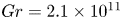
 $Gr = 2 {Re} = g \beta \Delta T \delta _{l}^3/\nu ^2$) in the current non-dimensionalisation (Gill & Davey Reference Gill and Davey1969).
With the above non-dimensionalisation, the following non-dimensional Navier–Stokes equation with the Oberbeck–Boussinesq approximation for buoyancy and the scalar transport equation are used to solve for the buoyancy layer (Gill & Davey Reference Gill and Davey1969; McBain et al. Reference McBain, Armfield and Desrayaud2007; Maryada et al. Reference Maryada, Armfield, Dhopade and Norris2022)
 \begin{gather} \frac{\partial \tilde{u}_i}{\partial x_i} = 0, \end{gather}
 \begin{gather}\frac{\partial \tilde{u}_i}{\partial t} + \tilde{u}_j \frac{\partial \tilde{u}_i}{\partial x_j} ={-} \frac{\partial \tilde{p}}{\partial x_i} + \frac{1}{{Re}} \frac{\partial^2 \tilde{u}_i}{\partial x^2_j} + \frac{2}{{Re}} \tilde{\vartheta} \delta_{i2}, \end{gather}
 \begin{gather}\frac{\partial \tilde{\vartheta}}{\partial t} + \tilde{u}_j \frac{\partial \tilde{\vartheta}}{\partial x_j} = \frac{1}{{Re}\,Pr} \frac{\partial^2 \tilde{\vartheta}}{\partial x^2_j} - \frac{2}{{Re}\,Pr} \tilde{u}_2, \end{gather}
where  $\tilde {\vartheta }$ is the instantaneous non-dimensional temperature, also called the buoyancy field (as defined in the previous paragraph), $\tilde {u}_i$ is the instantaneous non-dimensional velocity field, $\tilde {p}$ is the instantaneous pressure field, and $Pr = \nu / \kappa$ is the Prandtl number of the fluid. For the current non-dimensionalisation, the buoyancy time period ( $T_{SB} = {\rm \pi}{Re} \sqrt {Pr}$) (Gill & Davey Reference Gill and Davey1969; McBain et al. Reference McBain, Armfield and Desrayaud2007) is $2117.22$.
Figure 2 shows the coordinate system and a schematic of the NCBL in the relevant non-dimensional variables. It is evident from the figure that the stably stratified ambient medium causes the boundary layer to develop regions of flow reversal and  $\tilde {\vartheta }$ deficit, which are notably absent in unstratified NCBLs. The wall-normal distance between the linearly heated wall ( $\tilde {\vartheta } = 1$) and the location where the mean streamwise velocity changes sign for the first time (represented using a dashed vertical line in figure 2) is termed the boundary layer thickness $\delta _{bl}$. This definition is chosen as the mean flow does not asymptotically reach zero in the current flow, like unstratified NCBLs. Instead, due to the presence of a flow reversal, there is a well-defined location where the mean flow becomes zero and changes sign, allowing for a precise calculation of $\delta _{bl}$ based on the mean flow (this is also discussed in § 3.1).

Figure 2. The schematic representation of the vertical buoyancy layer showing the coordinate system and boundary conditions. Here,  $\tilde {u}_2$ is the streamwise velocity, and $\tilde {\vartheta }$ is the buoyancy field, the non-dimensional temperature field. The boundary layer thickness $\delta _{bl}$ is the wall-normal distance between the linearly heated wall and the blue dashed vertical line marked as BL. The inset shows the zoomed view of the flow reversal where $\tilde {u}_2$ is negative.
Throughout this paper, the instantaneous velocity and buoyancy fields are represented using  $\tilde {u}_i$ and $\tilde {\vartheta }$, respectively. Using Reynolds decomposition, the instantaneous fields are decomposed into the mean flow and fluctuating fields/perturbations. The mean flow fields are represented using $\bar {{\cdot }}$ and consequently, the mean streamwise velocity and buoyancy fields are indicated using $\bar {u_2}$ and $\bar {\vartheta }$, respectively. The fluctuating velocity and temperature fields are represented using $u_i$ and $\vartheta$ (such that $\tilde {u}_i = \bar {u_i} + u_i$ and $\tilde {\vartheta } = \bar {\vartheta } + \vartheta$). Averaged quantities of one-point turbulence statistics and correlations are represented using $\langle {\cdot } \rangle$. For the mean flow profiles and one-point turbulence statistics, the flow is averaged in time and the homogeneous streamwise ( $x_2$) and spanwise ( $x_3$) directions. The required quantities are averaged in time and the corresponding directions for the correlations.
A turbulent vertical buoyancy layer having a Prandtl number of 0.71 and a Reynolds number of 800 is investigated using DNS. It corresponds to a friction Reynolds number  ${Re}_\tau = u_\tau \delta _{bl} / \nu = 279.3$, where the boundary layer thickness is represented by $\delta _{bl}$, determined as the location where the mean streamwise velocity ( $\bar {u_2}$) changes sign for the first time (shown in figure 2). The friction velocity is represented using $u_\tau = \sqrt {\nu \partial \bar {u_2} / \partial x_1 |_w}$ (Ke et al. Reference Ke, Williamson, Armfield, Norris and Komiya2020). Here, the subscript $w$ indicates that the derivative is calculated at the wall.
Along with  ${Re}_\tau$, let us define $\delta ^{L_m} = \delta _{bl} / L_m$, which represents the ratio of the boundary layer thickness to $L_m = \nu ^{3/4} F_s^{-1/4}$. The buoyancy flux at the heated wall is represented using $F_s = - \alpha \partial \bar {\vartheta } / \partial x_1 |_w$ and $L_m$ is analogous to the Kolmogorov length scale (Fedorovich & Shapiro Reference Fedorovich and Shapiro2009a,Reference Fedorovich and Shapirob; Giometto et al. Reference Giometto, Katul, Fang and Parlange2017). This can be considered as the ratio of the length scale of the eddies that scale with $\delta _{bl}$ to the length scale of the eddies that scale with $L_m$, and provides an estimate on the range of scales present in the flow. In terms of $\delta ^{L_m}$ ( $\delta ^{L_m} \approx 400$ in the present case), the Reynolds number of 800 investigated in the current study is comparable to the range of parameters investigated in (Fedorovich & Shapiro Reference Fedorovich and Shapiro2009b; Giometto et al. Reference Giometto, Katul, Fang and Parlange2017). Developed turbulence was observed at these values of $\delta ^{L_m}$ (Fedorovich & Shapiro Reference Fedorovich and Shapiro2009b).
In the context of zero pressure gradient turbulent boundary layers, this  ${Re}_\tau$ can be considered low to moderate, and LSMs are seldom observed at such values of ${Re}_\tau$ (Hutchins & Marusic Reference Hutchins and Marusic2007; Smits et al. Reference Smits, McKeon and Marusic2011; Marusic & Adrian Reference Marusic and Adrian2012). However, that is not the case for the turbulent buoyancy layer. It is demonstrated in § 3 that this friction Reynolds number is sufficient to observe LSMs in the turbulent buoyancy layer. It should be noted that the LSMs are defined as motions whose streamwise length scales exceed the boundary layer thickness, in line with canonical wall-bounded turbulence literature (Lee et al. Reference Lee, Lee, Choi and Sung2014, Reference Lee, Ahn and Sung2015; Hwang et al. Reference Hwang, Lee, Sung and Zaki2016).
DNS was performed using an in-house non-staggered finite volume code (Norris Reference Norris2000; Armfield et al. Reference Armfield, Morgan, Norris and Street2003). The code has been used extensively to investigate natural convection flows, and its verification and validation are well documented (Armfield et al. Reference Armfield, Morgan, Norris and Street2003; Maryada et al. Reference Maryada, Armfield, Dhopade and Norris2022). The spatial terms were discretised using a second-order central difference scheme. Temporally, the advection and the diffusion terms were discretised using a second-order Adams–Bashforth scheme (Lilly Reference Lilly1965) and a second-order Crank–Nicolson scheme, respectively. A non-iterative fractional step method was used to solve for continuity (Armfield & Street Reference Armfield and Street2002). Collocated meshes are known to be susceptible to spurious oscillations in the pressure field, and Rhie–Chow interpolation (Rhie & Chow Reference Rhie and Chow1983) was used to avoid them. Rhie–Chow interpolation or related schemes retain the grid-scale ellipticity (Armfield Reference Armfield1994; Armfield et al. Reference Armfield, Morgan, Norris and Street2003), thereby avoiding the grid-scale oscillations in the pressure field. The velocity and scalar equations were solved using a generalised minimal residual (Saad & Schultz Reference Saad and Schultz1986) algorithm with a Jacobi preconditioner. The pressure Poisson equation was solved using the bi-conjugate gradient stabilised algorithm (van der Vorst Reference van der Vorst1992) with the strongly implicit procedure of Stone (Reference Stone1968) as a preconditioner. An appropriate time step was chosen such that the Courant number was always less than  $0.2$. Also, the divergence of the velocity field was checked after every time step and was always below $5 \times 10^{-10}$.
As the turbulent buoyancy layer is spatially homogeneous in the streamwise and spanwise directions, periodic boundary conditions were imposed in the streamwise and spanwise directions, in line with previous studies (Fedorovich & Shapiro Reference Fedorovich and Shapiro2009b; Giometto et al. Reference Giometto, Katul, Fang and Parlange2017; Maryada et al. Reference Maryada, Armfield, Dhopade and Norris2022). A no-slip boundary condition for velocity ( $\tilde {u}_i=0$) and a constant buoyancy ( $\tilde {\vartheta } = 1$) boundary condition were used at the heated wall. An open-type boundary condition where the flow can enter and exit the domain was used as the far-field boundary condition. At the open-type boundary, a zero gradient boundary condition normal to the boundary was applied for all the variables. In cases when flow enters the domain, it was set to have a constant temperature of $\tilde {\vartheta } = 0$, which corresponds to the flow as $x_1\to \infty$ (see figure 2). This boundary condition was also used while investigating transitional buoyancy layers (Maryada et al. Reference Maryada, Armfield, Dhopade and Norris2022).
The computational domain is  $2.18 {\rm \pi}\delta _{bl} \times 8 {\rm \pi}\delta _{bl} \times 3 {\rm \pi}\delta _{bl}$ in the wall-normal ( $x_1$), streamwise ( $x_2$) and spanwise directions ( $x_3$), respectively. In the wall-normal direction, the domain is bigger than the recommended wall-normal domain size of $3 \delta _{bl}$ often employed in DNS of boundary layer flows (Schlatter & Örlü Reference Schlatter and Örlü2010; Kozul, Chung & Monty Reference Kozul, Chung and Monty2016; Ke et al. Reference Ke, Williamson, Armfield, Komiya and Norris2021). Due to the large domain size, the boundary conditions at the far-field wall-normal domain boundary are not expected to affect the boundary layer flow. The domain size is similar to the domain size of Bae & Lee (Reference Bae and Lee2021) in the streamwise and spanwise directions and bigger than the domains previously used to investigate turbulent buoyancy layers (Schumann Reference Schumann1990; Giometto et al. Reference Giometto, Katul, Fang and Parlange2017). It should be noted that the domain size in the streamwise and spanwise directions is sufficient for the computed two-point correlations to decay to zero (evident from the results presented in § 3). This ensures that the numerical simulation results are not influenced by the periodic boundary conditions (Moin & Kim Reference Moin and Kim1982).
The domain has  $350 \times 1400 \times 550$ cells along the wall-normal ( $x_1$), streamwise ( $x_2$) and spanwise ( $x_3$) directions, respectively. Uniform grids were used in the streamwise and spanwise directions with $\Delta x_2^+ = \Delta x_3^+ = 4.95$, where $\Delta$ is the thickness of the cell. A semi-logarithmic mesh with a stretching factor of $1.01$ was used in the wall-normal direction with $\Delta x_1^+ = 0.42$ at the wall and $\Delta x_1^+ = 3.25$ at $x_1 = \delta _{bl}$. The distances represented with $^+$ are normalised by the viscous length scale ( $\delta _{\nu } = \nu / u_\tau = 0.042$). The mesh spacing employed is similar to the spacing commonly used in DNS of canonical wall-bounded turbulence and NCBLs (Hwang et al. Reference Hwang, Lee, Sung and Zaki2016; Ke et al. Reference Ke, Williamson, Armfield, Norris and Komiya2020; Bae & Lee Reference Bae and Lee2021; Ke et al. Reference Ke, Williamson, Armfield, Komiya and Norris2021). The Kolmogorov length scale $\eta = (\nu ^3 / \epsilon )^{1/4}$ was calculated a posteriori and it was found that $\Delta x_1 < \eta$, $\Delta x_2 < 3 \eta$ and $\Delta x_3 < 3 \eta$ everywhere inside the boundary layer. Here, $\epsilon = \nu \langle (\partial u_i / \partial x_j)(\partial u_i / \partial x_j) \rangle$ is the dissipation (Giometto et al. Reference Giometto, Katul, Fang and Parlange2017). It should be noted that $\eta$ is a function of the wall-normal distance (as $\epsilon$ is a function of the wall-normal distance), and the values of $\Delta x_i / \eta$ reported earlier represent the ‘worst case’ grid sizes. At the heated wall, $\eta = 0.074$ ( $\eta / L_m \approx 2.5$), and $\Delta x_1 < 0.25 \eta$, $\Delta x_2 < 3 \eta$ and $\Delta x_3 < 3 \eta$.
The DNS was run for nine buoyancy periods, and the statistics were calculated for the last four buoyancy periods. No significant differences were observed in the mean flow and turbulence statistics between the flow averaged for three and four buoyancy periods, indicating statistical convergence. It should be noted that the time period used to calculate statistics is in the range of values used by Giometto et al. (Reference Giometto, Katul, Fang and Parlange2017) for the turbulent buoyancy layer.
3. Results and discussion
3.1. Mean flow and turbulence statistics
Visualising the averaged mean flow and one-point statistics is worthwhile before investigating LSMs. The one-dimensional mean streamwise velocity and temperature profiles and their respective contour plots are shown in figure 3. In the figure, the boundary layer thickness,  $\delta _{bl}$, is defined as the wall-normal distance from the heated wall until the location where the mean streamwise velocity changes sign for the first time. It is clear from the figure that the mean streamwise velocity and buoyancy fields are qualitatively similar to the schematic shown in figure 2. The mean buoyancy field exhibits a region of temperature deficit while there is a distinct region of flow reversal in the mean streamwise velocity field (Schumann Reference Schumann1990; Fedorovich & Shapiro Reference Fedorovich and Shapiro2009a,Reference Fedorovich and Shapirob; Giometto et al. Reference Giometto, Katul, Fang and Parlange2017). The region of flow reversal extends in the range $1.0 \leq x_1 / \delta _{bl} \leq 2.0$ in figure 3(a,c). The region of temperature deficit is observed in the range $0.3 < x_1 / \delta _{bl} < 1.5$ in figure 3(b,d). The inner layer is classified as the wall-normal region between the heated wall and the wall-normal location where the mean streamwise velocity is maximum ( $0 < x_1 / \delta _{bl} \leq 0.065$). The outer layer is defined as the wall-normal region between the wall-normal location where the mean streamwise velocity is maximum and the flow reversal ( $0.065 < x_1 / \delta _{bl} \leq 1.0$). These plots demonstrate that the buoyancy layer is distinctly different from unstratified NCBLs where flow reversal and temperature deficit regions are not observed (Tsuji & Nagano Reference Tsuji and Nagano1988a; Abedin, Tsuji & Hattori Reference Abedin, Tsuji and Hattori2009; Ke et al. Reference Ke, Williamson, Armfield, Norris and Komiya2020, Reference Ke, Williamson, Armfield, Komiya and Norris2021).

Figure 3. Profiles of (a) mean streamwise velocity  $\bar {u_2}$ and (b) mean buoyancy $\bar {\vartheta }$ fields of the vertical buoyancy layer at ${Re} = 800$. The contours of $\bar {u_2}$ and $\bar {\vartheta }$ are shown in (c) and (d), respectively.
The variances of wall-normal, streamwise and spanwise velocity and buoyancy fluctuations are shown in figure 4(a). In the figure, the velocity variances are normalised using the square of the friction velocity ( $u_\tau ^2$) and the buoyancy variance is normalised using the square of the friction temperature ( $\theta _\tau ^2$). The definitions of $u_\tau$ and $\theta _\tau$ are consistent with Ke et al. (Reference Ke, Williamson, Armfield, Norris and Komiya2020, Reference Ke, Williamson, Armfield, Komiya and Norris2021). The mean streamwise velocity variance is greater than the wall-normal and spanwise velocity variance, suggesting that the streamwise velocity variance is the dominant contributor of TKE, as expected in turbulent boundary layer flows. Flow anisotropy is also evident from figure 4(a), hinting at the multiscale nature of the flow. The variance of all the velocity fluctuations exhibits a maximum in the outer layer at the Reynolds number investigated, implying that most of the turbulence associated with momentum transfer is present in the outer layer of the buoyancy layer. The peak in the streamwise velocity variance in the outer layer corresponds to a peak in the energy spectra of streamwise velocity fluctuations, which is discussed in § 3.3. In the inner layer, the variance of wall-normal velocity fluctuations decays faster than the variance of streamwise and spanwise velocity fluctuations and buoyancy fluctuations due to the presence of a wall.

Figure 4. One-point statistics of the turbulent vertical buoyancy layer at  ${Re} = 800$. (a) Mean velocity and buoyancy variances, and (b) mean Reynolds shear stress and wall-normal and streamwise turbulent heat fluxes. The dot-dashed black vertical line in both figures refers to the location of the velocity maximum, demarcating the inner layer from the outer layer. In (a), the vertical axis on the left corresponds to velocity variances, while the axis on the right corresponds to buoyancy variance. In (b), the vertical axis on the left corresponds to Reynolds shear stress, while the axis on the right corresponds to wall-normal and streamwise turbulent heat flux.
In contrast, the peak of the buoyancy variance is located in the inner layer close to the velocity maximum. This is the case as strong buoyancy gradients occur in this region (Fedorovich & Shapiro Reference Fedorovich and Shapiro2009b; Giometto et al. Reference Giometto, Katul, Fang and Parlange2017). In the wall-normal direction, the buoyancy variance decays faster than the velocity variances, implying that most buoyancy fluctuations are restricted to regions close to the heated wall, consistent with the observations of Giometto et al. (Reference Giometto, Katul, Fang and Parlange2017). This behaviour of velocity and buoyancy variances also agrees with what is observed in transitional buoyancy layers (Maryada et al. Reference Maryada, Armfield, Dhopade and Norris2022). Also, it is qualitatively similar to what is observed in turbulent differentially heated channels and unstratified NCBLs, where a peak in the streamwise velocity variance is observed in the outer layer (Tsuji & Nagano Reference Tsuji and Nagano1988b; Abedin et al. Reference Abedin, Tsuji and Hattori2009; Ng et al. Reference Ng, Ooi, Lohse and Chung2017). These plots highlight the stark differences between the present flow configuration and canonical wall-bounded turbulence. At comparable values of  $Re_\tau$, in canonical wall-bounded turbulence, there is a distinct peak in velocity variances close to the wall due to the inner wall cycle. An inner peak is absent in the present case, and turbulence is present mainly in the outer layer.
The wall-normal variation of Reynolds shear stress and the wall-normal and streamwise turbulent heat fluxes are shown in figure 4(b). Here, the Reynolds shear stress is normalised using  $u_\tau ^2$, and the turbulent heat fluxes are normalised using $\theta _\tau u_\tau$. The Reynolds shear stress is negative close to the wall in the inner layer and becomes positive with increasing wall-normal distance, in agreement with the observations of Fedorovich & Shapiro (Reference Fedorovich and Shapiro2009b) and Giometto et al. (Reference Giometto, Katul, Fang and Parlange2017). Similar behaviour is observed in unstratified NCBLs and turbulent differentially heated channels (Ke et al. Reference Ke, Williamson, Armfield, Norris and Komiya2020; Kim et al. Reference Kim, Ahn and Choi2021). A region of approximately constant Reynolds shear stress, commonly observed in turbulent boundary layers, is absent. On the other hand, the streamwise and wall-normal turbulent heat fluxes are always positive in the inner layer. These are also positive in the outer layer until $x_1 \approx 0.6 \delta _{bl}$. Both the wall-normal and streamwise turbulent heat fluxes are negative from approximately this wall-normal location and beyond, which agrees with the observations of Giometto et al. (Reference Giometto, Katul, Fang and Parlange2017). Also, the Reynolds shear stress peaks in the outer layer at $x_1 \approx 0.3 \delta _{bl}$ while the turbulent heat fluxes peak at locations much closer to the maximum velocity (still in the outer layer). The Reynolds shear stress and streamwise turbulent heat flux feature in the production of TKE. The production of TKE in relation to LSMs is discussed in § 3.2.4.
3.2. Two-point correlations
The existence of LSMs is investigated using two-point correlations (Ganapathisubramani et al. Reference Ganapathisubramani, Hutchins, Hambleton, Longmire and Marusic2005; Hutchins & Marusic Reference Hutchins and Marusic2007; Baltzer et al. Reference Baltzer, Adrian and Wu2013; Sillero, Jiménez & Moser Reference Sillero, Jiménez and Moser2014; Hwang et al. Reference Hwang, Lee, Sung and Zaki2016). The two-point correlation coefficient at a wall-normal plane of a fluctuating field  $\phi$, $R^T_{\phi \phi }$, is calculated using
 \begin{equation} R^T_{\phi \phi} = \frac{\langle \phi(x_2,x_3) \phi(x_2 + \Delta x_2,x_3 + \Delta x_3)\rangle}{\sigma_\phi^2}, \end{equation}
where  $\sigma _{\phi }$ is $\sqrt {\langle \phi ^2 \rangle }$. Throughout this paper, $\Delta x_2 > 0$ corresponds to the correlation downstream of the location of interest, and the correlation upstream of the location of interest corresponds to $\Delta x_2 < 0$.
The two-point correlation coefficients of  $\vartheta, u_1, u_2$ and $u_3$ in the streamwise direction at four different wall-normal locations are shown in figure 5. In the figure, the two-point correlation coefficient at $x_1 = 0.04 \delta _{bl}$ corresponds to a wall-normal location in the inner layer. The two-point correlations at the remaining wall-normal locations correspond to the outer layer. In the inner layer, the $u_1, u_3$ and $\vartheta$ fluctuations are positively correlated for $| \Delta x_2 | < 1$. The $u_2$ fluctuations, on the other hand, exhibit a positive correlation coefficient for $| \Delta x_2 | > 1$, hinting at the presence of LSMs. Qualitatively, the same conclusions also hold in the outer layer, with the width of the positive two-point correlation coefficient of $u_2$ being greater than the width of the positive two-point correlation coefficient of $u_1$, $u_3$ and $\vartheta$. The widths of the correlation of $u_1$ and $u_3$ become comparable with increasing wall-normal distance. The buoyancy fluctuations become increasingly correlated in the streamwise direction as one moves away from the wall. Figure 5 also strongly indicates that $u_1, u_2, u_3$ and $\vartheta$ fluctuations exhibit different length scales. As the widths of the two-point correlations of $u_1$, $u_3$, and $\vartheta$ are not comparable to the width of $R^T_{u_2 u_2}$, it can be presumed that the largest streamwise coherence is present for $u_2$. The width of $u_2$ fluctuations increases with increasing wall-normal distance, and these length scales of the $u_2$ fluctuations are discussed later using two-point streamwise–spanwise correlations.

Figure 5. The  $R^T_{u_2 u_2}$, $R^T_{\vartheta \vartheta }$, $R^T_{u_1 u_1}$, $R^T_{u_3 u_3}$ correlations in the streamwise direction at (a) $x_1 / \delta _{bl} = 0.04$,(b) $x_1 / \delta _{bl} = 0.1$, (c) $x_1 / \delta _{bl} = 0.3$ and (d) $x_1 / \delta _{bl} = 0.6$. The thick solid black curve represents $R^T_{u_2 u_2}$, thin red dashed curve represents $R^T_{\vartheta \vartheta }$, thick blue densely dash-dotted curve represents $R^T_{u_1 u_1}$ and thin green loosely dash-dotted curve represents $R^T_{u_3 u_3}$.
The two-point correlation coefficients of  $\vartheta$, $u_1$, $u_2$ and $u_3$ in the spanwise direction at four different wall-normal locations are shown in figure 6. In figure 6(a), close to the heated wall in the inner layer, the width of positive $R^T_{u_2 u_2}$ is greater than the width of positive $R^T_{\vartheta \vartheta }$, $R^T_{u_1 u_1}$ and $R^T_{u_3 u_3}$. However, the width of $R^T_{\vartheta \vartheta }$ becomes larger with increasing wall-normal distance, indicating that the spanwise coherence of buoyancy fluctuations becomes greater than the spanwise coherence of streamwise, wall-normal and spanwise velocity fluctuations. In the outer layer, the width of the positive correlation coefficient of $u_3$ and $\vartheta$ in the spanwise direction (figure 6) is comparable to the width of the positive correlation coefficient in the streamwise direction (figure 5), qualitatively similar to what is observed in unstratified NCBLs (Tsuji et al. Reference Tsuji, Nagano and Tagawa1992; Hattori et al. Reference Hattori, Tsuji, Nagano and Tanaka2006). Despite the spanwise coherence of $\vartheta$ and $u_3$ extending to greater distances than the spanwise coherence of $u_2$, it is still smaller than the streamwise coherence of $u_2$. This suggests that the $u_2$ fluctuations statistically exhibit the most prominent coherence. Therefore, the rest of the paper investigates the large-scale coherence of the streamwise velocity fluctuations, $u_2$.

Figure 6. The  $R^T_{u_2 u_2}$, $R^T_{\vartheta \vartheta }$, $R^T_{u_1 u_1}$, $R^T_{u_3 u_3}$ correlations in the spanwise direction at (a) $x_1 / \delta _{bl} = 0.04$, (b) $x_1 / \delta _{bl} = 0.1$, (c) $x_1 / \delta _{bl} = 0.3$ and (d) $x_1 / \delta _{bl} = 0.6$. The thick solid black curve represents $R^T_{u_2 u_2}$, thin red dashed curve represents $R^T_{\vartheta \vartheta }$, thick blue densely dash-dotted curve represents $R^T_{u_1 u_1}$ and thin green loosely dash-dotted curve represents $R^T_{u_3 u_3}$. Note that the horizontal scale differs from figure 5.
It should be noted that the two-point correlations of  $u_2$ in figure 6 become negative at $| \Delta x_2 | \gtrsim 0.5 \delta _{bl}$, which is absent in the two-point correlations of $u_2$ in the streamwise direction (see figure 5). Negative values of two-point correlations of $u_2$ in figure 6 suggest that alternating fast-moving and slow-moving structures are present in the flow. This is investigated in detail later in this section using streamwise–spanwise two-point correlations.
It should be stressed that the profiles of the two-point correlations of buoyancy fluctuations do not match the profiles of two-point correlations of the streamwise velocity fluctuations. It implies that relying on two-point correlations of the temperature field to investigate large-scale coherent motions in turbulent buoyancy layers would provide an incomplete picture of the boundary layer structure.
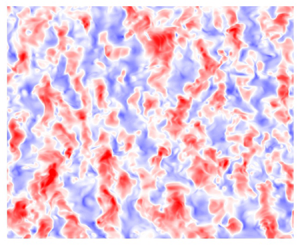
The long tails of two-point correlation coefficients merely suggest the presence of large-scale coherence. However, this does not provide insight into whether the large-scale coherence is due to LSMs or a chain of several small-scale structures (Sillero et al. Reference Sillero, Jiménez and Moser2014). Hence, examining the instantaneous flow structures helps us to understand the distribution of streamwise velocity perturbations. The instantaneous streamwise velocity perturbations at four different wall-normal locations are shown in figure 7. Streamwise-elongated streaky structures of high- and low-speed fluctuations dominate the figure. A high-speed velocity fluctuation refers to a positive streamwise velocity fluctuation, and a low-speed velocity fluctuation refers to a negative streamwise velocity fluctuation. The streamwise length of the  $u_2$ often exceeds the boundary layer thickness, consistent with the two-point correlations. This suggests that the large-scale coherence observed earlier in figure 5 is due to LSMs.

Figure 7. Instantaneous streamwise velocity fluctuations at (a)  $x_1 / \delta _{bl} = 0.04$, (b) $x_1 / \delta _{bl} = 0.1$, (c) $x_1 / \delta _{bl} = 0.3$ and (d) $x_1 / \delta _{bl} = 0.6$. Gravity acts in the negative $x_2$ direction, and the fluid flows in the positive $x_2$ direction. High-speed velocity fluctuations refer to positive streamwise velocity fluctuations, and low-speed velocity fluctuations refer to negative streamwise velocity fluctuations.
Figure 7 also demonstrates that multiple scales of motion are present in high- and low-speed streamwise velocity fluctuations, similar to the multiple scales observed in canonical wall-bounded turbulence (Monty et al. Reference Monty, Stewart, Williams and Chong2007; Baltzer et al. Reference Baltzer, Adrian and Wu2013). In this context, the multiple scales of motion refer to large-scale and fine-scale streamwise velocity perturbations.
It can be visually inferred from figure 7 that the magnitude of the positive streamwise velocity fluctuations is generally greater than that of the negative streamwise velocity fluctuations with increasing wall-normal distance. This difference disappears as one moves towards the wall. At  $x_1 / \delta _{bl} = 0.6$, the flow field is dominated by intense positive streamwise velocity perturbations. Positive velocity perturbations are also present at $x_1 / \delta _{bl} = 0.04$, $x_1 / \delta _{bl} = 0.1$ and $x_1 / \delta _{bl} = 0.3$, but their magnitude is similar to the magnitude of the negative velocity perturbations.
To quantify the distribution of streamwise velocity perturbations, the skewness  $sk = u_2^3 / {\langle u_2 u_2 \rangle }^{3/2}$ of the streamwise velocity fluctuations is calculated, and its wall-normal variation is shown in figure 8. The skewness is a measure of asymmetry and indicates the deviation of a distribution from a symmetric distribution. Positive skewness indicates that the magnitude of the intense positive fluctuations is greater than that of the intense negative ones. The opposite is true for negative values of skewness. The streamwise velocity fluctuations are positively skewed for almost the entire buoyancy layer. The skewness is positive near the wall and approaches zero at the edge of the inner layer. Here, the magnitude of the skewness is minimal, suggesting that the distribution of the streamwise velocity fluctuations is close to Gaussian, with intense positive fluctuations only being marginally more likely than intense negative fluctuations. In the outer layer, the skewness increases with increasing wall-normal distance. Until $x_1 \leq 0.5 \delta _{bl}$, there is a moderate increase in the skewness value; however, at $x_1 > 0.5 \delta _{bl}$, the skewness rises rapidly, reaching values greater than one at the edge of the buoyancy layer. This demonstrates that positive streamwise velocity fluctuations are more intense in magnitude than negative streamwise velocity fluctuations. As the cross-correlation between streamwise velocity fluctuations and wall-normal velocity fluctuations is the Reynolds shear stress, and the cross-correlation between streamwise velocity fluctuations and buoyancy fluctuations is the streamwise turbulent heat flux, this asymmetry would mean an asymmetric contribution to Reynolds shear stress and streamwise turbulent heat flux, which is discussed in detail in § 3.2.4.

Figure 8. Wall-normal variation of the skewness ( $sk$) of streamwise velocity fluctuations. The dashed red line represents the wall-normal location of the velocity maximum, which is used to demarcate the inner and the outer layers.
The skewness in the outer layer is qualitatively similar to that observed near the edge of the unstratified NCBLs (Tsuji & Nagano Reference Tsuji and Nagano1988b; Abedin, Tsuji & Kim Reference Abedin, Tsuji and Kim2017). Comparing this plot with the wall-normal variation of skewness of streamwise velocity fluctuations in zero and adverse pressure gradient boundary layers highlights the stark differences between the turbulent buoyancy and boundary layers. In turbulent boundary layers, the skewness is negative and decreases with increasing wall-normal distance (Monty, Harun & Marusic Reference Monty, Harun and Marusic2011), opposite to what is observed here.
At  $x_1 / \delta _{bl} = 0.6$, the skewness is greater than 0.5, implying that at this wall-normal location, positive streamwise velocity fluctuations are significantly more intense than negative streamwise velocity fluctuations, confirming our interpretation of the visualisation in figure 7. This would mean that conditional sampling of the data obtained from DNS or experiments to identify three-dimensional structures using a relatively high threshold would always bias the conditional structures to high-speed motions in the outer layer. Equivalent observations regarding conditional sampling of LSMs were made by Sillero et al. (Reference Sillero, Jiménez and Moser2014) while investigating large-scale coherence in turbulent boundary layers and channel flows.
Figure 9 shows the streamwise–spanwise two-point correlation coefficient map of streamwise velocity perturbation of the entire turbulent flow field at  $x_1 = 0.04 \delta _{bl}$, $x_1 = 0.1 \delta _{bl}$, $x_1 = 0.3 \delta _{bl}$ and $x_1 = 0.6 \delta _{bl}$. The two-dimensional representation of $R^T_{u_2 u_2}$ provides richer information on the averaged structure than the one-dimensional representation shown in figures 6 and 5. As the large-scale structures are an agglomeration of multiscale motions, Baltzer et al. (Reference Baltzer, Adrian and Wu2013) and Lee (Reference Lee2017) contend that even small correlation coefficient values are essential when investigating them, and hence, are shown in the figure.

Figure 9. Streamwise–spanwise two-point correlation coefficient  $R^T_{u_2 u_2}$ map at (a) $x_1 / \delta _{bl} = 0.04$(b) $x_1 / \delta _{bl} = 0.1$, (c) $x_1 / \delta _{bl} = 0.3$ and (d) $x_1 / \delta _{bl} = 0.6$.
At  $x_1 = 0.3 \delta _{bl}$ and $x_1 = 0.6 \delta _{bl}$, it is apparent from figure 9 that regions of negative correlation coefficient flank a region of the streamwise-elongated positive correlation coefficient (also evident in figure 6). This indicates that fast-moving (slow-moving) perturbations surround slow-moving (fast-moving) perturbations, aiding the view that adjacent high-speed and low-speed motions extend in the streamwise direction in the vertical buoyancy layer, similar to what is observed in canonical wall-bounded turbulence (Ganapathisubramani et al. Reference Ganapathisubramani, Hutchins, Hambleton, Longmire and Marusic2005; Hutchins & Marusic Reference Hutchins and Marusic2007; Baltzer et al. Reference Baltzer, Adrian and Wu2013). It should be noted that the flanking of negatively correlated regions to the positively correlated region does not imply that the motions are always symmetric. The symmetry observed in two-point correlations is an artefact of the averaging process. In reality, the LSMs are asymmetric, as evident from the instantaneous flow fields shown in figure 7. It should be noted that similar arguments were made regarding the symmetry of LSMs in turbulent boundary layers (Kevin, Monty & Hutchins Reference Kevin, Monty and Hutchins2019).
Also, at  $x_1 = 0.3 \delta _{bl}$ and $x_1 = 0.6 \delta _{bl}$, the two-point correlations exhibit the characteristic ‘X-shaped’ pattern observed in canonical wall-bounded turbulence (Hutchins & Marusic Reference Hutchins and Marusic2007; Baltzer et al. Reference Baltzer, Adrian and Wu2013; Lee Reference Lee2017). Hutchins & Marusic (Reference Hutchins and Marusic2007), while investigating turbulent boundary layers, demonstrated that the meandering of the LSMs manifests itself as an ‘X-shaped’ in the two-point correlations. This striking observation in the present case suggests that the LSMs in the vertical buoyancy layer also meander appreciably in the outer layer. The meandering nature of the LSMs is discussed in § 3.2.2.
At  $x_1 = 0.1 \delta _{bl}$, the regions of negative correlation coefficient again flank a region of streamwise-elongated positive correlation coefficient. However, the negative correlation is much weaker than at $x_1 = 0.3 \delta _{bl}$ and $x_1 = 0.6 \delta _{bl}$. In the inner layer, at $x_1 = 0.04 \delta _{bl}$, the two-point correlation differs from what is observed in the outer layer.A streamwise-elongated rhombus replaces the streamwise-elongated ‘capsule-like’ shape with its major diagonal oriented in the streamwise direction. It shows a higher degree of spanwise coherence in the inner layer than in the outer layer. Also, the positive correlation is not flanked by regions of strong negative correlation, implying the lack of prominent adjacent fast-moving (slow-moving) and slow-moving (fast-moving) perturbations.
The large-scale streamwise coherence observed here also agrees with the observations of Schumann (Reference Schumann1990) regarding the vertical buoyancy layer. However, direct quantitative comparisons cannot be made due to the computational limitations of the study of Schumann (Reference Schumann1990). The large-scale streamwise coherence also agrees qualitatively with the large-scale streamwise coherence of turbulent unstratified NCBLs (Lochet, Lemonnier & Doan-Kim-Son Reference Lochet, Lemonnier and Doan-Kim-Son1983; Hattori et al. Reference Hattori, Tsuji, Nagano and Tanaka2006). However, Hattori et al. (Reference Hattori, Tsuji, Nagano and Tanaka2006) noted that the regions of the negative correlations do not flank the regions of positive correlation in the streamwise direction in the case of turbulent unstratified NCBLs, which led the authors to suggest that a streaky structure, akin to the streaky structure of canonical wall-bounded turbulence, was not evident. This is not the case for the buoyancy layer, and regions of negative correlation coefficients flank a region of positive correlation coefficient in the spanwise direction. It should be noted that the LSMs discussed in the present study differ from the  $\varLambda$-shaped structures observed in transitional NCBLs (Zhao et al. Reference Zhao, Lei and Patterson2017, Reference Zhao, Lei and Patterson2019).
In figure 9, the patterns at  $| \Delta x_2 | \gg 0$ and $| \Delta x_3 | \gg 0$ depend on the dataset used due to the lack of convergence, which is due to the finite-time average of the DNS data. However, the behaviour near the centre/equilibrium region is consistent even without statistical convergence (Baltzer et al. Reference Baltzer, Adrian and Wu2013; Lee Reference Lee2017).
3.2.1. High-speed and low-speed large-scale streamwise motions
The instantaneous flow fields shown in figure 7 visually demonstrate the positive skewness of the streamwise velocity fluctuations in the outer layer. The positive skewness of streamwise velocity fluctuations (figure 8) strongly suggests that high-speed and low-speed motions have different properties, especially in the outer layer.
The two-point correlations in figure 9 demonstrate large-scale coherence. However, they do not shed any light on the nature of the large-scale coherence, i.e. whether low-speed or high-speed motions are responsible for large-scale streamwise coherence. It is also unclear from the instantaneous velocities in figure 7 whether the length scales of high-speed motions are greater/less than the length scales of low-speed motions. It is investigated here by calculating the two-point conditional correlations of the streamwise velocity fluctuations. The two-point conditional correlations of the streamwise velocity fluctuations are defined as
 \begin{equation} R^{CP}_{u_2 u_2} = \frac{\langle u_2(x_2,x_3) > 0\,|\, u_2(x_2 + \Delta x_2,x_3 + \Delta x_3)\rangle}{\sigma_{u_2} \,|\, \sigma_{u_2} > 0}, \end{equation}
and
 \begin{equation} R^{CN}_{u_2 u_2} = \frac{\langle u_2(x_2,x_3) < 0\,|\, u_2(x_2 + \Delta x_2,x_3 + \Delta x_3)\rangle}{\sigma_{u_2} \,|\, \sigma_{u_2} < 0}, \end{equation}
for positive and negative streamwise velocity fluctuations, respectively, similar to the two-point conditional correlations of Lee & Sung (Reference Lee and Sung2011) and Sillero et al. (Reference Sillero, Jiménez and Moser2014).
The two-point streamwise–spanwise conditional correlation coefficients of the high-speed (positive) and low-speed (negative) streamwise velocity fluctuations at four different wall-normal locations are shown in figure 10. The two-point conditional correlation coefficients shown in the figure demonstrate that the high-speed and low-speed streamwise velocity fluctuations exhibit large-scale streamwise coherence and can form streamwise-elongated motions. The streamwise-elongated regions of positive correlations are flanked by regions of negative correlations, exhibiting similarities to the streamwise–spanwise correlation shown in figure 9. This again suggests the possibility of alternative regions of high-speed and low-speed large-scale streamwise motions, similar to the LSMs in the logarithmic layer of wall-bounded turbulence (Ganapathisubramani et al. Reference Ganapathisubramani, Hutchins, Hambleton, Longmire and Marusic2005; Hutchins & Marusic Reference Hutchins and Marusic2007; Baltzer et al. Reference Baltzer, Adrian and Wu2013; Kevin et al. Reference Kevin, Monty and Hutchins2019). Both the conditional correlations contrast the observations of Hattori et al. (Reference Hattori, Tsuji, Nagano and Tanaka2006) regarding unstratified NCBLs. In that study, regions of negative two-point correlation coefficient (no conditional sampling applied) did not flank a region of positive two-point correlation coefficient (no conditional sampling applied) in the spanwise direction. The ‘X-shaped’ correlation pattern is also visible in the outer layer, implying the meandering nature of the LSMs. As the pattern is consistent for positive and negative streamwise velocity fluctuations, it can be inferred that both the positive and negative LSMs meander appreciably (see § 3.2.2 on the meandering of LSMs).

Figure 10. Streamwise–spanwise two-point conditional correlation coefficient map at (a)  $x_1 / \delta _{bl} = 0.04$(b) $x_1 / \delta _{bl} = 0.1$, (c) $x_1 / \delta _{bl} = 0.3$ and (d) $x_1 / \delta _{bl} = 0.6$. Red contours represent $R^{CP}_{u_2 u_2}$ and black contours represent $R^{CN}_{u_2 u_2}$. The contour lines are $-$0.05, 0.05, 0.15 and 0.25. Negative values are represented using dashed contours.
The two-point correlations of the positive streamwise fluctuations are biased towards the upstream direction. In contrast, the two-point correlations of the negative streamwise fluctuations are biased towards the downstream direction. This could be due to the asymmetric presence of different quadrant events in the outer layer of the buoyancy layer, similar to the asymmetry observed in turbulent boundary layers (Lee & Sung Reference Lee and Sung2011). It should be noted that the positive streamwise fluctuations are biased towards the upstream direction, and the negative streamwise fluctuations are biased towards the downstream direction in turbulent boundary layers, opposite to what is observed in the present case.
In figure 10, the spatial extent of the negative correlation coefficient in the outer layer is larger than the regions of the negative correlation coefficient in the inner layer. Figure 11 shows the positive two-point conditional correlations’ streamwise ( $l_{x_2}$) and spanwise length scales ( $l_{x_3}$). The length scales are identified as regions where the two-point correlation coefficients are greater than 0.05, which aligns with the definition used in (Hutchins, Hambleton & Marusic Reference Hutchins, Hambleton and Marusic2005; Monty et al. Reference Monty, Stewart, Williams and Chong2007; Lee & Sung Reference Lee and Sung2011, Reference Lee and Sung2013; Lee Reference Lee2017). The streamwise length shown in figure 11(a) increases with increasing wall-normal distance. This behaviour differs from what is observed in turbulent boundary layers, where the large-scale streamwise coherence, in the form of two-point correlations, peaks in the logarithmic layer and reduces in the wake region (Ganapathisubramani et al. Reference Ganapathisubramani, Hutchins, Hambleton, Longmire and Marusic2005; Lee & Sung Reference Lee and Sung2011; Sillero et al. Reference Sillero, Jiménez and Moser2014). It is conjectured that the interaction of the boundary layer flow with the flow reversal region generates large-scale coherence even at the edge of the boundary layer; however, it is not explored further as this interaction is outside the scope of the current study. The streamwise length of the positive streamwise velocity fluctuations is smaller than the negative streamwise velocity fluctuations, suggesting that the negative streamwise velocity fluctuations tend to form longer structures than the positive streamwise velocity structures. Despite the variation in the streamwise length scales between the positive and negative streamwise velocity fluctuations, it should be noted that the streamwise length scales at all the wall-normal distances investigated are always greater than the boundary layer thickness.

Figure 11. Wall-normal variation of the length scales of the two-point correlations. (a) Streamwise length scales, (b) spanwise length scales and (c) the ratio of the streamwise to the spanwise length scales; AV corresponds to the two-point correlation of the streamwise velocity fluctuations, PV corresponds to the conditional two-point correlation of positive streamwise velocity fluctuations and NV corresponds to the conditional two-point correlation of negative streamwise velocity fluctuations.
Figure 11(b) shows the spanwise length scales. The spanwise length of positive two-point correlations is smaller than the streamwise length of positive two-point correlations, consistent with the earlier discussion. Also, unlike the streamwise length scales, the spanwise length scale does not monotonically increase with increasing wall-normal distance.
The spanwise length is highest close to the wall, drops to a minimum at around  $x_1 = 0.2 \delta _{bl}$, and increases once again with increasing wall-normal distance. The spanwise length of the negative streamwise velocity fluctuations is greater than that of the positive streamwise velocity fluctuations until $x_1 < 0.5 \delta _{bl}$. However, the trend reverses at $x_1 > 0.5 \delta _{bl}$ with the spanwise length of the positive streamwise velocity fluctuations becoming greater than the spanwise length of the negative streamwise velocity fluctuations. It is conjectured that differences in the mean shear in the inner and the outer layers of the buoyancy layer induce changes to the spanwise scales of LSMs.
The ratio of the streamwise length to the spanwise length of the two-point correlations ( $l_{x_2}/l_{x_3}$) is shown in figure 11(c). Close to the wall, $l_{x_2}/l_{x_3}$ exhibits a minimum and increases rapidly until $x_1 \leq 0.3 \delta _{bl}$. Also, close to the wall, the plot is almost identical for positive and negative streamwise velocity fluctuations, suggesting a similarity. The ratio of the streamwise length to the spanwise length approximately attains a constant value in the outer layer for the two-point correlation of the unconditional streamwise velocity fluctuations and the two-point conditional correlation of the negative streamwise velocity perturbations. However, the ratio decreases with increasing wall-normal distance for positive streamwise velocity fluctuations, implying that the aspect ratio of the LSMs of the positive streamwise velocity fluctuations differs from the aspect ratio of the LSMs of the negative streamwise velocity fluctuations. It should be noted that the ratio is always greater than 1 for both positive and negative streamwise velocity fluctuations, signifying that the streamwise length of the two-point correlations is always greater than the spanwise length across the entire thickness of the boundary layer. This strongly implies that the LSMs are anisotropic, agreeing with the observations of Hattori et al. (Reference Hattori, Tsuji, Nagano and Tanaka2006) regarding unstratified vertical NCBLs.
Also, the viscous forces are not dominant in most of the outer layer at  $Re = 800$ (regions where velocity variances and Reynolds shear stress are dominant – see § 3.1). This is demonstrated in Appendix A using a force balance approach, similar to the one employed in canonical wall turbulence (Fife et al. Reference Fife, Wei, Klewicki and McMurtry2005; Wei et al. Reference Wei, Fife, Klewicki and McMurtry2005). This suggests that the results presented regarding the LSMs in the outer layer only have marginal low-Reynolds number effects.
3.2.2. Meandering of large-scale streamwise motions
From the streamwise-spanwise two-point correlations shown in figures 9 and 10, especially in the outer layer, it is clear that the large-scale streamwise motions meander significantly in the spanwise direction. The streamwise velocity fluctuations shown in figure 7 also reveal that the LSMs are not perfectly aligned in the streamwise direction and are offset diagonally, exhibiting signs of meandering motion.
In this section, motivated by the analysis of Sillero et al. (Reference Sillero, Jiménez and Moser2014) and de Silva et al. (Reference de Silva, Kevin, Baidya, Hutchins and Marusic2018), the meandering of LSMs is investigated in relation to the fluctuating spanwise velocity. To this end, the two-point correlation coefficients of the streamwise velocity fluctuations conditioned on the signs of streamwise and spanwise velocity fluctuations are calculated. The two-point conditional correlations of high-speed and low-speed motions of the streamwise velocity fluctuations are analogous to the two-point conditional correlations shown in (3.2) and (3.3), except that they are also conditioned based on the sign of spanwise velocity fluctuations. It should be noted that no thresholding is applied, and the conditional correlation only depends on the sign of streamwise and spanwise velocity fluctuations. It is identical to the conditional two-point correlation used by Sillero et al. (Reference Sillero, Jiménez and Moser2014) and de Silva et al. (Reference de Silva, Kevin, Baidya, Hutchins and Marusic2018). The conditional correlation is defined as
 \begin{equation} R^{CPW}_{u_2 u_2} = \frac{\langle u_2(x_2,x_3) u_2(x_2 + \Delta x_2,x_3 + \Delta x_3)\rangle \,|\,u_3 > 0}{\sigma^2_{u_2} \,|\,u_3 > 0}, \end{equation}
for positive spanwise velocity fluctuations and
 \begin{equation} R^{CNW}_{u_2 u_2} = \frac{\langle u_2(x_2,x_3) u_2(x_2 + \Delta x_2,x_3 + \Delta x_3)\rangle \,|\, u_3 < 0}{\sigma^2_{u_2} \,|\,u_3 < 0}, \end{equation}
for negative spanwise velocity fluctuations.
The streamwise–spanwise two-point correlations of streamwise velocity fluctuations conditioned on the signs of streamwise and spanwise velocity fluctuations are shown in figures 12 and 13. The high-speed and low-speed streamwise velocity correlations exhibit spanwise drift in the inner and outer layers. This statistical signature is similar to what is observed by de Silva et al. (Reference de Silva, Kevin, Baidya, Hutchins and Marusic2018) in the logarithmic region of the turbulent boundary layer, implying that the meandering of the LSMs in the turbulent buoyancy layer is related to spanwise velocity fluctuations.

Figure 12. Streamwise–spanwise two-point conditional correlation coefficient  $R^{CPW}_{u_2 u_2}$ of fast-moving structures at (a,e) $x_1 / \delta _{bl} = 0.04$ (b,f) $x_1 / \delta _{bl} = 0.1$, (c,g) $x_1 / \delta _{bl} = 0.3$ and (d,h) $x_1 / \delta _{bl} = 0.6$. Red contours in (a–d) represent $R^{CPW}_{u_2 u_2}$ of positive $u_3$ and black contours in (e–h) represent $R^{CPW}_{u_2 u_2}$ of negative $u_3$. The contour lines are $-$0.05, 0.05, 0.15 and 0.25. Negative values are represented using dashed contours.

Figure 13. Streamwise–spanwise two-point conditional correlation coefficient  $R^{CNW}_{u_2 u_2}$ of slow-moving structures at (a,e) $x_1 / \delta _{bl} = 0.04$ (b,f) $x_1 / \delta _{bl} = 0.1$, (c,g) $x_1 / \delta _{bl} = 0.3$ and (d,h) $x_1 / \delta _{bl} = 0.6$. Red contours (a–d) represent $R^{CNW}_{u_2 u_2}$ of positive $u_3$ and black contours (e–h) represent $R^{CNW}_{u_2 u_2}$ of negative $u_3$. The contour lines are $-$0.05, 0.05, 0.15 and 0.25. Negative values are represented using dashed contours.
In terms of the correlations presented here, spanwise velocity fluctuations affect both high-speed and low-speed LSMs equally. The orientation of the two-point conditional correlation coefficients is similar across the thickness of the boundary layer, implying that the meandering due to spanwise velocity fluctuations is consistent. However, this does not indicate that the interaction mechanisms are the same. For fast-moving streamwise velocity fluctuations (shown in figure 12), positive spanwise velocity fluctuations induce a positive spanwise drift (oriented to the right in the streamwise direction of the flow). In contrast, negative spanwise velocity fluctuations cause a negative spanwise drift (oriented to the left in the streamwise direction of the flow). The opposite is the case for the slow-moving velocity fluctuations (shown in figure 13). Positive spanwise velocity fluctuations induce a negative spanwise drift, and negative spanwise velocity fluctuations cause a positive spanwise drift in low-speed LSMs. This suggests that positive and negative spanwise velocity fluctuations interact differently with high-speed and low-speed motions.
For the given thresholding of spanwise velocities fluctuations, it is interesting to note that the spanwise drift of the LSMs is more significant in the turbulent buoyancy layer than the turbulent boundary layer. In turbulent boundary layers, solely in terms of two-point correlations, for the given threshold, the spanwise drift is significant at the edge of the boundary layer. It is only marginal in the logarithmic layer (de Silva et al. Reference de Silva, Kevin, Baidya, Hutchins and Marusic2018). In the present case, a high degree of preferential orientation of the two-point conditional streamwise correlations is observed at all the four wall-normal locations shown in figures 12 and 13. This suggests that the spanwise velocity fluctuations in the turbulent buoyancy layer can induce a more significant spanwise drift to the LSMs than the turbulent boundary layer.
3.2.3. Wall-normal coherence
The two-point correlations above reveal LSMs’ streamwise and spanwise coherence in the turbulent buoyancy layer. In this section, the two-point wall-normal correlation is calculated to investigate the streamwise velocity fluctuations’ wall-normal coherence. The two-point wall-normal correlation is calculated using
 \begin{equation} R^{W}_{u_2 u_2} = \frac{\langle u_2(x_{1 ref},x_2) u_2(x_1,x_2 + \Delta x_2)\rangle}{\sigma_{u_2(x_{1 ref})} \sigma_{u_2(x_1)} }, \end{equation}
where  $\sigma _{u_2(x_{1ref})}$ is the standard deviation at a reference wall-normal location and $\sigma _{u_2(x_1)}$ is the standard deviation at a wall-normal location $x_1$.
Figure 14 shows the statistically averaged structure arising from the two-point wall-normal correlation of the streamwise velocity fluctuations. The reference height is chosen as  $x_1 = 0.065 \delta _{bl}$, which is the wall-normal location where the mean streamwise velocity is maximum. This also corresponds to the location in the boundary layer where the mean shear is zero.

Figure 14. Wall-normal–streamwise two-point correlation coefficient ( $R^{W}_{u_2 u_2}$) map of streamwise velocity fluctuations. The black contour lines are equally spaced from 0.1 to 0.9. The red cross represents the reference location, and the black dashed line separates the inner and outer layers. Gravity ( $\boldsymbol {g}$) acts in the negative $x_2$ direction (downwards), and the fluid flows in the positive $x_2$ direction (upwards).
It is evident from the figure that the streamwise velocity fluctuations exhibit coherence over significant wall-normal distances. The positive two-point correlation coefficient contours are present for almost the entire boundary layer thickness. Large-scale coherence is also present in the downstream and upstream directions, along with substantial wall-normal correlation. This implies that, statistically, large-scale structures are responsible for turbulence in the turbulent buoyancy layer. It should be noted that the presence of non-zero values for two-point correlations across significant wall-normal distances is also observed in unstratified turbulent NCBLs (Tsuji et al. Reference Tsuji, Nagano and Tagawa1992; Abedin et al. Reference Abedin, Tsuji and Lee2012; Nakao et al. Reference Nakao, Hattori and Suto2017).
The differences in the shape of the statistical structure shown in figure 14 and the wall-normal statistical structure of canonical wall-bounded turbulence are immediately evident. In canonical wall-bounded turbulence, a ramp-like structure inclined in the downstream direction of the flow is observed, which is believed to be the consequence of a packet of hairpin-like vortex structures (Christensen & Adrian Reference Christensen and Adrian2001; Ganapathisubramani et al. Reference Ganapathisubramani, Hutchins, Hambleton, Longmire and Marusic2005; Adrian Reference Adrian2007; Marusic & Adrian Reference Marusic and Adrian2012; Baltzer et al. Reference Baltzer, Adrian and Wu2013; Hwang et al. Reference Hwang, Lee, Sung and Zaki2016). In the turbulent buoyancy layer, a ramp-like structure inclined in the downstream direction is observed in the inner layer. In contrast, the ramp-like structure is inclined in the upstream direction in the outer layer. The differences between the wall-normal coherence of the LSMs in the turbulent buoyancy layer and canonical wall-bounded turbulence can be attributed to the presence of different vortex structures due to the change in the sign of the mean shear in the outer layer (Nakao et al. Reference Nakao, Hattori and Suto2017). At this stage, the role of hairpin vortices or similar in NCBL transition and turbulence is not fully understood (Pallares et al. Reference Pallares, Vernet, Ferre and Grau2010; Abramov et al. Reference Abramov, Smirnov and Goryachev2014; Nakao et al. Reference Nakao, Hattori and Suto2017; Zhao et al. Reference Zhao, Lei and Patterson2017, Reference Zhao, Lei and Patterson2019) and no definitive conclusions can be drawn that relate hairpin-like vortex structures observed in prior studies to the two-point correlations discussed in this study.
To quantify the tilt of the two-point correlation shown in figure 14, the structure inclination angle (Carper & Porté-Agel Reference Carper and Porté-Agel2004; Marusic & Heuer Reference Marusic and Heuer2007; Chauhan et al. Reference Chauhan, Hutchins, Monty and Marusic2013; Deshpande, Monty & Marusic Reference Deshpande, Monty and Marusic2019) is calculated using the velocity maximum as the reference position. It is calculated as
 \begin{equation} \theta = \arctan(x_1^* / \Delta s), \end{equation}
where  $\theta$ is the structural inclination angle, $x_1^*$ is the absolute wall-normal separation distance between the velocity maximum and the location of interest, and $\Delta s$ is the streamwise spatial separation corresponding to the peak of correlation $R^{W}_{u_2 u_2}$. Note that $\Delta s$ can take both positive and negative values, with positive values indicating a spatial separation in the downstream direction and negative values indicating a spatial separation in the upstream direction.
Figure 15 shows the structure inclination angle at different wall-normal locations in the turbulent buoyancy layer. A single dominant inclination angle is absent, agreeing with figure 14. In the inner layer,  $\theta$ is positive and is around $24^\circ$. In the outer layer, $\theta$ is approx. $55^\circ$ at small separation distances and decays to approx. $-25 ^\circ$ with increasing wall-normal distance. Here, positive values of $\theta$ indicate that $\Delta s$ is positive and that the structure is inclined in the downstream direction. On the other hand, negative values of $\theta$ indicate that $\Delta s$ is negative and that the structure is inclined in the upstream direction.

Figure 15. Variation of structure inclination angle  $\theta$ with respect to the wall-normal location. The red dashed line indicates the reference position, which is also the location of the velocity maximum.
The structures responsible for the large-scale wall-normal coherence are also visible in the instantaneous flow fields. Figure 16 shows the instantaneous streamwise velocity field across the mid-span of the domain at three different times (the exact time instant is irrelevant as the flow fields represent developed turbulence that is statistically homogeneous in the streamwise ( $x_2$) and spanwise ( $x_3$) directions). It is clear from the figure that the large-scale flow structures spanning almost the entire boundary layer thickness populate the buoyancy layer. This is reminiscent of the large-scale eddies observed in unstratified vertical NCBLs (Fujii Reference Fujii1959; Vliet & Liu Reference Vliet and Liu1969; Tsuji & Nagano Reference Tsuji and Nagano1988b; Hattori et al. Reference Hattori, Tsuji, Nagano and Tanaka2006; Abedin et al. Reference Abedin, Tsuji and Kim2017), highlighting the qualitative similarities between the two flows. Close to the wall ( $x_1 \lessapprox 0.2$), the velocity flow structures are inclined in the downstream direction, while away from the wall ( $x_1 \gtrapprox 0.2$), the flow structures are tilted in the upstream direction, agreeing with the two-point correlation and structure inclination angle plots in figures 14 and 15, respectively.

Figure 16. Three different snapshots of the instantaneous streamwise velocity ( $\tilde {u}_2$) field at the mid-span of the domain. Gravity ( $\boldsymbol {g}$) acts in the negative $x_2$ direction, and the fluid flows in the positive $x_2$ direction. Only a portion of the entire domain is shown.
3.2.4. Role of LSMs in turbulence production
In turbulent buoyancy layers, the Reynolds shear stress and the streamwise turbulent heat flux are responsible for the production of TKE (Giometto et al. Reference Giometto, Katul, Fang and Parlange2017; Maryada et al. Reference Maryada, Armfield, Dhopade and Norris2022). The shear production ( $P_S$) and buoyancy flux ( $P_B$) are defined as
 \begin{gather} P_S ={-} \langle u_1 u_2 \rangle \frac{\partial \bar{u_2}}{\partial x_1}, \end{gather}
 \begin{gather}P_B = \frac{2}{Re} \langle u_1 \vartheta \rangle. \end{gather}
 The wall-normal variation of the shear production and the buoyancy flux are shown in figure 17. It is clear from the figure that both shear and buoyancy are dominant producers of TKE in the vertical buoyancy layer. Most of the TKE is produced in the outer layer at the Prandtl number and Reynolds number investigated, consistent with the DNS results of Giometto et al. (Reference Giometto, Katul, Fang and Parlange2017). It should be noted that despite the flow being driven by buoyancy, shear still dominates over buoyancy in terms of TKE production. The relative dominance of shear over buoyancy was also observed in unstratified NCBLs and transitional buoyancy layers having a Prandtl number of  $0.71$ (Janssen & Armfield Reference Janssen and Armfield1996; Maryada et al. Reference Maryada, Armfield, Dhopade and Norris2022). Similarities between the current flow at $Pr = 0.71$ and the flow at $Pr = 1$ (Giometto et al. Reference Giometto, Katul, Fang and Parlange2017) are also immediately evident, where shear dominates TKE production. This is in contrast to transitional unstratified vertical NCBLs at $Pr = 7.0$ where buoyancy dominates (Zhao et al. Reference Zhao, Lei and Patterson2017).

Figure 17. Wall-normal variation of the production of TKE due to shear ( $P_S$) and buoyancy ( $P_B$). The black dot-dashed vertical line represents the wall-normal location of the velocity maximum, which is used to demarcate the inner and the outer layers.
In the inner layer, the shear production is positive in a layer close to the wall. In a region that is bounded by this layer and the velocity maximum, the shear production is negative. It indicates counter-gradient turbulent flux, a characteristic feature of turbulent buoyancy layers (Giometto et al. Reference Giometto, Katul, Fang and Parlange2017). In this region, the buoyancy flux is positive and is responsible for most of the production of TKE. In the outer layer,  $P_S$ mostly dominates over $P_B$ until the edge of the boundary layer. Near the edge of the boundary layer, at $x_1 > 0.6 \delta _{bl}$, $P_B$ is negative, suggesting that buoyancy at these wall-normal locations is responsible for the destruction of TKE. The dual role of buoyancy flux in producing and destroying TKE was also observed in transitional buoyancy layers (Maryada et al. Reference Maryada, Armfield, Dhopade and Norris2022).
Figure 17 only indicates the wall-normal locations where the TKE production is dominant. The two-point cross-correlations of  $u_1$ and $u_2$ ( $R^{CC}_{u_1 u_2}$), and $u_2$ and $\vartheta$ ( $R^{CC}_{u_2 \vartheta }$) are calculated to understand the momentum and heat transfer associated with the LSMs. These are defined as
 \begin{gather} R^{CC}_{u_1 u_2} = \frac{\langle u_1(x_2,x_3) u_2(x_2 + \Delta x_2,x_3 + \Delta x_3)\rangle}{\sigma_{u_1} \sigma_{u_2}}, \end{gather}
 \begin{gather}R^{CC}_{u_2 \vartheta} = \frac{\langle u_2(x_2,x_3) \vartheta(x_2 + \Delta x_2,x_3 + \Delta x_3)\rangle}{\sigma_{u_2} \sigma_{\vartheta}}. \end{gather}
 The two-point cross-correlations of Reynolds shear stress and streamwise turbulent heat flux at  $x_1 = 0.04 \delta _{bl}$ and $x_1 = 0.3 \delta _{bl}$ are shown in figure 18. The wall-normal location of $x_1 = 0.04 \delta _{bl}$ represents the wall-normal location in the inner layer where the buoyancy variance is significant. In comparison, $x_1 = 0.3 \delta _{bl}$ represents the wall-normal location in the outer layer where the wall-normal velocity variance and Reynolds shear stress are significant (see figure 4).

Figure 18. Streamwise–spanwise two-point cross-conditional correlation coefficient map of Reynolds shear stress  $R^{CC}_{u_1 u_2}$ and streamwise turbulent heat flux $R^{CC}_{u_2 \vartheta }$ at (a,b) $x_1 / \delta _{bl} = 0.04$ and (c,d) $x_1 / \delta _{bl} = 0.3$. Black contours in (a,c) represents $R^{CC}_{u_1 u_2}$ and red contours in (b,d) represents $R^{CC}_{u_2 \vartheta }$. The contour lines are $-$0.05, 0.05, 0.15 and 0.25. Negative values are represented using dashed contours.
It is evident from figure 18(a) that, in the inner layer, the two-point cross-correlation of the Reynolds shear stress does not extend to large streamwise and spanwise distances, implying the absence of large-scale coherence. This suggests that the high-speed or low-speed LSMs are not strongly correlated with the wall-normal velocity fluctuations.
In figure 18(c), large-scale coherence of Reynolds shear stress is observed in the outer layer, albeit with a shorter length scale than streamwise velocity fluctuations (see figure 9). The two-point cross-correlation of Reynolds shear stress in a turbulent boundary layer also has a shorter streamwise length scale than the streamwise length scale of the two-point correlation of streamwise velocity fluctuations (Sillero et al. Reference Sillero, Jiménez and Moser2014).
The two-point correlation map in figure 18(c) shows a region of positive correlation flanked by regions of negative correlation. This implies that the high-speed streamwise velocity fluctuations are correlated with positive wall-normal velocity fluctuations, and the low-speed streamwise velocity fluctuations are correlated with negative wall-normal velocity fluctuations. Therefore, the high-speed fluid in the outer layer comprises an upwash flow, while the low-speed fluid in the outer layer comprises a downwash flow.
The mean Reynolds shear stress is negative in the inner layer and positive in the outer layer of the vertical buoyancy layer (see figure 4b), and the positive value of the cross-correlation near  $\Delta x_2 = \Delta x_3 = 0$ is consistent with the sign of the Reynolds shear stress in the outer layer.
If a decomposition of the Reynolds shear stress is made according to quadrant analysis (Wallace Reference Wallace2016), it would imply that the high-speed LSMs are composed of  $Q1$ quadrant events ( $u_1 > 0, u_2 > 0$) and the low-speed LSMs are composed of $Q3$ quadrant events ( $u_1 < 0, u_2 < 0$). It should be stressed that this is opposite to what is observed in canonical wall-bounded turbulence, where $Q2$ ( $u_1 < 0, u_2 > 0$) and $Q4$ ( $u_1 > 0, u_2 < 0$) events dominate the flow field (Ganapathisubramani et al. Reference Ganapathisubramani, Hutchins, Hambleton, Longmire and Marusic2005; Dennis & Nickels Reference Dennis and Nickels2011; Lee & Sung Reference Lee and Sung2011; Hwang et al. Reference Hwang, Lee, Sung and Zaki2016; Wallace Reference Wallace2016).
Large-scale streamwise coherence is observed in the two-point cross-correlation maps of streamwise turbulent heat flux in both the inner and outer layers, evident in figure 18(b,d). The streamwise length scale of the streamwise turbulent heat flux is shorter than the streamwise length scale of streamwise velocity fluctuations. Similar to the two-point correlation of the Reynolds shear stress,  $R^{CC}_{u_2 \vartheta }$ is biased in the downstream direction.
Regions of negative streamwise two-point cross-correlation surround a region of positive two-point correlation. This indicates that the positive streamwise velocity fluctuations are correlated with positive buoyancy perturbations (higher temperature than the mean buoyancy field). Negative streamwise velocity fluctuations are correlated with negative buoyancy perturbations (lower temperature than the mean buoyancy field). Decomposing the streamwise turbulent heat flux using quadrant analysis would imply that the high-speed motions are composed of  $Q1$ quadrant events ( $u_1 > 0, \vartheta > 0$) and the low-speed LSMs comprised $Q3$ quadrant events ( $u_1 < 0, \vartheta < 0$).
The positive value of the cross-correlation near  $\Delta x_2 = \Delta x_3 = 0$ is consistent with the ensembled averaged streamwise turbulent heat flux, which is positive across most of the turbulent buoyancy layer and is only negative at its edge (see figure 4b).
By comparing the cross-correlations of the Reynolds shear stress and streamwise turbulent heat flux, it is clear that the high-speed LSMs are composed of upwash flow having relatively higher temperatures, and the low-speed LSMs are composed of downwash flow having relatively lower temperatures.
To better understand this distribution of Reynolds shear stress and streamwise turbulent heat flux, the instantaneous streamwise velocity fluctuations overlayed with intense events of Reynolds shear stress and streamwise turbulent heat flux are shown in figure 19. The visualisation is similar to the one used by Dennis & Nickels (Reference Dennis and Nickels2011), who investigated LSMs in a turbulent boundary layer. In the inner layer, the intense events of Reynolds shear stress and streamwise turbulent heat flux are marginally better correlated with low-speed motions (figure 19a,c), suggesting that low-speed motions are the dominant contributors of Reynolds shear stress and turbulent heat flux. High-speed motions also contribute to Reynolds shear stress and streamwise turbulent heat flux but do not carry significant portions of them. The distribution of Reynolds shear stress is similar to that of Reynolds shear stress in turbulent boundary layers (Dennis & Nickels Reference Dennis and Nickels2011).

Figure 19. Instantaneous intense positive (red) and negative (blue) streamwise velocity fluctuations overlayed with contours (black) of intense events of Reynolds shear stress and streamwise turbulent heat flux at (a,c)  $x_1 / \delta _{bl} = 0.04$ and (b,d) $x_1 / \delta _{bl} = 0.3$. The red contours correspond to $u_2 > 0.25 \bar {{u_2}_m}$ and the blue contours correspond to $u_2 < -0.25 \bar {{u_2}_m}$ where $\bar {{u_2}_m}$ is the maximum mean flow velocity. The black contour lines in (a,b) correspond to the contours of $\langle u_1 u_2 \rangle > 2 \sigma _{\langle u_1 u_2 \rangle }$ and the black contour lines in (c,d) correspond to the contours of $\langle u_2 \vartheta \rangle > 2 \sigma _{\langle u_1 \vartheta \rangle }$, where $\sigma$ is the standard deviation. Gravity acts in the negative $x_2$ direction, and the fluid flows in the positive $x_2$ direction.
The distribution of Reynolds shear stress and streamwise turbulent heat flux in the outer layer (figure 19b,d) reveals the striking differences between the turbulent buoyancy layer and canonical wall-bounded turbulence. In the outer layer, the extreme events of the Reynolds shear stress and the streamwise turbulent heat flux are strongly correlated with high-speed LSMs, implying that the high-speed LSMs are the dominant contributors of Reynolds shear stress and streamwise turbulent heat flux in the outer layer. This differs from canonical wall-bounded turbulence where low-speed LSMs are shown to be dynamically more important (Dennis & Nickels Reference Dennis and Nickels2011). Quadrant analysis (Wallace Reference Wallace2016) also demonstrates that the  $Q1$ events ( $u_1, u_2 > 0$ and $u_2, \vartheta > 0$) contribute around $60\,\%$ of mean Reynolds shear stress and around $65\,\%$ of mean streamwise turbulent heat flux at $x_1 = 0.3 \delta _{bl}$. As the high-speed LSMs mostly comprised $Q1$ events, it can be presumed that the high-speed LSMs are responsible for most of the production of TKE in the outer layer. This is qualitatively similar to unstratified turbulent NCBLs, where $Q1$ events in the outer layer significantly contribute to Reynolds shear stress (Hattori et al. Reference Hattori, Tsuji, Nagano and Tanaka2006).
3.3. Streamwise and spanwise energy spectra
Along with two-point correlations, premultiplied spectra can indicate the presence of large-scale structures in turbulent flows (Toh & Itano Reference Toh and Itano2005; Hutchins & Marusic Reference Hutchins and Marusic2007). The premultiplied one-dimensional streamwise and spanwise spectra of  $u_2^+$ are shown in figure 20. The premultiplied spectra demonstrate that most of the streamwise energy is present in the outer layer of the turbulent buoyancy layer at the Reynolds number investigated. Only a minimal amount of streamwise energy is present in the inner layer. This is consistent with the mean values reported in figure 4(a), which is expected as the integral of the energy spectra of streamwise velocity fluctuations is equivalent to the ensemble-averaged streamwise velocity variance.

Figure 20. Premultiplied one-dimensional energy spectra of  $u_2^+$. (a) Spectra in the streamwise direction and (b) spectra in the spanwise direction. The horizontal and vertical axes are normalised by the boundary layer thickness. White crosses are used to indicate the location of the peak of the energy spectra.
The premultiplied streamwise energy spectrum shown in figure 20(a) exhibits an energy peak at  $x_1 \approx 0.12 \delta _{bl}$ and $\lambda _{x_2} \approx 3.5 \delta _{bl}$ (shown with a white cross in figure 20a). The premultiplied spanwise energy spectrum shown in figure 20(b) has an energy peak at $x_1 \approx 0.17 \delta _{bl}$ and $\lambda _{x_3} \approx \delta _{bl}$ (shown with a white cross in figure 20b). Here, $\lambda _{x_2}$ and $\lambda _{x_3}$ are the streamwise and spanwise wavelengths, respectively. At $x_1 \approx 0.17 \delta _{bl}$, in the streamwise direction, the dominant wavelength is similar to the streamwise length scale of 3 obtained from the two-point streamwise correlations. At $x_1 \approx 0.17 \delta _{bl}$, in the spanwise direction, the wavelength corresponding to the energy peak is similar to the spanwise length of 0.75 obtained from the two-point streamwise correlations. Minor differences are expected as the length scales are calculated using a finite threshold for the two-point correlation coefficient (Sillero et al. Reference Sillero, Jiménez and Moser2014). Nevertheless, this suggests that the dominant energy-containing motions in the turbulent buoyancy layer are located in the outer layer at the Reynolds number investigated and are related to LSMs of streamwise velocity fluctuations.
Even in terms of one-dimensional streamwise and spanwise energy spectra of streamwise velocity fluctuations, the characteristics of the LSMs observed in the present case are different from what is traditionally observed in turbulent boundary layers. In the zero pressure gradient turbulent boundary layer, a spectral peak is observed close to the wall whose wavelength scales well with viscous units, not the outer ones. It is commonly referred to as the inner peak and is a consequence of the quasi-streamwise vortices in the inner wall cycle (Hutchins & Marusic Reference Hutchins and Marusic2007; Jiménez Reference Jiménez2018). An outer peak in the spectra is observed only at high  ${Re}_\tau$ (Hutchins & Marusic Reference Hutchins and Marusic2007; Marusic Reference Marusic2001; Smits et al. Reference Smits, McKeon and Marusic2011; Marusic & Adrian Reference Marusic and Adrian2012; Solak & Laval Reference Solak and Laval2018). The turbulent vertical buoyancy layer exhibits dominant signatures of energetic large-scale structures at this ${Re}_\tau$, evident from figure 20. This suggests that moderate- ${Re}_\tau$ is sufficient to observe LSMs in turbulent vertical buoyancy layers. Therefore, it is stressed that despite ${Re}_\tau$ being used to quantify the turbulent character of the vertical buoyancy layer, a direct comparison with the zero pressure gradient turbulent boundary layer at the same ${Re}_\tau$ to examine LSMs should be avoided.
From figure 20, it is also evident that the streamwise and spanwise domain extents are large enough to enclose the most energetic contours of streamwise velocity perturbations, validating the choice of the domain size.
4. Conclusions
Using two-point correlations and one-dimensional streamwise and spanwise energy spectra, it has been demonstrated that streamwise velocity fluctuations in the turbulent buoyancy layer having a Prandtl number of 0.71 at a Reynolds number of 800 exhibit large-scale streamwise coherence. The large-scale streamwise coherence is due to LSMs having streamwise length scales greater than the boundary layer thickness. Such large-scale streamwise coherence is notably absent in wall-normal and spanwise velocity fluctuations and buoyancy fluctuations.
Both the positive (high-speed) and negative (low-speed) streamwise velocity perturbations form long and narrow LSMs in the inner and outer layers. The two-point correlations show that the low-speed LSMs exhibit streamwise coherence over larger distances than the high-speed LSMs; however, this difference is only marginal. The LSMs, especially in the outer layer, meander significantly, and this meandering is correlated with the sign of the spanwise velocity fluctuations. The meandering due to spanwise velocity fluctuations is dominant across most of the outer layer of the vertical buoyancy layer.
Two-point correlation in the wall-normal direction demonstrates that the LSMs extend across almost the entire thickness of the boundary layer, indicating significant wall-normal coherence. In the inner layer, the statistical structure is inclined in the downstream direction; however, in the outer layer, the structure is inclined in the upstream direction.
In the outer layer, two-point correlations and conditional sampling reveal that the high-speed LSMs are related to upwash flow having relatively higher temperatures, and the low-speed LSMs are related to downwash flow having relatively lower temperatures. The high-speed LSMs are dynamically more relevant in producing turbulence kinetic energy than the low-speed LSMs.
Comparing the two-point correlations and premultiplied streamwise and spanwise energy spectra shows that the streamwise velocity motions exhibiting large-scale coherence are the dominant energy-containing motions in the turbulent buoyancy layer, implying that at the Reynolds number investigated, the length scale of energy-containing eddies is of the order of the boundary layer thickness.
Overall, it is demonstrated that large-scale high-speed and low-speed motions populate the turbulent buoyancy layer and are dynamically relevant for producing and sustaining turbulence.
Acknowledgements
We thank New Zealand eScience Infrastructure (NeSI) for providing high performance computing facilities.
Funding
This research received no specific grant from any funding agency, commercial or not-for-profit sectors.
Declaration of interests
The authors report no conflict of interest.
Appendix A. Viscous effects in the outer layer of the buoyancy layer
For a fully developed turbulent boundary layer, the Navier–Stokes equation in (2.2a), with the help of Reynolds decomposition, can be simplified as
 \begin{equation} \underbrace{\frac{\partial \langle u_1 u_2 \rangle}{\partial x_1}}_{F_R} = \underbrace{\frac{1}{{Re}} \frac{\partial^2 \bar{u_2}}{\partial x_1^2}}_{F_{visc}} + \underbrace{\frac{2}{{Re}} \bar{\vartheta}}_{F_{buoy}}, \end{equation}
where  $F_R$ is the gradient of the Reynolds shear stress or the turbulent force, $F_{visc}$ is the viscous force, and $F_{buoy}$ is the force due to buoyancy.
The above equation states that, throughout the buoyancy layer, there is a balance between the viscous force, the gradient of the Reynolds shear stress and buoyancy. This does not imply that all the terms are equal at all the wall-normal locations. Different terms are dominant at different wall-normal locations of the buoyancy layer. This force balance is qualitatively similar to that observed in canonical wall-bounded turbulence (Fife et al. Reference Fife, Wei, Klewicki and McMurtry2005; Wei et al. Reference Wei, Fife, Klewicki and McMurtry2005).
In a high- ${Re}_\tau$ wall-bounded turbulent flow, viscous effects are expected to dominate in regions close to the wall, and they are no longer the leading-order terms in regions far away from the wall. Then, the force balance equation in (A1) can be simplified to
 \begin{equation} \underbrace{\frac{\partial \langle u_1 u_2 \rangle}{\partial x_1}}_{F_R} \approx \underbrace{\frac{2}{Re} \bar{\vartheta}}_{F_{buoy}}, \end{equation}
such that there is a balance between the gradient of the Reynolds shear stress and buoyancy. It should be noted that no specific assumptions are made regarding the magnitude of  ${Re}_\tau$ except that the flow is representative of a fully developed turbulent flow. A similar analysis was carried out in unstratified vertical natural convection (Wei Reference Wei2020; Wei, Wang & Abraham Reference Wei, Wang and Abraham2021).
If the  ${Re}_\tau$ investigated in the current study is representative of such a fully developed flow, then the balance in (A2) is also expected to hold. Figure 21 shows the ratio of the buoyancy force to the gradient of the Reynolds shear stress. It is evident from the figure that the gradient of the Reynolds shear stress is in approximate balance with buoyancy for most of the outer layer, demonstrating that the viscous effects are not significant. As viscous force is not dominant in the outer layer, $\nu$ is not a controlling parameter of the flow (Wei Reference Wei2020; Wei et al. Reference Wei, Wang and Abraham2021). This demonstrates that, despite viscosity being dominant close to the wall, its impact is negligible away from the wall, with it only acting on small-scale eddies. Similar conclusions regarding the effect of viscosity were also drawn in canonical wall-bounded turbulence (Fife et al. Reference Fife, Wei, Klewicki and McMurtry2005; Wei et al. Reference Wei, Fife, Klewicki and McMurtry2005; Marusic et al. Reference Marusic, Monty, Hultmark and Smits2013). This suggests that the low- ${Re}$ effects are expected to be only marginal in the outer layer at ${Re} = 800$.

Figure 21. The ratio of the gradient of the Reynolds stress  $F_R$ to the buoyancy force $F_{buoy}$. The red dashed vertical line represents the location of the velocity maximum, demarcating the inner layer from the outer layer.