


I. INTRODUCTION
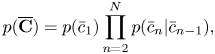
The aim of automatic singing transcription (AST) is to estimate a human-readable musical score of singing voice from a given music signal. Since the melody line is usually the most salient part of music that influences the impression of a song, transcribed scores are useful for music information retrieval (MIR) tasks such as query-by-humming, musical grammar analysis [Reference Hamanaka, Hirata and Tojo1], and singing voice generation [Reference Blaauw and Bonada2]. In this paper, we study statistical audio-to-score (wave-to-MusicXML) AST for audio recordings of popular music consisting of monophonic singing voice and accompaniment sounds (Fig. 1).

Fig. 1. The problem of automatic singing transcription. The proposed method takes as input a spectrogram of a target music signal and tatum times and estimates a musical score of a sung melody.
To estimate the semitone-level pitches and tatum-level onset and offset times of musical notes from music signals, one may estimate a singing F0 trajectory [Reference Bittner, McFee, Salamon, Li and Bello3–Reference Gfeller, Frank, Roblek, Sharifi, Tagliasacchi and Velimirović6] and then quantize it on the semitone and tatum grids obtained by a beat-tracking method [Reference Böck, Korzeniowski, Schlüter, Krebs and Widmer7], where the tatum (e.g. 16th-note level) refers to the smallest meaningful subdivision of the main beat (e.g. fourth-note level). This approach, however, has no mechanism that avoids out-of-scale pitches and irregular rhythms caused by the considerable pitch and temporal variation of the singing voice.
An effective way of overcoming this problem is to use a musical language model that incorporates prior knowledge about symbolic musical scores. Graphical models [Reference Kapanci and Pfeffer8–Reference Nishikimi, Nakamura, Goto, Itoyama and Yoshii11] have been proposed for integrating such a language model with an acoustic model describing the generative process of acoustic features or F0s. In particular, the current state-of-the-art method of audio-to-score AST [Reference Nishikimi, Nakamura, Goto, Itoyama and Yoshii11] is based on a hidden semi-Markov model (HSMM) consisting of a semi-Markov language model describing the generative process of a note sequence and a Cauchy acoustic model describing the generative process of an F0 contour from the musical notes. The semi-Markov model (SMM) is an extension of the Markov model that can explicitly represent the duration probability of each hidden state (e.g. note). While being more accurate than other methods, the output scores include errors caused by the preceding F0 estimation step, and repeated notes of the same pitch cannot be detected from only F0 information. An alternative approach to AST is to use an end-to-end DNN framework to directly convert a sequence of acoustic features into a sequence of musical symbols. At present, however, this approach covers only constrained conditions (e.g. the use of synthetic sound signals) and has only limited success [Reference Carvalho and Smaragdis12–Reference Nishikimi, Nakamura, Goto and Yoshii15].
To solve this problem, we propose an AST method that integrates a language model with a DNN-based acoustic model. This approach can utilize both the statistical knowledge about music notes and the capacity of DNNs for describing complex data distributions of input music signals. This is known as the hybrid approach, which has been one of the major approaches to automatic speech recognition (ASR) [Reference Dahl, Yu, Deng and Acero16]. To our knowledge, the hybrid approach has not been attempted for audio-to-score AST in the literature. The language model describing the generative process of local keys, note pitches, and onset times is implemented with a SMM. The acoustic model describing the generative process of a music audio signal from musical notes is implemented with a convolutional recurrent neural network (CRNN) estimating the pitch and onset probabilities for each tatum. Since the accuracy of beat tracking is already high [Reference Böck, Korzeniowski, Schlüter, Krebs and Widmer7], we assume that beat and downbeat times (i.e. tatum times and their relative metrical positions in measures) are estimated in advance. In this paper, we focus on typical popular songs with 4/4 time. We also investigate how the application of singing voice separation for an input signal affects the transcription results.
The main contributions of this study are as follows. We propose the first DNN-HMM-type hybrid model for audio-to-score AST. The key difference from the HSMM-based method [Reference Nishikimi, Nakamura, Goto, Itoyama and Yoshii11] is that the acoustic model can directly describe complex data distributions of music signals by leveraging the potential of the CRNN. Despite the active research on AST-related tasks like singing voice separation and F0 estimation, a full AST system that can output musical scores in a human-readable form has scarcely been studied. Our system can deal with polyphonic music signals and output symbolic musical scores in the MusicXML format. We found that the proposed method outperformed the HSMM-based method [Reference Nishikimi, Nakamura, Goto, Itoyama and Yoshii11] by a large margin. We also confirmed that the language model significantly improves the AST performance, especially in the rhythm aspects. Finally, we found that the application of singing voice separation to the input music signals can further improve the performanceFootnote 1.
The rest of this paper is as follows: Section II explains backgrounds for the proposed method. Section III describes our approach to AST. Section IV reports the experimental results. Section V concludes the paper.
II. BACKGROUNDS
Before describing the proposed method in the next section, we here explain the backgrounds by reviewing previous studies. Input signal representations have been studied for music information processing, including the short-time Fourier transform (STFT) [Reference Jansson, Humphrey, Montecchio, Bittner, Kumar and Weyde17, Reference Kelz, Dorfer, Korzeniowski, Böck, Arzt and Widmer18], the constant-Q transform (CQT) [Reference Gfeller, Frank, Roblek, Sharifi, Tagliasacchi and Velimirović6], and the log Mel-scale filter-bank [Reference Hawthorne19]. Recently, the harmonic CQT (HCQT) representation, which is obtained by stacking pitch-shifted (upshifted and downshifted) CQT spectrograms, has been proposed [Reference Bittner, McFee, Salamon, Li and Bello3]. This representation was designed to better capture the structure of harmonic partials in music audio signals. Since the HCQT representation is considered to be especially effective for extracting pitch features, we use a similar input representation in our method.
Markov models have widely been used for musical language modeling. To characterize the musical scales, for example, the statistical characteristics of pitch transitions can be learned from musical scores transposed to the C major key [Reference Brooks, Hopkins, Neumann and Wright20]. In automatic music transcription, musical keys are often treated as latent variables instead of referring to key annotations [Reference Nishikimi, Nakamura, Goto, Itoyama and Yoshii11]. As to musical rhythms, SMMs such as the duration-based Markov model [Reference Takeda, Saito, Otsuki, Nakai, Shimodaira and Sagayama21] and the metrical Markov model [Reference Raphael22, Reference Hamanaka, Goto, Asoh and Otsu23] have been proposed. The latter can be used for effectively regularizing the metrical structures of the estimated scores from the rhythmic viewpoint [Reference Nakamura, Yoshii and Sagayama24]. In this study, we construct a Markov model of latent note pitches conditioned by latent musical keys and that of latent note positions.
III. PROPOSED METHOD
We specify the audio-to-score AST problem in Section III-A) and describe the proposed generative modeling approach to this problem in Section III-B). We formulate the CRNN-HSMM model in Sections III-C) and III-E). We explain how to train the model parameters in Section III-F) and the transcription algorithm in Section III-G).
A) Problem specification
We formulate the audio-to-score AST problem under two simplified but practical conditions; (1) The time signature of a target song is $4/4$ ; and (2) the tatum times of the song, which form the 16th note-level grids, are estimated in advance (e.g. [Reference Böck, Korzeniowski, Schlüter, Krebs and Widmer7]).
The input data consist of the audio spectrogram of a target song with tatum times and their relative metrical positions in measures. Similarly to the HCQT representation [Reference Bittner, McFee, Salamon, Li and Bello3], the audio spectrogram is obtained by stacking $H$ pitch-shifted (upshifted and downshifted) versions of a log-frequency magnitude spectrogram obtained by warping the linear frequency axis of the STFT spectrogram into the log-frequency axis. Thus, the input audio spectrogram can be represented as a tensor $\mathbf{X} \in \mathbb{R}^{H\times F\times T}$
 , where $H$
 , $F$
, $F$ , and $T$
 represent the number of channels, that of frequency bins, and that of time frames, respectively.
We use the notation “${}_{i{:}j}$ ” to represent a sequence of integer indices from $i$
 to $j$
 . The tatum times can be represented by a sequence of frame indices $t_{1:{N+1}}$
 , where $n$
 s label tatums, $N$
 is the number of tatums in the input song, and $t_{N+1}$
 indicates a “sentinel” frame of the song. By trimming off unimportant frames before the first tatum and after the last tatum if necessary, we can assume that $t_1=1$
 and $t_{N+1}=T+1$
 . The relative position of tatum $n$
 in a measure is called the metrical position and denoted by $l_n\in \{1,\ldots ,L\}$
 ($L=16$
 is the number of tatums in each measure); $l_n=1$
 means that tatum $n$
 is a downbeat (the first tatum of a measure). In general, we have $l_{n+1}-l_n\equiv 1~(\textrm {mod}\,L)$
 ; however, we do not assume $l_1=1$
 . We use the symbol $m\in \{1,\ldots ,M\}$
 to label measures ($M$
 is the number of measures).
The output of the proposed method is a sequence of musical notes represented by pitches $p_{1:J}$ and onset (score) time in tatum units $n_{1:J+1}$
 . We use the symbol $j$
 to label musical notes, and $J$
 represents the number of estimated musical notes. The pitch $p_j$
 of the $j$
 th note takes a value in $\{0,1,\ldots ,K\}$
 ; $p_j=0$
 means that it is a rest and $p_j>0$
 means that it is a pitched note ($K$
 be the number of unique semitone-level pitches considered). The onset time $n_j$
 of the $j$
 th note takes a value in $\{1,\ldots ,N+1\}$
 and, for convenience, we assume that $n_1=1$
 and $n_{J+1}=N+1$
 . The $(J+1)$
 th note onset is introduced only for defining the length of the $J$
 th note and is not used in the output transcribed score.
For musical language modeling, we introduce musical key variables, which are also estimated in the transcription process. To allow modulations (key changes) within a song, we introduce a local key $s_m$ for each measure $m$
 . Each variable $s_m$
 takes a value in $\{1=\textrm {C},2={\rm C}\sharp ,\ldots ,12=\textrm {B}\}$
 . Since similar musical scales are used in relative major and minor keys, they are not distinguished here. For example, $s_m=0$
 means that measure $m$
 is in the C major key or the A minor key.
B) Generative modeling approach
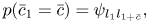
We propose a generative modeling approach to the audio-to-score AST problem (Fig. 2). We formulate a hierarchical generative model of the local keys $\mathbf{S}=s_{1:M}$ , the pitches $\mathbf{P}=p_{1:J}$
 and onset times $\mathbf{N}=n_{1:J+1}$
 of the musical notes, and the spectrogram $\mathbf{X}$
 as
as

Here, all the probabilities are implicitly dependent on the tatum information $t_{1:N+1}$ and $l_{1:N+1}$
 . $p(\mathbf{P}, \mathbf{N}, \mathbf{S})$
 represents a language model that describes the generative process of the musical notes and keys. $p(\mathbf{X} | \mathbf{P}, \mathbf{N})$
 represents an acoustic model that describes the generative process of the spectrogram given the musical notes.
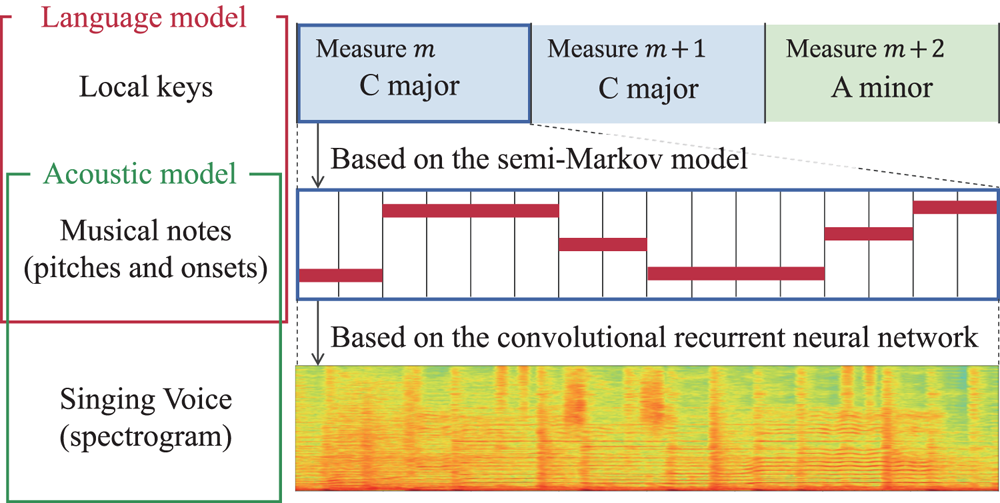
Fig. 2. The proposed hierarchical probabilistic model that consists of a SMM-based language model representing the generative process of musical notes from local keys and a CRNN-based acoustic model representing the generative process of an observed spectrogram from the musical notes. We aim to infer the latent notes and keys from the observed spectrogram.
Given the generative model, the transcription problem can be formulated as a statistical inference problem of estimating the musical scores ($\mathbf{P}, \mathbf{N}$ ) and the keys $\mathbf{S}$
 that maximize the left-hand side of equation (1) for the given spectrogram $\mathbf{X}$
 (as explained later). In this step, the acoustic model evaluates the fitness of a musical score to the spectrogram while the language model evaluates the prior probability of the musical score. The proposed method is therefore consistent with our intuition that both of these viewpoints are essential for transcription.
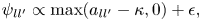
C) Language model
We construct a generative model where the pitches $\mathbf{P}=p_{1:J}$ and the onset times $\mathbf{N}=n_{1:J+1}$
 are independently generated and the pitches are generated depending on the local keys $\mathbf{S}=s_{1:M}$
 . The generative process can be mathematically expressed as

where $p(\mathbf{P}|\mathbf{S})$ , $p(\mathbf{N})$
 , and $p(\mathbf{S})$
 represent the pitch transition model, the onset time transition model, and the key transition model, respectively.
In the key transition model, to represent the sequential dependency between the keys of consecutive measures, the keys $\mathbf{S}=s_{1:M}$ are generated by a Markov model as
The initial and transition probabilities are parameterized as

where we have assumed that the transition probabilities are symmetric under transpositions. For example, the transition probability from C major to D major is assumed to be the same as that from D major to E major. We define ${\boldsymbol \pi} ^\textrm {ini}=(\pi ^\textrm {ini}_s), {\boldsymbol \pi} =(\pi _s)\in \mathbb{R}_{\geq 0}^{12}$ .
.
In the pitch transition model, to represent the dependency of adjacent pitches and the dependency of pitches on the local keys, the pitches $\mathbf{P}=p_{1:J+1}$ are generated by a Markov model conditioned on keys $\mathbf{S}=s_{1:M}$
 as
as
where $m(j)$ indicates the measure to which the $j$
 th note onset belongs. The initial and transition probabilities are parameterized as


We assume that these probabilities are key-transposition-invariant so that the following relations hold:
where
represents the degree (key-relative pitch class) of pitch $p$ in key $s$
 (e.g. $\mathrm {deg}(s,p)=1$
 corresponds to C on the C major scale). We define $\bar{{{\boldsymbol \phi }}}^{\rm ini}\,=\,(\bar{\phi }^{\rm ini}_{d})\,{\in }\,\mathbb{R}_{\geq 0}^{13}$
 and $\bar{{{\boldsymbol \phi }}}\,=\,(\bar{\phi }_{dd'})\,{\in }\,\mathbb{R}_{\geq 0}^{13\times 13}$
 .
.
In the onset time transition model, to represent the rhythmic patterns of musical notes, the onset times $\mathbf{N}=n_{1:J+1}$ are generated by the metrical Markov model [Reference Raphael22, Reference Hamanaka, Goto, Asoh and Otsu23] as
where the initial and transition probabilities are given by
Here, $\delta$ denotes the Kronecker's symbol and the first equation expresses the assumption $n_1=1$
 . In the second equation, ${{\boldsymbol \psi }} = (\psi _{l'l}) \in \mathbb{R}_{\geq 0}^{L\times L}$
 represents the transition probabilities between metrical positions.
D) Tatum-level language model formulation
In the language model presented in Section III-C), the transitions of keys and transitions of pitches and onset times are not synchronized. To enable the integration with the acoustic model and the inference for AST, we here formulate an equivalent language model where the variables are defined at the tatum level. For this purpose, we introduce tatum-level key variables $\bar{s}_n$ , pitch variables $\bar{p}_n$
 , and counter variables $\bar{c}_n$
 (Fig. 3). The first two sets of variables are constructed from the keys $s_{1:M}$
 and the pitches $p_{1:J}$
 so that $\bar{s}_n=s_m$
 when tatum $n$
 is in measure $m$
 and $\bar{p}_n=p_j$
 when tatum $n$
 satisfies $n_j\leq n < n_{j+1}$
 . The counter variable $\bar{c}_n$
 represents the residual duration of the current musical note in tatum units and takes a value in $\{1,\ldots ,2L\}$
 , where $2L$
 is the maximum length of a musical note. This variable is gradually decremented tatum by tatum until the next note begins; a note onset at tatum $n$
 is indicated by $\bar{c}_{n-1}=1$
 . In this way, we can construct variables $\overline {\mathbf{S}}=\bar{s}_{1:N}$
 , $\overline {\mathbf{P}}=\bar{p}_{1:N}$
 , and $\overline {\mathbf{C}}=\bar{c}_{1:N}$
 from variables $\mathbf{S}=s_{1:M}$
 , $\mathbf{P}=p_{1:J}$
 , and $\mathbf{N}=n_{1:J+1}$
 , and vice versa.
Fig. 3. Representation of a melody note sequence and variables of the language model.
The generative models for the tatum-level keys, pitches, and counters can be derived from the language model in Section III-C) as follows. The keys $\overline {\mathbf{S}}=\bar{s}_{1:N}$ obey the following Markov model:
where


The second equation says that a key transition occurs only at the beginning of a measure.
The counters $\overline {\mathbf{C}}=\bar{c}_{1:N}$ obey the following Markov model:
where
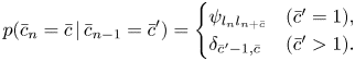
This is a kind of SMM called the residential-time Markov model [Reference Yu25]. As shown in Fig. 3, at the onset tatums of musical notes, the counter variables change to the corresponding note values. Otherwise, the counter variables are decremented by one. The former case is represented by $\psi _{l_{n}l_{n+\bar{c}}}$ and the latter case is represented by $\delta _{\bar{c}' - 1, \bar{c}}$
 in equation (20).
The pitches $\overline {\mathbf{P}}=\bar{p}_{1:N}$ obey the following Markov model conditioned on the keys and counters:
where
The second equation expresses the constraint that a pitch transition occurs only at a note onset.
Putting equations (15), (18), and (21) together, we have

That is, the language model in Section III-C) and the tatum-level language model defined here are equivalent probabilistic models. We use this tatum-level SMM in what follows.
E) Acoustic model
We formulate an acoustic model $p(\mathbf{X} | \mathbf{P}, \mathbf{N})=p(\mathbf{X}|\overline {\mathbf{P}},\overline {\mathbf{C}})$ that gives the probability of spectrogram $\mathbf{X}$
 given a pitch sequence $\overline {\mathbf{P}}$
 and a counter sequence $\overline {\mathbf{C}}$
 representing onset times. We define the tatum-level spectra $\mathbf{X}_n$
 as a segment of spectrogram $\mathbf{X}$
 in the span of tatum $n$
 . As in the standard HMM, we assume the conditional independence of the probabilities of tatum-level spectra as
Using Bayes’ theorem, the individual factors in the right-hand side of equation (25) can be written as
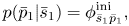
where $p(\bar{p}_n,\bar{c}_{n-1})$ is the prior probability of pitch $\bar{p}_n$
 and counter $\bar{c}_{n-1}$
 and $p(\bar{p}_n, \bar{c}_{n-1}|\mathbf{X}_n)$
 is the posterior probability of $\bar{p}_n$
 and $\bar{c}_{n-1}$
 .
.
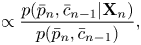
We use a CRNN for estimating the probability $p(\bar{p}_n, \bar{c}_{n-1}|\mathbf{X}_n)$ (Fig. 4). Since it is considered to be difficult to directly estimate the counter variables describing the durations of musical notes from the locally observed quantity $\mathbf{X}_n$
 , we train the CRNN to predict the probability whether a note onset occurs at each tatum. A similar DNN for joint estimation of pitch and onset probabilities has been successfully applied to piano transcription [Reference Hawthorne19]. For reliable estimation, we estimate the pitch and onset probabilities independently. Therefore, the CRNN takes the spectra $\mathbf{X}_n$
 as input and outputs the following probabilities:
where $\bar{o}_n \in \{0, 1\}$ is an onset flag and $\zeta _n$
 is the (posterior) onset probability at tatum $n$
 ($\bar{o}_n = 1$
 if there is a note onset at tatum $n$
 and $\bar{o}_n = 0$
 otherwise). The counter probabilities are assigned using the onset probability as
and the probability $p(\bar{p}_n,\bar{c}_{n-1}|\mathbf{X}_n)$ is then given as the product of equations (28) and (30).
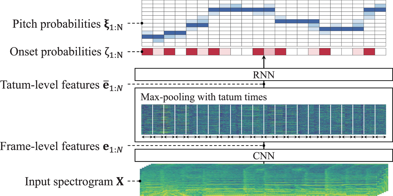
Fig. 4. The acoustic model $p(\mathbf{X} | \overline {\mathbf{P}}, \overline {\mathbf{C}})$ representing the generative process of the spectrogram $\mathbf{X}$
 from note pitches $\overline {\mathbf{P}}$
 and residual durations $\overline {\mathbf{C}}$
 .
.
In practice, it is reasonable to use spectra of a longer segment than a tatum as input of the CRNN since each tatum (16th note) spans a short time interval. In addition, it is computationally efficient to jointly estimate the pitch and onset probabilities of all tatums in the wide segment. Therefore, we use the whole spectrogram $\mathbf{X}$ (or its part of a sufficient duration) as the input of the CRNN and train it so as to output all the tatum-level pitch and onset probabilities.
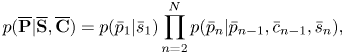
The CRNN consists of a frame-level CNN and a tatum-level RNN linked through a max-pooling layer (Fig. 4). The CNN extracts latent features $\mathbf{e}_{1:T}$ ($\mathbf{e}_t = [e_{t1},\ldots ,e_{tF}] \in \mathbb{R}^{F}$
 ) from the spectrogram $\mathbf{X}$
 of length $T$
 :
:
Using the tatum times $t_{1:N+1}$ , the max-pooling layer summarizes the frame-level features $\mathbf{e}_{1:T}$
 into the tatum-level features $\bar{\mathbf{e}}_{1:N}$
 ($\bar{\mathbf{e}}_{n} =[\bar{e}_{n1},\ldots ,\bar{e}_{nF}] \in \mathbb{R}^{F}$
 ) as
) as
The RNN then converts the tatum-level features $\bar{\mathbf{e}}_{1:N}$ into intermediate features $\mathbf{g}_{1:N}$
 ($\mathbf{g}_n \in \mathbb{R}^{D}$
 is a $D$
 -dimensional vector) through a bidirectional long short-term memory (BLSTM) layer and predicts the pitch and onset probabilities ${\boldsymbol \xi} _{n} = (\xi _{nk})\in \mathbb{R}^{K+1}$
 and $\zeta _n$
 through softmax and sigmoid layers as follows:


where $\mathbf{W}^{\rm p}\in \mathbb{R}^{(K+1) \times D}$ and $\mathbf{W}^{\rm o}\in \mathbb{R}^{1 \times D}$
 are weight matrices, and $\mathbf{b}^{\rm p}\in \mathbb{R}^{K+1}$
 and $b^{\rm o}\in \mathbb{R}$
 are bias parameters.
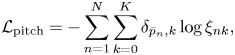
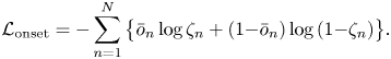
F) Training model parameters
The parameters ${{\boldsymbol \psi }}$ , $\bar{{{\boldsymbol \phi }}}^{\rm ini}$
 , $\bar{{{\boldsymbol \phi }}}$
 , ${{\boldsymbol \pi }}^{\rm ini}$
 , and ${{\boldsymbol \pi }}$
 of the language model are learned from training data of musical scores. The metrical transition probabilities $\psi _{ll'}$
 are estimated as
where $a_{ll'}$ is the number of transitions from metrical positions $l$
 to $l'$
 appear in the training data, $\kappa$
 is a discount parameter, and $\epsilon$
 is a small value to avoid the zero count. The initial and transition probabilities of pitches ($\bar{{{\boldsymbol \phi }}}^{\rm ini}$
 and $\bar{{{\boldsymbol \phi }}}$
 ) are estimated in the same way, by using the key signatures. Although the initial and transition probabilities of local keys (${{\boldsymbol \pi }}^{\rm ini}$
 and ${{\boldsymbol \pi }}$
 ) can be trained in the same way in principle, a large amount of musical scores are necessary for reliable estimation since modulations are rare. Therefore, in this study, we manually set ${{\boldsymbol \pi }}^{\rm ini}$
 to the uniform distribution and ${{\boldsymbol \pi }}$
 to $[0.9, 0.1/11, \ldots , 0.1/11]$
 such that the self-transition probability $\pi _{1}$
 has a large value.
The parameters of the CRNN are trained by using paired data of audio spectrograms and corresponding musical scores. After converting the pitches and onset times into the form $\overline {\mathbf{P}}=\bar{p}_{1:N}$ and $\overline {\mathbf{O}}=\bar{o}_{1:N}$
 , we apply the following cross-entropy loss functions to train the CRNN:
G) Transcription algorithm
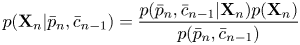
We can derive a transcription algorithm based on the constructed generative model. Using the tatum-level formulation, equation (1) can be rewritten as

where the first factor on the right-hand side is given by the CRNN as in equation (25) and the second factor by the SMM as in equation (24). Therefore, the integrated generative model is a CRNN-HSMM hybrid model. The most likely musical score can be estimated from the observed spectrogram $\mathbf{X}$ by maximizing the probability $p(\overline {\mathbf{S}},\overline {\mathbf{P}},\overline {\mathbf{C}}|\mathbf{X})\propto p(\mathbf{X},\overline {\mathbf{S}},\overline {\mathbf{P}},\overline {\mathbf{C}})$
 , where we have used Bayes’ formula. In equation, we estimate the optimal keys $\overline {\mathbf{S}}^{*}=\bar{s}^{*}_{1:N}$
 , pitches $\overline {\mathbf{P}}^{*}=\bar{p}^{*}_{1:N}$
 , and counters $\overline {\mathbf{C}}^{*}=\bar{c}^{*}_{1:N}$
 at the tatum level such that

The most likely pitches $\mathbf{P}^{*}=p^{*}_{1:J}$ and onset times $\mathbf{N}^{*}=n^{*}_{1:J}$
 of musical notes can be obtained from $\overline {\mathbf{P}}^{*}$
 and $\overline {\mathbf{C}}^{*}$
 . The number of notes $J$
 is determined in this inference process.
1) Viterbi Algorithm
We can use the Viterbi algorithm to solve equation (40). In the forward step, Viterbi variables $\omega _n (q_n)$ , where $q_n = \left \{\bar{s}_n, \bar{p}_n, \bar{c}_n\right \}$
 , are recursively calculated as follows:
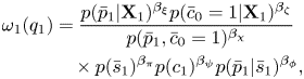
where $\bar{c}_0=1$ was formally introduced in the initialization. In the above equations, we have introduced weighting factors $\beta _{\pi }$
 , $\beta _{\phi }$
 , $\beta _{\psi }$
 , $\beta _{\xi }$
 , $\beta _{\zeta }$
 , and $\beta _{\chi }$
 to balance the language model and the acoustic model. In the recursive calculation, $q_{n-1}$
 that maximizes the max operation is memorized as $\mathrm {prev}(q_n)$
 .
.
In the backward step, the optimal variables $q^{*}_{1:N}$ are recursively obtained as follows:
2) Refinements
Musical scores estimated by the CRNN-HSMM tend to have long durations because the accumulative multiplication of pitch and onset time transition probabilities decreases the posterior probability. This is known as a general problem of the HSMM [Reference Nishikimi, Nakamura, Goto, Itoyama and Yoshii11]. To ameliorate this situation, we penalize long notes by multiplying each of equations (41) and (42) by the following penalty term:
where $\beta _{\eta } \ge 0$ is a weighting factor.
To save the computational costs of the Viterbi algorithm defined in the large product space $q_n=\{\bar{s}_n,\bar{p}_n,\bar{c}_n\}$ without sacrifice of its global optimality, we limit the pitch space to be searched as follows:
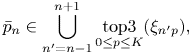
where $\mathrm {top3}_{0\leq p\leq K}(\xi _{np})$ represents the set of the indices $p$
 that provide the three largest elements in $\{\xi _{n0},\ldots ,\xi _{nK}\}$
 .
.
IV. EVALUATION
We report comparative experiments conducted for evaluating the proposed AST method. We compared the proposed method with existing methods and examined the effectiveness of the language model (Section IV-C)). We then investigated the AST performance of the proposed method for music and singing signals with different complexities and examined the influence of the beat tracking performance on the AST performance (Section IV-D)).
A) Data
We used $61$ popular songs with reliable melody annotations [Reference Goto26] from the RWC Music Database [Reference Goto, Hashiguchi, Nishimura and Oka27]. We split the data into a training dataset ($37$
 songs), a validation dataset ($12$
 songs), and a test dataset ($12$
 songs), where the singers of these datasets are disjoint. We also used 20 synthesized singing signals obtained by a singing synthesis software called CeVIO [28]; $12$
 , $4$
, $4$ , and $4$
 signals are added to the training, validation, and test datasets, respectively.
To augment the training data for the acoustic model, we added the separated singing signals obtained by Spleeter [Reference Hennequin, Khlif, Voituret and Moussallam29] and the clean isolated singing signals. To cover a wide range of pitches and tempos, we pitch-shifted the original music signals by $L$ semitones ($-12 \le L \le 12$
 ) and randomly time-stretched each of those signals with a ratio of $R$
 ($0.5 \le R < 1.5$
 ). The total number of songs in the training data was $37 \times 25 \times 3 \text { (real)} + 49 \times 25 \text { (synthetic)}= 4000$
 . Since the initial and transition probabilities of pitches are key-transposition-invariant, the pitch shifting does not affect the training of those probabilities. Therefore, we did not apply data augmentations for training the language model.
For each signal sampled at $22.05$ kHz, we used a STFT with a Hann window of $2048$
 points and a shifting interval of $256$
 points ($11.6$
 ms) for calculating the amplitude spectrogram on the logarithmic frequency axis having $5$
 bins per semitone (i.e. $1$
 bin per $20$
 cents) between $32.7$
 Hz (C1) and $2093$
 Hz (C7) [Reference Cheuk, Anderson, Agres and Herremans30]. We then computed the HCQT-like spectrogram $\mathbf{X}$
 by stacking the $h$
 -harmonic-shifted versions of the original spectrogram, where $h \in \{1/2,1,2,3,4,5\}$
 (i.e. $H=6$
 ), and the lowest and highest frequencies of the $h$
 -harmonic-shifted spectrogram are $h \times 32.7$
 Hz and $h \times 2093$
 Hz, respectively.
B) Setup
Inspired by the CNN proposed for frame-level melody F0 estimation [Reference Bittner, McFee, Salamon, Li and Bello3], the frame-level CNN of the acoustic model (Fig. 5) was designed to have six convolution layers with the output channels of $128$ , $64$
 , $64$
 , $64$
 , $8$
, $8$ , and $1$
 and the kernel sizes of $(5,5)$
 , $(5,5)$
 , $(3,3)$
 , $(3,3)$
 , $(70,3)$
 , and $(1,1)$
 , respectively, where the instance normalization [Reference Ulyanov, Vedaldi and Lempitsky31] and the Mish function [Reference Misra32] are used. The output dimension of the tatum-level BLSTM was set to $D = 130 \times 2$
 . The vocabulary of pitches consisted of a rest and $128$
 semitone-level pitches specified by the MIDI note numbers ($K=128$
 ).
).
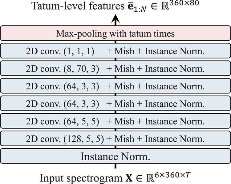
Fig. 5. Architecture of the CNN. Three numbers in the parentheses in each layer indicate the channel size, height, and width of the kernel.
To optimize the proposed CRNN, we used RAdam with the parameters $\alpha = 0.001$ (learning rate), $\beta _1=0.9$
 , $\beta _2=0.999$
 , and $\varepsilon =10^{-8}$
 . A weight decay (L2 regularization) with a hyperparameter $10^{-5}$
 and a gradient clipping with a threshold of $5.0$
 were used for training. The weight parameters $\mathbf{W}^\textrm {p}$
 and $\mathbf{W}^\textrm {o}$
 were initialized to random values between $-0.1$
 and $0.1$
 . The kernel filters of the frame-level CNN and the weight parameters of the tatum-level BLSTM were initialized by He's method [Reference He, Zhang, Ren and Sun33]. All bias parameters were initialized with zero.
Because of the limited memory capacity, we split the spectrogram of each song into 80-tatum segments. The CRNN's outputs of those segments were concatenated for the note estimation based on the Viterbi decoding. The weighting factors $\beta _{\pi }$ , $\beta _{\phi }$
 , $\beta _{\psi }$
 , $\beta _{\xi }$
 , $\beta _{\zeta }$
 , and $\beta _{\eta }$
 were optimized for the validation data by using Optuna [Reference Akiba, Sano, Yanase, Ohta and Koyama34]. Consequently, $\beta _{\pi }=0.541$
 , $\beta _{\phi }=0.769$
 , $\beta _{\psi }=0.619$
 , $\beta _{\xi }=0.917$
 , $\beta _{\zeta }=0.852$
 , and $\beta _{\eta }=0.609$
 . We manually set the weighting factor $\beta _\chi$
 to $0$
 based on the results of preliminary experiments. The discounting value $\kappa$
 and small value $\epsilon$
 in equation (36) were set to $0.7$
 and $0.1$
 , respectively.
The accuracy of estimated musical notes was measured with the edit-distance-based metrics proposed in [Reference Nakamura, Yoshii and Sagayama24] consisting of pitch error rate ${E_{\rm p}}$ , missing note rate ${E_{\rm m}}$
 , extra note rate ${E_{\rm e}}$
 , onset error rate ${E_{\rm on}}$
 , offset error rate ${E_{\rm off}}$
 , and overall (average) error rate ${E_{\rm all}}$
 .
.
C) Method comparison
To confirm the AST performance of the proposed method, we compared the transcription results obtained by the proposed CRNN-HSMM hybrid model, the HHSMM-based method [Reference Nishikimi, Nakamura, Goto, Itoyama and Yoshii11], and the majority-vote method. The majority-vote method quantizes an input F0 trajectory in semitone units, then determines tatum-level pitches by taking the majority of the quantized pitches at each tatum. Since the majority-vote method does not estimate note onsets, we concatenated successive tatums with the same pitch to obtain a single musical note. The HHSMM-based method does not estimate rests because it is difficult to model the unvoiced frames in an F0 contour. To obtain rests from the musical score estimated by the HHSMM-based method, we removed the estimated musical notes if the unvoiced frames occupied 90% and more of each musical note.
To examine the effect of the language model, we also run a method using only the CRNN as follows:
To construct a musical score from the predicted symbols $p^{*}_n$ and $o^{*}_n$
 , we applied the following rules:
(i) If $p^{*}_{n-1} \neq p^{*}_n$
 , then the $(n-1)$ th and $n$ th tatums are included in different notes.
(ii) If $p^{*}_{n-1} = p^{*}_n$
and $o^{*}_n = 1$, then the $(n-1)$ th and $n$ th tatums are included in different notes having the same pitch.(iii) If $p^{*}_{n-1} = p^{*}_n$
and $o^{*}_n = 0$, then the $(n-1)$ th and $n$ th tatums are included in the same notes.


To evaluate the methods in a realistic situation, only the mixture signals and the separated signals were used as test data, and the tatum times were estimated by [Reference Böck, Korzeniowski, Schlüter, Krebs and Widmer7].
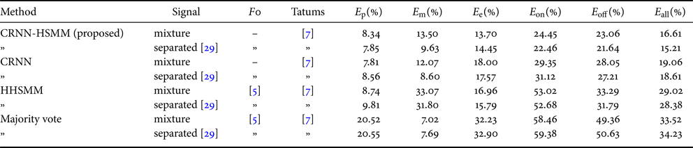
Results are shown in Table 1. For both the mixture and separated signals, the proposed method and the CRNN method outperformed the majority-vote method and the HHSMM-based method in the overall error rate $E_\textrm {all}$ by large margins. This result confirms the effectiveness of using the CRNN as the acoustic model. Comparing the $E_\textrm {all}$
 metrics for the proposed method and the CRNN method, there was a decrease of $2.33$
 percentage points (PP) for the mixture signals and $1.62$
 PP for the separated signals. This result indicates the positive effect of the language model. Especially, the significant decreases of the $E_\textrm {on}$
 and $E_\textrm {off}$
 metrics indicate that the language model is particularly effective for reducing rhythm errors. The proposed method and the CRNN method achieved better performances for the separated signals than the mixture signals.
Table 1. The AST performances of the different methods.
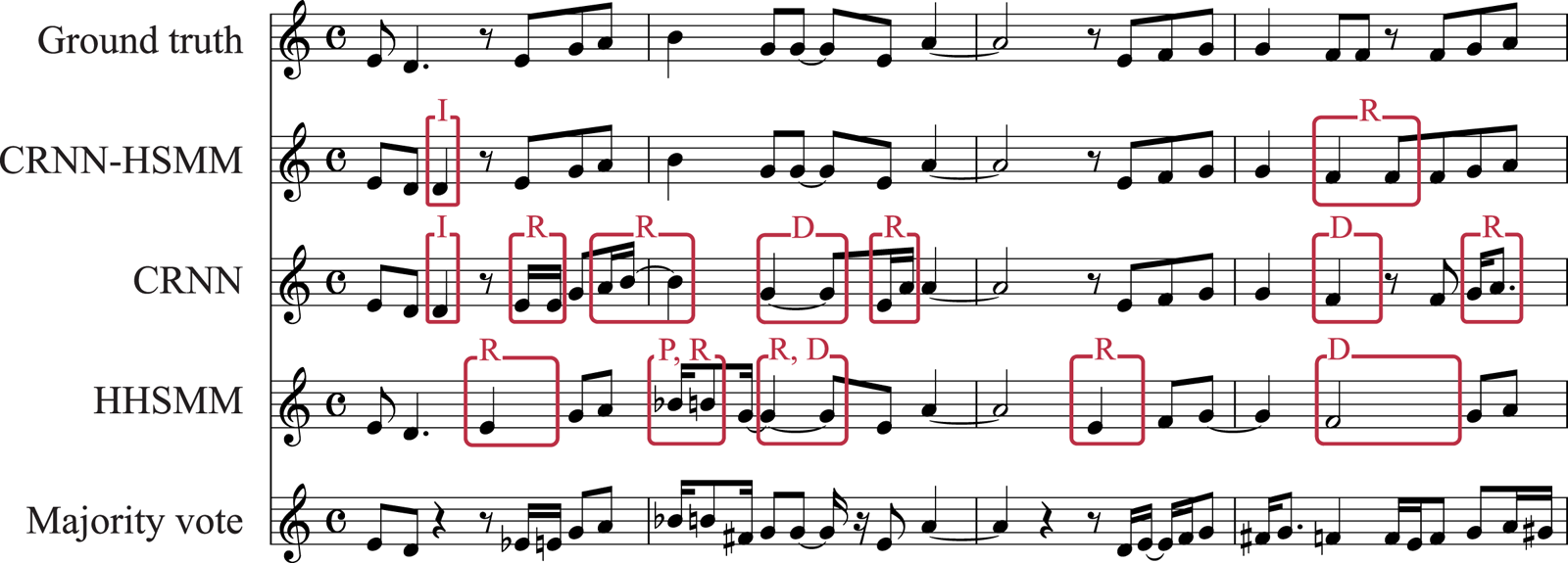
Transcription examples obtained by the different models are shown in Fig. 6 Footnote 2. The musical score estimated by the majority-vote method, which did not use a language model, had many errors. In the musical score estimated by the HHSMM-based method, whereas most notes had pitches on the musical scale, repeated note onsets with the same pitches were not detected. In the result by the CRNN method, which did not use a language model, we can see that most pitches are on the musical scale unlike in the result by the majority-vote method. This indicates the capacity of the CRNN that some sequential constraints on musical notes can be learned by the RNN. However, there were some errors in rhythms, which suggests the difficulty of learning rhythmic constraints by a simple RNN. Finally, in the result by the proposed CRNN-HSMM method, there were much fewer rhythm errors than the CRNN method, which demonstrates the effect of the language model. The transition probabilities $\bar{{{\boldsymbol \phi }}}$ and ${{\boldsymbol \psi }}$
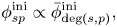
 are shown in Fig. 7. Figure 7(a) shows that the transitions to the seven pitch classes on the C major scale tend to occur frequently. Figure 7(b) shows that the transitions to the 8th-note-level metrical positions tend to occur frequently.

Fig. 6. Examples of musical scores estimated by the proposed method, the CRNN method, the HHSMM-based method, and the majority-vote method from the separated audio signals and the estimated F0 contours and tatum times. Transcription errors are indicated by the red squares. Capital letters attached to the red squares represent the following error types: pitch error (P), rhythm error (R), deletion error (D), and insertion error (I). Error labels are not shown in the transcription result by the majority-vote method, which contains too many errors.
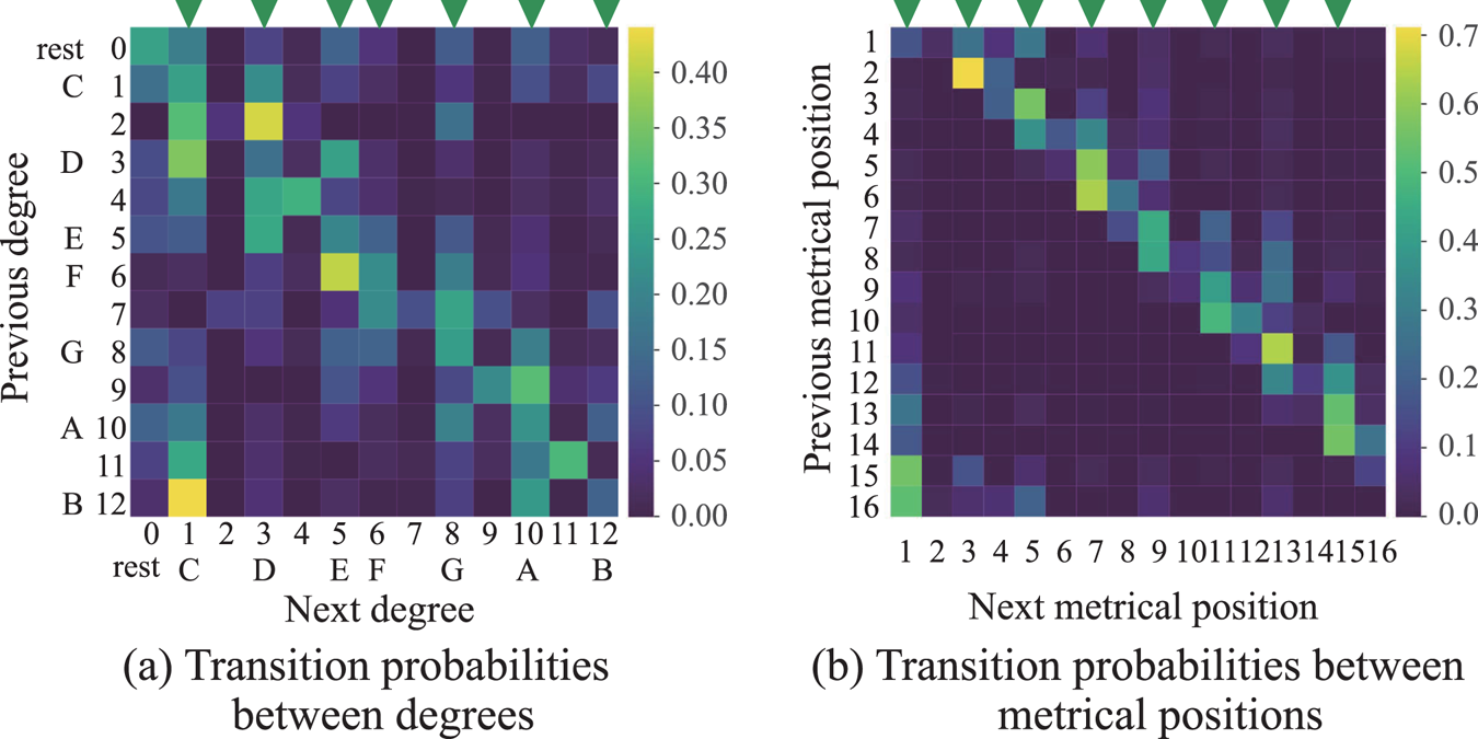
Fig. 7. The transition probabilities $\bar{{{\boldsymbol \phi }}}$ and ${{\boldsymbol \psi }}$
 trained from the existing musical scores. The triangles indicate (a) the seven pitch classes on the C major scale and (b) the eighth-note-level metrical positions.
The end-to-end approaches to AST based on sequence-to-sequence (seq2seq) learning have been studied [Reference Carvalho and Smaragdis12, Reference Román, Pertusa and Calvo-Zaragoza13]. The RNN-based method [Reference Carvalho and Smaragdis12] and the CTC-based method [Reference Román, Pertusa and Calvo-Zaragoza13] achieved low error rates (e.g. $P(sub) = 0.006$ and ${E_{\rm p}}=0.99\%$
 ) for synthetic signals. Similarly, as shown in Table 2, the proposed method also achieved low error rates (e.g. ${E_{\rm p}}=0.42\%$
 ) for synthetic singing voices. Note that these methods were not evaluated on the same real data we used.
Table 2. The AST performances obtained from the different input data.

D) Influences of voice separation and beat tracking methods
A voice separation method [Reference Hennequin, Khlif, Voituret and Moussallam29] and a beat-tracking method [Reference Böck, Korzeniowski, Schlüter, Krebs and Widmer7] are used in the preprocessing step of the proposed method, and errors made in this step can propagate to the final transcription results. Here, we investigate the influences of those methods used in the preprocessing step. We used the ground-truth tatum times obtained from the beat annotations [Reference Goto26] to examine the influence of the beat-tracking method. We used the isolated signals for the songs in the test data to examine the influence of the voice separation method. In addition, as a reference, we also evaluated the proposed method with the synthetic singing voices. When tatum times were estimated by the beat-tracking method [Reference Böck, Korzeniowski, Schlüter, Krebs and Widmer7] for the real signals, the mixture signals are used as input and the results are used for the mixture, separated, and isolated signals. Since the synthesized signals are not synchronized to the mixture signals, the beat-tracking method is directly applied to the vocal signals to obtain estimated tatum times.
Results are shown in Table 2. As for the influence of the beat-tracking method, using the ground-truth tatum times decreased the overall error rate $E_\textrm {all}$ by $1.1$
 PP for the separated signals and $1.3$
 PP for the isolated signals. This result indicates that the influence of the beat-tracking method is small for the data used. As for the influence of the voice separation method, in both conditions with estimated and ground-truth tatum times, $E_\textrm {all}$
 for the isolated signals were approximately $3$
 PP smaller than that for the separated signals. This result indicates that further refinements on the voice separation method can improve the transcription results by the proposed method.
Although the singing voice separation had both the positive and negative impacts, as a whole, it improved the transcription performances in most metrics. Especially, the missing note rates were decreased by $5.4$ PP and $3.9$
 PP when the ground-truth and estimated tatum times were used, respectively. However, the pitch error rates and the extra note rates were increased when the ground-truth and estimated tatum times were used, respectively. In addition, the performance gain obtained for the separated signals was smaller than that for the isolated signals. Figure 8 shows transcription examples obtained for mixture and separated signals with the ground-truth tatum times. In the left figure, the extra notes were eliminated successfully by suppressing the accompaniment sounds. In the right figure, in contrast, the residual accompaniment sounds were wrongly recognized as melody notes.
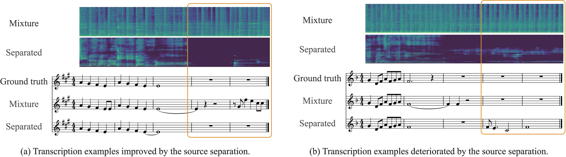
Fig. 8. Examples of musical scores obtained with and without singing voice separation when the ground-truth tatum times were used. The left and right figures illustrate the positive and negative impacts of singing voice separation.
Finally, in both conditions with estimated and ground-truth tatum times, the transcription error rates for the synthesized signals were significantly smaller than those for the real signals. This result confirms that the difficulty of AST originates from the pitch and timing deviations in sung melodies. The relatively large onset and offset error rates for the case of using the estimated tatum times are due to the difficulty of beat tracking for the signals containing only a singing voice.
E) Discussion
Our results provide an important insight that a simple RNN has a weak effect in capturing the rhythmic structure and the language model that explicitly incorporates a rhythm model plays a significant role in improving the transcription results. Whereas musical pitches can be inferred from local acoustic features, in order to recognize musical rhythms, it is necessary to look at durations or intervals of onset times, which have extended structures in time. This non-local feature of rhythms characterizes the difficulty of music transcription, which cannot be solved by simply applying DNN techniques used for other tasks such as ASR. This result may also explain why end-to-end methods that were successful at ASR have not been so successful at music transcription [Reference Carvalho and Smaragdis12–Reference Nishikimi, Nakamura, Goto and Yoshii15]. For example, the paper [Reference Román, Pertusa and Calvo-Zaragoza13] reports low error rates for monophonic transcription, but the method was only applied to synthetic data without timing deviations.
To simplify the AST task, we imposed the following restrictions on target songs in this study: the tatum unit (minimal resolution of a beat) is a 16th-note length and the meter of a target song is 4/4 time. Theoretically, we can relax these restrictions by modifying the language model and extend the present method for more general target songs. To include shorter note lengths and triplets, we can introduce a shorter tatum unit, for example, a tatum corresponding to one-third of a 32nd note. To transcribe songs in other meters such as 3/4 time, we can construct one metrical Markov model for each meter and estimate the meter of a given song by the maximum likelihood estimation [Reference Nakamura, Yoshii and Sagayama24]. Although most beat-tracking methods such as [Reference Böck, Korzeniowski, Schlüter, Krebs and Widmer7] assumes a constant meter for each song, popular music songs often have mixed meters (e.g. an insertion of a measure in 2/4 time), which calls for a more general rhythm model. A possible solution is to introduce latent variables representing meters (one for each measure) into the language model and estimate the variables in the transcription step.
The language model based on the first-order Markov model was used in this study and it is possible to apply more refined language models. A simple direction is to use higher-order Markov models or a neural language model based on RNN. While most language models try to capture local sequential dependence of symbols, using a model incorporating a global repetitive structure is effective for music transcription. To incorporate the repetitive structure in a computationally tractable way, it is considered to be effective to use a Bayesian language model [Reference Nakamura, Itoyama and Yoshii35].
Another important direction for refining the method would be to integrate the voice separation and/or the beat tracking with the musical note estimation method. A voice separation method and a beat-tracking method are used in the preprocessing step in the present method, and we observed that errors made in the preprocessing step can propagate to the transcription results. To mitigate the problem, multi-task learning of the singing voice separation and the AST can also be effective in obtaining the singing voices appropriate for the AST [Reference Nakano, Yoshii, Wu, Nishikimi, Edward Lin and Goto5]. A beat-tracking method typically estimates beat times in the accompaniment sounds, which can be slightly shifted from the onset times of the singing voice due to the asynchrony between the vocal and the other parts [Reference Nishikimi, Nakamura, Goto, Itoyama and Yoshii36]. Therefore, it would be effective for AST to jointly estimate musical notes and tatum times that match the onset times of singing voices.
V. Conclusion
This paper presented an audio-to-score AST method based on a CRNN-HSMM hybrid model that integrates a language model with a DNN-based acoustic model. The proposed method outperformed the majority-vote method and the previously state-of-the-art HHSMM-based method. We also found that the language model has a positive effect on improving the AST performance, especially in rhythmic aspects.
The proposed approach of integrating the SMM-based language model with the DNN-based acoustic model is a general framework that can be applied to other tasks of music transcription such as chord estimation, music structure analysis, and instrumental music transcription. It would be interesting to investigate how the proposed method works on genres other than popular music. Another interesting possibility is to integrate language models [Reference Ojima, Nakamura, Itoyama and Yoshii37, Reference Nakamura and Yoshii38] and acoustic models [Reference Hawthorne19, Reference Kim and Bello39] that can deal with chords for polyphonic piano transcription. Eventually, based on the proposed framework, we aim to build a unified audio-to-score transcription system that can estimate musical scores of multiple parts of popular music.
FINANCIAL SUPPORT
This work was partially supported by JSPS KAKENHI Nos. 16H01744, 19H04137, 19K20340, 19J15255, and 20K21813, and JST ACCEL No. JPMJAC1602 and PRESTO No. JPMJPR20CB.
CONFLICT OF INTEREST
None.
Ryo Nishikimi received the B.E. and M.S. degrees from Kyoto University, Kyoto, Japan, in 2016 and 2018, respectively. He is currently working toward the Ph.D. degree in Kyoto University, and has been a Research Fellow of the Japan Society for the Promotion of Science (DC2). His research interests include music informatics and machine learning. He is a student member of IEEE and IPSJ.
Eita Nakamura received a Ph.D. degree in physics from the University of Tokyo in 2012. He has been a post-doctoral researcher at the National Institute of Informatics, Meiji University, and Kyoto University. He is currently an Assistant Professor at the Hakubi Center for Advanced Research and Graduate School of Informatics, Kyoto University. His research interests include music modelling and analysis, music information processing and statistical machine learning.
Masataka Goto received the Doctor of Engineering degree from Waseda University in 1998. He is currently a Prime Senior Researcher at the National Institute of Advanced Industrial Science and Technology (AIST), Japan. Over the past 28 years he has published more than 270 papers in refereed journals and international conferences and has received 51 awards, including several best paper awards, best presentation awards, the Tenth Japan Academy Medal, and the Tenth JSPS PRIZE. In 2016, as the Research Director he began OngaACCEL Project, a 5-year JST-funded research project (ACCEL) on music technologies.
Kazuyoshi Yoshii received the M.S. and Ph.D. degrees in informatics from Kyoto University, Kyoto, Japan, in 2005 and 2008, respectively. He is an Associate Professor at the Graduate School of Informatics, Kyoto University, and concurrently the Leader of the Sound Scene Understanding Team, Center for Advanced Intelligence Project (AIP), RIKEN, Tokyo, Japan, and the Researcher of PRESTO, Japan Science and Technolocy Agency (JST), Tokyo, Japan. His research interests include music informatics, audio signal processing, and statistical machine learning.


 Open access