


1. Introduction
Particle-laden flows play an important role in today's world due to the large number of industrial applications relying on them. These kind of flows are characterized by numerous solid–solid contacts, either particle–particle or particle–wall contacts. All these solid–solid interactions can electrically charge the solid phase via the triboelectric effect (Forward Reference Forward2009). These electrically charged particles can now interact with each other due to the Lorentz force. However, because the particle's velocity is much smaller than the speed of light, the only relevant component is the electrostatic force.
For simplicity reasons, this electrostatic force is generally neglected in mathematical modelling approaches and numerical simulations. However, it is well known that the electrostatic effects are at the root of several problems in many industrial reactors, especially in fluidized beds. Due to their different electrical polarity, particles might get attached to the reactor's wall. This greatly diminishes the solid mixing and could even force the complete shutdown of the reactor (Hendrickson Reference Hendrickson2006). In addition to this, the electrostatic force can also modify important dynamic properties of the reactor such as: bubble size (Dong et al. Reference Dong, Zhang, Huang, Liao, Wang and Yang2015), minimum fluidization velocity (Manafi, Zarghami & Mostoufi Reference Manafi, Zarghami and Mostoufi2019), heat transfer coefficient (Miller & Logwinuk Reference Miller and Logwinuk1951) and fine entrainment rate (Baron et al. Reference Baron, Briens, Bergougnou and Hazlett1987).
In recent years, some efforts have been directed towards developing predictive mathematical tools capable of modelling the effect of this force in gas–solid flows (Chowdhury et al. Reference Chowdhury, Ray, Sowinski, Mehrani and Passalacqua2021). Rokkam, Fox & Muhle (Reference Rokkam, Fox and Muhle2010) and Rokkam et al. (Reference Rokkam, Sowinski, Fox, Mehrani and Muhle2013) were among the first to propose the use of an Eulerian approach for a fluidized bed with electrostatic forces. Using a model where the particles have a constant electric charge, they were able to reproduce the wall sheeting effects in a fluidized bed reactor. However, the constant electric charge assumption might be very restrictive as it cannot account for the effects due to the electric charge spatial distribution. In addition to this, it would require previous knowledge of the solid phase electric charge. To solve this limitation, Kolehmainen, Ozel & Sundaresan (Reference Kolehmainen, Ozel and Sundaresan2018b) suggested deriving a full transport equation for the particle electric charge in the framework of the kinetic theory of granular rapid flow. However, this approach is known to require closure law models for the higher-order moments, such as the particle-velocity covariance and the charge variance. Multiple strategies are possible to overcome this problem. One can neglect them altogether (Ceresiat, Kolehmainen & Ozel Reference Ceresiat, Kolehmainen and Ozel2021). A first-order approximation can be made by making an analogy with the heat transfer coefficient (Kolehmainen et al. Reference Kolehmainen, Ozel and Sundaresan2018b). Finally, a more rigorous strategy consists of deriving algebraic models obtained by simplifying the second-order moment transport equations (Ray et al. Reference Ray, Chowdhury, Sowinski, Mehrani and Passalacqua2019, Reference Ray, Chowdhury, Sowinski, Mehrani and Passalacqua2020; Montilla, Ansart & Simonin Reference Montilla, Ansart and Simonin2020).
At this point, all these studies have focused on algebraic closure models for the particle charge–velocity covariance and the particle charge variance. The advantage of this approach is that it only needs one additional transport equation for the mean charge to describe the flow. In this work, we propose to extend these previous models. In particular, we propose closure assumptions for the particle velocity–charge covariance and for the particle charge variance transport equations. These models are derived on the framework of the kinetic theory of rapid granular flow, with the assumption that the electrostatic force does not modify the hard-sphere collision model and that the electric field does not polarize the particles (Kolehmainen et al. Reference Kolehmainen, Ozel, Gu, Shinbrot and Sundaresan2018a; Ruan et al. Reference Ruan, Gorman, Li and Ni2022). We also consider binary instantaneous collisions neglecting any particle–particle agglomeration due to electrostatic effects. Following previous works, we show that the collision terms of these second-order moments can be closed without assuming uncorrelated velocity and electric charge probability density distributions. We also propose a simple algebraic gradient closure model for the third-order moments appearing in the transport equations. Because the additional four partial differential equations may appear very computationally expensive, we also study two possible simplifications for this model: an algebraic model coupling the particle charge–velocity covariance and the charge variance, and a semi-algebraic model, where the covariance is modelled by an algebraic expression but the variance is solved using its transport equation. All these models are tested in a simple one-dimensional fully periodic domain and the equations are solved using high-order accurate explicit schemes.
2. Continuum modelling of gas–solid flows with electrostatic force
2.1. Particle dynamics
Following Newton's second law of motion, the dynamic equation of a single particle can be written as
 \begin{equation} m_p \frac{{\rm d} u_{p,i}}{{\rm d}t} = F_i, \end{equation}
where  $m_p$ is the mass of the particle, $u_{p,i}$ is the velocity in the $i$th direction and $F_i$ is the $i$th component of the total force exerted on the particle.
In the frame of kinetic theory of rapid granular flows used for gas–solid flow modelling, the inter-particle forces are treated as instantaneous collisions. Equation (2.1) represents the particle dynamic equation between collisions and the force  $F_i$, in the framework of the point-particle approximation, is written as (Gatignol Reference Gatignol1983; Maxey & Riley Reference Maxey and Riley1983)
 \begin{equation} F_i ={-}V_p \frac{\partial P_{g@p}}{\partial x_i} - \frac{m_p}{\tau_p}(u_{p,i} -u_{g@p,i}) + m_pg_i + q_pE_i, \end{equation}
where  $V_p$ is the particle volume, $P_{g@p}$ is the pressure of the undisturbed flow at the particle position, $\tau _p$ is the particle relaxation time, $u_{g@p,i}$ is the $i$th component of the undisturbed gas flow velocity, $g_i$ is the gravitational acceleration, $q_p$ is the particle electric charge and $E_i$ is the $i$th component of electric field obtained by solving Gauss's flux law
 \begin{equation} E_i ={-}\boldsymbol{\nabla} \phi, \end{equation}
and the electric potential  $\phi$ is given by
 \begin{equation} \boldsymbol{\nabla} \left(\varepsilon \boldsymbol{\nabla} \phi \right) ={-}\varrho, \end{equation}
where  $\varepsilon$ is the medium permittivity and $\varrho$ is the electric charge density. Equations (2.2), (2.3) and (2.4) are exact if the electric potential is solved using the local instantaneous charge density. However, in this work, we will follow the strategy used in all previous studies in this subject, and we will solve the electric potential using the mean electric charge distribution $\varrho = n_p Q_p$ (where $n_p$ is the particle number density and $Q_p$ the mean particle electric charge, which will be clearly defined later). Therefore, the calculated electric field $E_i$ is an average, or macroscopic, electric field that does not take into account the instantaneous local distribution of charged particles. The effect of short-range electric interaction forces on the particle dynamics has been studied in very dilute turbulent flows (see e.g. Boutsikakis, Fede & Simonin Reference Boutsikakis, Fede and Simonin2022), but is generally completely neglected in dense flows and should be the subject of future studies using computational fluid dynamics/discrete element method (CFD/DEM) (Kolehmainen et al. Reference Kolehmainen, Ozel, Boyce and Sundaresan2016). On the other hand, the short-range electrical interaction between particles has a very important effect on the charge exchange between colliding particles and it is taken into account using the electrical collision model presented in the next section.
2.2. Particle dynamic and electrical collision model
In this work, we assume binary instantaneous collisions of frictionless inelastic spheres in translation, but the extension to inelastic and frictional collisions with rotation of the particles is feasible within the proposed approach (Yang, Padding & Kuipers Reference Yang, Padding and Kuipers2016). During these collisions, the impacting particles will only exchange linear momentum and electric charge.
Let us consider two colliding particles,  $p_1$ and $p_2$, whose centres are located at $\boldsymbol {x_{p_1}}$ and $\boldsymbol {x_{p_2}}$. Before the collision, the particles have given velocities $\boldsymbol {c_{p_1}}$ and $\boldsymbol {c_{p_2}}$, and given electric charges $\xi _{p_1}$ and $\xi _{p_2}$. We define the vector $k_i$ as the unit vector going from the centre of $p_1$ to the centre of $p_2$. We also define the vector $\boldsymbol {g_{r}}$ as the relative velocity between $p_1$ and $p_2$: $\boldsymbol {g_{r}}=\boldsymbol {c_{p_1}} - \boldsymbol {c_{p_2}}$.
Following previous works on the Eulerian modelling of electrostatic forces, we are going to neglect the effect of any electric field (mean or fluctuating) during the particle–particle collisions. Hence, the velocities after the collision are given by  $\boldsymbol {c_{p_1}^{+}}$ and $\boldsymbol {c_{p_2}^{+}}$
 $$\begin{gather} c_{p_1,i}^+= c_{p_1,i} - \tfrac{1}{2} \left( 1+e_c \right)g_{r,j} k_j k_i, \end{gather}$$
 $$\begin{gather}c_{p_2,i}^+= c_{p_2,i} + \tfrac{1}{2} \left( 1+e_c \right)g_{r,j} k_j k_i, \end{gather}$$
where  $e_c$ is the collision restitution coefficient.
We also need to account for the transfer of electric charge between the particles during contact. For this, we use the model proposed by Kolehmainen et al. (Reference Kolehmainen, Ozel, Boyce and Sundaresan2017) following the work of Laurentie, Traoré & Dascalescu (Reference Laurentie, Traoré and Dascalescu2013). According to this model, the transfer of electric charge is written as a function of the interparticle contact area due to the elastic deformation of the particles during collisions. Some charge might be transferred when the particles are moving away from each other, however, this is considered negligible in their modelling approach. Therefore, when two particles  $p_1$ and $p_2$ collide, the charge evolution of the particle $p_1$ during the collision, can be written as
 \begin{equation} \frac{{\rm d} q_{p_1}}{{\rm d}t} = \frac{{\rm d}\mathcal{A}}{{\rm d}t} (\kappa_1 - \kappa_2 q_{p_1}) \quad \text{for } \ \frac{{\rm d}\mathcal{A}}{{\rm d}t} > 0, \end{equation}
where  $\kappa _1$ is a coefficient that depends on the collision type and the pre-collision particle charge, $\kappa _2$ is a geometrical coefficient that depends only on the particle diameter and $\mathcal {A}$ is the contact area during the collision. This contact area can be written as a function of the overlap distance $\delta$
 \begin{equation} \mathcal{A} = \frac{8 {\rm \pi}\delta}{d_p}, \end{equation}
where
 \begin{equation} \delta = \frac{d_{p_1} + d_{p_2}}{2} - \left| \boldsymbol{x_{p_1}} - \boldsymbol{x_{p_2}} \right|. \end{equation}
Finally, the total charge transferred during the collision is given by the solution of (2.7) when the contact area is maximum. Using these hypotheses, Kolehmainen et al. (Reference Kolehmainen, Ozel, Boyce and Sundaresan2017) showed the particle charge after the collisions are given by
 $$\begin{gather} \xi_{p_1}^+= \xi_{p_1} - \varepsilon_0 \mathcal{A}_{max} E_i^{+}k_i, \end{gather}$$
 $$\begin{gather}\xi_{p_2}^+= \xi_{p_2} + \varepsilon_0 \mathcal{A}_{max} E_i^{+}k_i. \end{gather}$$
 Also,  $\mathcal {A}_{max}$ is given by
 \begin{equation} \mathcal{A}_{max} = {\rm \pi}\frac{d_p}{2}\left( \frac{30m_p ( 1 - \nu^2 )}{32Y\sqrt{d_p}} \right)^{{2}/{5}} (g_{r,i}k_i)^{{4}/{5}}, \end{equation}
where  $d_p$ is the particle diameter, $Y$ is the particle Young's modulus, $\nu$ is the particle Poisson's ratio and $\varepsilon _0$ is the vacuum permittivity.
In this case, we do decompose the local electric field  $E_i^{+}$ into its two components, the mean macroscopic electric field $E_i$ and the local instantaneous electric field at the contact point generated by the two colliding particles
 \begin{equation} E_{i}^{+} = E_i - \frac{\xi_{p_2} - \xi_{p_1}}{{\rm \pi} \varepsilon_0 d_p^2}k_i. \end{equation}
 According to this tribocharging model, we can write the electric charge transferred during a particle–particle collision as a contribution of two separate terms. One contribution is proportional to the projection of the mean electric field on the vector  $\boldsymbol {k}$ and another contribution proportional to the difference on the electric charge of the colliding particles
 $$\begin{gather} \xi_{p_1}^{+} = \xi_{p_1} + [-\beta E_i k_i + \gamma (\xi_{p_2} - \xi_{p_1})] {(g_{r,i} k_i)}^{{4}/{5}}, \end{gather}$$
 $$\begin{gather}\xi_{p_2}^{+} = \xi_{p_2} - [-\beta E_i k_i + \gamma (\xi_{p_2} - \xi_{p_1})] (g_{r,i} k_i)^{{4}/{5}}, \end{gather}$$
where  $\beta$ and $\gamma$ are given by
 $$\begin{gather} \beta = \varepsilon_0 {\rm \pi}\frac{d_p}{2}\left( \frac{30m_p (1 - \nu^2)}{32Y\sqrt{d_p}} \right)^{{2}/{5}}, \end{gather}$$
 $$\begin{gather}\gamma = \frac{1}{2\varepsilon_0 d_p}\left( \frac{30m_p(1-\nu^2)}{32Y\sqrt{d_p}} \right)^{{2}/{5}}. \end{gather}$$
2.3. Transport equation for the solid phase mean properties
The kinetic theory of rapid granular flow is based on the analogy between the motion of solid particles in a gas–solid flow and the thermal motion of molecules in a gas. In this approach, we define  $f( \boldsymbol {x}, \boldsymbol {c_p}, \xi _p ; t )\delta \boldsymbol {x}\delta \boldsymbol {c_p}\delta \xi _p$ as the mean probable number of particles at time $t$ with their centre $\boldsymbol {x_p} ( t )$ in the volume element $[\boldsymbol {x}, \boldsymbol {x} + \delta \boldsymbol {x}[$, with a velocity $\boldsymbol {u_p} ( t )$ in the range $[ \boldsymbol {c_{p}}, \boldsymbol {c_p} + \delta \boldsymbol {c_p}[$ and an electric charge $q_p(t)$ in the range $[\xi _{p}, \xi _p + \delta \xi _p[$, respectively. Where $\boldsymbol {x}$, $\boldsymbol {c_p}$ and $\xi _p$ are the phase space coordinates for the particle position, velocity and electric charge. Also, $\boldsymbol {x_{p}} ( t )$, $\boldsymbol {u_p} ( t )$ and $q_p ( t )$ are the short form notation for any $n$-particle position, velocity and electric charge for a given realization $r$ of the ensemble averaging $\boldsymbol {x_p} ( t ) = \boldsymbol {x_p}^{( n, r )} ( t )$, $\boldsymbol {u_p} ( t ) = \boldsymbol {u_p}^{( n, r )} ( t )$ and $q_p ( t ) = q_p^{( n, r )} ( t )$, where $n = 1, 2, 3,\ldots, N_p$ with $N_p$ being the total number of particles.
This probability density function allows us to define the particle number density
 \begin{equation} n_p \left( \boldsymbol{x}, t \right) = \int_{\mathbb{R}} \int_{\mathbb{R}^{3}} f ( \boldsymbol{x}, \boldsymbol{c_p}, \xi_p, t) {\rm d}\boldsymbol{c_p}\,{\rm d}\xi_p. \end{equation}
 We can also define the mean value for any particle property  $\phi (t, \boldsymbol {x}, \boldsymbol {c_p}, \xi _p)$
 \begin{equation} \langle \phi \rangle \left( \boldsymbol{x}, t \right) = \frac{1}{n_p} \int_{\mathbb{R}} \int_{\mathbb{R}^3} \phi f (\boldsymbol{x}, \boldsymbol{c_p}, \xi_p, t) {\rm d}\boldsymbol{c_p}\,{\rm d}\xi_p. \end{equation}
 This mean property  $\langle \phi \rangle$ allows us to define the fluctuant value $\phi ^{\prime }$
 \begin{equation} \phi^{\prime} = \phi - \langle \phi \rangle. \end{equation}
 By definition, we have that  $\langle \phi ^{\prime } \rangle = 0$.
Using the Grad–Boltzmann limit from the Liouville equation, we can deduce the dynamic equation for  $f$
$f$
 \begin{align} &\frac{\partial f}{\partial t}+\frac{\partial}{\partial x_{i}}\left[c_{p,i}\,f\right]+\frac{\partial}{\partial c_{p,i}}\left[\left\langle \frac{{\rm d}u_{p,i}}{{\rm d}t} \mid \boldsymbol{x},\boldsymbol{c_{p}}, \xi_{p}\right\rangle f\right]\nonumber\\ &\quad + \frac{\partial}{\partial\xi_{p}}\left[\left\langle\frac{{\rm d}q_{p}}{{\rm d}t}\mid\boldsymbol{x},\boldsymbol{c_{p}}, \xi_{p}\right\rangle f\right]=\left(\frac{\partial f}{\partial t}\right)_{coll} , \end{align}
where the notation  $\langle \varPhi \mid \boldsymbol {x}, \boldsymbol {c_p}, \xi _p \rangle$ is a short form for the conditional mean $\langle \varPhi \mid \boldsymbol {x_p}(t) = \boldsymbol {x}, \boldsymbol {u_p}(t)=\boldsymbol {c_p}, q_p(t)=\xi _p ; t \rangle$.
Experimental results have proven that the gas–particle contact does not charge the particles (Mehrani, Bi & Grace Reference Mehrani, Bi and Grace2005). The only charging mechanisms are the particle–particle or particle–wall collisions. Therefore, the last term on the left-hand side of (2.21) can be discarded
 \begin{equation} \frac{{\rm d}q_p}{{\rm d}t} = 0. \end{equation}
 If we multiply (2.21) by  $\phi \,{\rm d}\boldsymbol {c_p^{\prime }}\,{\rm d}\xi _p^{\prime }$, and then integrate over the whole phase space, we can derive the transport equation for the mean value $\left \langle \phi \right \rangle$
 \begin{align} &\frac{{\rm
D}n_{p}\left\langle \phi\right\rangle }{{\rm
D}t}+n_{p}\left\langle \phi\right\rangle \frac{\partial
U_{p,i}}{\partial x_{i}}+\frac{\partial n_{p}\langle
\phi c'_{p,i}\rangle }{\partial
x_{i}}-n_{p}\left\langle \frac{{\rm D}\phi}{{\rm
D}t}\right\rangle -n_{p}\left\langle
c'_{p,i}\frac{\partial\phi}{\partial
x_{i}}\right\rangle\nonumber\\ &\quad -n_{p}\left\langle
\left\langle \frac{{\rm d} u_{p,i}}{{\rm d}t} |
\boldsymbol{x}, \boldsymbol{c_p}, \xi_p \right\rangle
\frac{\partial\phi}{\partial c'_{p,i}}\right\rangle
+n_{p}\frac{{\rm D}U_{p,i}}{{\rm D}t}\left\langle
\frac{\partial\phi}{\partial c'_{p,i}}\right\rangle
+n_{p}\left\langle c'_{p,j} \frac{\partial\phi}{\partial
c'_{p,i}}\right\rangle \frac{\partial U_{p,i}}{\partial
x_{j}}\nonumber\\ &\quad +n_{p}\frac{{\rm D}Q_{p}}{{\rm
D}t}\left\langle
\frac{\partial\phi}{\partial\xi_{p}^{\prime}}\right\rangle
-n_{p}\left\langle \left\langle \frac{{\rm d}q_{p}}{{\rm
d}t} | \boldsymbol{x}, \boldsymbol{c_p}, \xi_p
\right\rangle
\frac{\partial\phi}{\partial\xi_{p}^{\prime}}\right\rangle
+n_{p}\left\langle
\frac{\partial\phi}{\partial\xi_{p}^{\prime}}c_{p,i}^{\prime}\right\rangle
\frac{\partial Q_{p}}{\partial x_{i}} = \mathcal{C}\left(
\phi \right), \end{align}
\begin{align} &\frac{{\rm
D}n_{p}\left\langle \phi\right\rangle }{{\rm
D}t}+n_{p}\left\langle \phi\right\rangle \frac{\partial
U_{p,i}}{\partial x_{i}}+\frac{\partial n_{p}\langle
\phi c'_{p,i}\rangle }{\partial
x_{i}}-n_{p}\left\langle \frac{{\rm D}\phi}{{\rm
D}t}\right\rangle -n_{p}\left\langle
c'_{p,i}\frac{\partial\phi}{\partial
x_{i}}\right\rangle\nonumber\\ &\quad -n_{p}\left\langle
\left\langle \frac{{\rm d} u_{p,i}}{{\rm d}t} |
\boldsymbol{x}, \boldsymbol{c_p}, \xi_p \right\rangle
\frac{\partial\phi}{\partial c'_{p,i}}\right\rangle
+n_{p}\frac{{\rm D}U_{p,i}}{{\rm D}t}\left\langle
\frac{\partial\phi}{\partial c'_{p,i}}\right\rangle
+n_{p}\left\langle c'_{p,j} \frac{\partial\phi}{\partial
c'_{p,i}}\right\rangle \frac{\partial U_{p,i}}{\partial
x_{j}}\nonumber\\ &\quad +n_{p}\frac{{\rm D}Q_{p}}{{\rm
D}t}\left\langle
\frac{\partial\phi}{\partial\xi_{p}^{\prime}}\right\rangle
-n_{p}\left\langle \left\langle \frac{{\rm d}q_{p}}{{\rm
d}t} | \boldsymbol{x}, \boldsymbol{c_p}, \xi_p
\right\rangle
\frac{\partial\phi}{\partial\xi_{p}^{\prime}}\right\rangle
+n_{p}\left\langle
\frac{\partial\phi}{\partial\xi_{p}^{\prime}}c_{p,i}^{\prime}\right\rangle
\frac{\partial Q_{p}}{\partial x_{i}} = \mathcal{C}\left(
\phi \right), \end{align}
where  $U_{p,i} = \langle c_{p,i} \rangle$ and $Q_p = \langle \xi _p \rangle$.
The term on the right-hand side of (2.23) accounts for the mean transfer rate of property  $\phi$, during particle–particle collisions (Jenkins & Savage Reference Jenkins and Savage1983; Jenkins & Richman Reference Jenkins and Richman1985). The details of how this term is calculated are given in Montilla et al. (Reference Montilla, Ansart and Simonin2020). From this right-hand side term, we will obtain all the collisional transport terms, such as the collisional triboconductivity and the collisional dispersion terms, in contrast with what we will call the kinetic terms that are associated with the transport of the property $\phi$ due to the particle-velocity fluctuations (such as the third term in (2.23)).
2.4. Mean electric charge transport equation
Kolehmainen et al. (Reference Kolehmainen, Ozel and Sundaresan2018b) were the first to derive a transport equation for the mean particle electric charge  $Q_p$. Assuming that the particle velocity and electric charge are not correlated, they were able to propose a first approximation to the mean electric charge transport equation. Later, Montilla et al. (Reference Montilla, Ansart and Simonin2020) extended this work, proposing a linear model for the conditional mean $\langle \xi _p \mid \boldsymbol {c_p} \rangle$. This led them to the more general equation
 \begin{align}
n_{p}\frac{\partial
Q_{p}}{\partial t}+n_{p}U_{p,i} \frac{\partial
Q_{p}}{\partial x_{i}}+\frac{\partial}{\partial x_i} (
n_{p} ( 1 + \eta_{coll} ) \langle
\xi'_{p}c'_{p,i}\rangle) ={-}
\frac{\partial}{\partial x_i}( \sigma_p E_i) +
\frac{\partial}{\partial x_i}\left( n_p D_p \frac{\partial
Q_p}{\partial x_i} \right) ,
\end{align}
\begin{align}
n_{p}\frac{\partial
Q_{p}}{\partial t}+n_{p}U_{p,i} \frac{\partial
Q_{p}}{\partial x_{i}}+\frac{\partial}{\partial x_i} (
n_{p} ( 1 + \eta_{coll} ) \langle
\xi'_{p}c'_{p,i}\rangle) ={-}
\frac{\partial}{\partial x_i}( \sigma_p E_i) +
\frac{\partial}{\partial x_i}\left( n_p D_p \frac{\partial
Q_p}{\partial x_i} \right) ,
\end{align}
where the triboconductivity coefficient  $\sigma _p$, the collisional dispersion coefficient $D_p$ and $\eta _{coll}$ are given by
 $$\begin{gather} \sigma_p = \lambda_{1.1} d_{p}^{3}\beta g_{0}n_{p}^{2}(\varTheta_{p})^{{9}/{10}} , \end{gather}$$
 $$\begin{gather}D_p = \lambda_{1.2} d_{p}^{4}\gamma g_{0}n_{p}(\varTheta_{p})^{{9}/{10}} , \end{gather}$$
 $$\begin{gather}\eta_{coll} = \lambda_{1.3} d_p^3\gamma g_0 n_p \varTheta_p^{{2}/{5}}, \end{gather}$$
 $$\begin{gather}\varTheta_p = \frac{R_{p,ii}}{3}, \end{gather}$$
 $$\begin{gather}R_{p,ij} = \langle c_{p,i}^{\prime} c_{p,j}^{\prime} \rangle, \end{gather}$$
and  $\lambda _{1.1} = \lambda _{1.2} \approx 1.825$, and $\lambda _{1.3} \approx 5.936$.
In order to close (2.24), the second-order moment  $\langle \xi _p^{\prime } c_{p,i}^{\prime } \rangle$ needs to be modelled in terms of computed variables. The existing literature has focused on algebraic closure laws for this particle charge–velocity covariance term, either by analogy with the kinetic dispersion of the particle temperature (Kolehmainen et al. Reference Kolehmainen, Ozel and Sundaresan2018b) or by simplifying the covariance transport equation (Ray et al. Reference Ray, Chowdhury, Sowinski, Mehrani and Passalacqua2019; Montilla et al. Reference Montilla, Ansart and Simonin2020). Their results have shown that this modelling approach leads to extra dispersion and triboconductivity effects due to the random motion of particles. In this study, we will analyse a more complex approach by keeping the full transport equation for the particle charge–velocity covariance vector and we will derive a transport equation for the charge variance $\langle \xi _p^{\prime } \xi _p^{\prime } \rangle$. Additionally, we will propose algebraic closure laws for the third-order moments appearing in those transport equations.
3. Particle charge–velocity covariance transport equation
The particle charge–velocity covariance transport equation can be derived using the general mean transport equation for a property  $\phi$ with $\phi = \xi _p^{\prime }c_{p,i}^{\prime }$
 \begin{align} & n_{p}\frac{{\rm
D}\langle
\xi^{\prime}_{p}c^{\prime}_{p,i}\rangle }{{\rm D}t}
+\frac{\partial n_{p}\langle
\xi_{p}^{\prime}c^{\prime}_{p,i}c^{\prime}_{p,j}\rangle
}{\partial x_{j}} +n_{p} R_{p,ij} \frac{\partial
Q_{p}}{\partial x_{j}} +n_{p}\langle
c^{\prime}_{p,j}\xi_{p}^{\prime}\rangle \frac{\partial U_{p,i}}{\partial x_{j}}\nonumber\\ &\quad =n_{p}\left\langle \left\langle \frac{{\rm d} u_{p,i}}{{\rm
d}t} \mid \boldsymbol{x}, \boldsymbol{c_p}, \xi_p \right
\rangle \xi_{p}^{\prime}\right\rangle + \mathcal{C}(\xi_p c^{\prime}_{p,i}) - Q_p \mathcal{C}(c_{p,i}^{\prime}).
\end{align}
\begin{align} & n_{p}\frac{{\rm
D}\langle
\xi^{\prime}_{p}c^{\prime}_{p,i}\rangle }{{\rm D}t}
+\frac{\partial n_{p}\langle
\xi_{p}^{\prime}c^{\prime}_{p,i}c^{\prime}_{p,j}\rangle
}{\partial x_{j}} +n_{p} R_{p,ij} \frac{\partial
Q_{p}}{\partial x_{j}} +n_{p}\langle
c^{\prime}_{p,j}\xi_{p}^{\prime}\rangle \frac{\partial U_{p,i}}{\partial x_{j}}\nonumber\\ &\quad =n_{p}\left\langle \left\langle \frac{{\rm d} u_{p,i}}{{\rm
d}t} \mid \boldsymbol{x}, \boldsymbol{c_p}, \xi_p \right
\rangle \xi_{p}^{\prime}\right\rangle + \mathcal{C}(\xi_p c^{\prime}_{p,i}) - Q_p \mathcal{C}(c_{p,i}^{\prime}).
\end{align}
The force term is expanded as
 \begin{align} \left\langle \frac{1}{m_p}
\langle F_i \mid \boldsymbol{x}, \boldsymbol{c_p},
\xi_p \rangle \xi^{\prime}_p \right\rangle &={-}\left\langle \frac{V_p}{m_p} \left\langle
\frac{\partial P_{g@p}}{\partial x_i} \mid \boldsymbol{x},
\boldsymbol{c_p}, \xi_p \right\rangle \xi^{\prime}_p
\right\rangle \nonumber\\ &\quad - \left\langle
\frac{1}{\tau_p} (c_{p,i} - \langle u_{g@p,i}
\mid \boldsymbol{x}, \boldsymbol{c_p}, \xi_p \rangle) \xi^{\prime}_p \right\rangle \nonumber\\ &\quad +
\left\langle\frac{1}{m_p} \xi^{\prime}_p \xi_p E_i
\right\rangle \nonumber\\ &\quad + \langle g_i
\xi_p^{\prime} E_i \rangle.
\end{align}
\begin{align} \left\langle \frac{1}{m_p}
\langle F_i \mid \boldsymbol{x}, \boldsymbol{c_p},
\xi_p \rangle \xi^{\prime}_p \right\rangle &={-}\left\langle \frac{V_p}{m_p} \left\langle
\frac{\partial P_{g@p}}{\partial x_i} \mid \boldsymbol{x},
\boldsymbol{c_p}, \xi_p \right\rangle \xi^{\prime}_p
\right\rangle \nonumber\\ &\quad - \left\langle
\frac{1}{\tau_p} (c_{p,i} - \langle u_{g@p,i}
\mid \boldsymbol{x}, \boldsymbol{c_p}, \xi_p \rangle) \xi^{\prime}_p \right\rangle \nonumber\\ &\quad +
\left\langle\frac{1}{m_p} \xi^{\prime}_p \xi_p E_i
\right\rangle \nonumber\\ &\quad + \langle g_i
\xi_p^{\prime} E_i \rangle.
\end{align}
Considering very inertial particles with respect to the fluid turbulent motion, we may assume that the fluid velocity and pressure are not correlated with the particle velocity and electric charge. Additionally, because the computed electric field  $E_i$ corresponds to a mean electric field, there is no correlation between this variable and the particle properties. With these hypotheses, the force term reduces to
 \begin{equation} \left\langle
\frac{1}{m_p} \langle F_i \mid \boldsymbol{x},
\boldsymbol{c_p}, \xi_p \rangle \xi^{\prime}_p
\right\rangle ={-} \frac{1}{\overline{\tau_p}}\langle
c^{\prime}_{p,i} \xi_p^{\prime} \rangle +
\frac{1}{m_p}\langle \xi^{\prime}_p \xi_p^{\prime}
\rangle E_i , \end{equation}
\begin{equation} \left\langle
\frac{1}{m_p} \langle F_i \mid \boldsymbol{x},
\boldsymbol{c_p}, \xi_p \rangle \xi^{\prime}_p
\right\rangle ={-} \frac{1}{\overline{\tau_p}}\langle
c^{\prime}_{p,i} \xi_p^{\prime} \rangle +
\frac{1}{m_p}\langle \xi^{\prime}_p \xi_p^{\prime}
\rangle E_i , \end{equation}
where  $\overline {\tau _p} = \langle {1}/{\tau _p} \rangle ^{-1}$.
The collision terms on the right-hand side of (3.1) were already derived by Montilla et al. (Reference Montilla, Ansart and Simonin2020) neglecting the cross-product between the electric field, the gradient of charge and the covariance
 \begin{align} \mathcal{C}( \xi_p c^{\prime}_{p,i}) - Q_p \mathcal{C}(c_{p,i}^{\prime}) &={-} \frac{1+e_c}{3}\frac{1}{\tau_c}n_p\langle \xi_p^{\prime} c_{p,i}^{\prime} \rangle - \frac{3-e_c}{5}\frac{1}{\tau_{\xi}}n_p\langle \xi_p^{\prime} c_{p,i}^{\prime} \rangle \nonumber\\ &\quad + \lambda_{2.1} e_c \frac{\sqrt{\varTheta_p}}{d_p}\sigma_p E_i - \lambda_{2.2} e_c n_p \frac{\sqrt{\varTheta_p}}{d_p}D_p\frac{\partial Q_p}{\partial x_i}, \end{align}
with  $\lambda _{2.1} = \lambda _{2.2} \approx 0.5422$.
Where  $\tau _c$ is the characteristic particle–particle collision time and $\tau _{\xi }$ is the characteristic time of destruction of the particle charge variance by inter-particle charge exchange during collision, as shown by (3.5) and (3.6),
 $$\begin{gather} \tau_c = ( 4\sqrt{\rm \pi} n_p g_0 d_p^2 \sqrt{\varTheta_p})^{{-}1} \end{gather}$$
 $$\begin{gather}\tau_{\xi} = ( \lambda_{2.3} n_p g_0 d_p^2 \gamma \varTheta_p^{{9}/{10}})^{{-}1}, \end{gather}$$
with  $\lambda _{2.3} \approx 21.90$.
Similarly to the mean charge transport equation, the covariance transport equation depends on a higher-order statistical moment  $\langle \xi _p^{\prime } c_{p,i}^{\prime } c_{p,j}^{\prime } \rangle$, which represents the transport of the charge–velocity covariance due to the random motion of particles. In this study, we propose a simple closure model for this term based on a simplification of its transport equation, following the methodology developed by Sakiz & Simonin (Reference Sakiz and Simonin1999). First, we derive the transport equation for this third-order moment by setting $\phi =\xi _p^{\prime } c_{p,i}^{\prime } c_{p,j}^{\prime }$ in the general mean transport equation (2.23). Then, and after solving the collision integrals, we reduce the transport equation to an algebraic equation using a series of simplifying hypotheses. From this equation, we can deduce an simple algebraic model for the third-order moment (see Appendix A for a detailed derivation)
 \begin{equation} \langle \xi_p^{\prime} c_{p,i}^{\prime} c_{p,j}^{\prime} \rangle = \frac{1}{K_1}D_{ij} - \frac{K_2}{K_1\left( K_1 + 3K_2 \right)}D_{mm}\delta_{ij}, \end{equation}
with
 $$\begin{gather} K_1 = \left[\frac{1}{\tau_c}(\lambda_{2.4}(1+e_{c})-\lambda_{2.5}(1+e_{c})^{2}) + \frac{1}{\tau_p} + \lambda_{2.6}\frac{1}{\tau_{\xi}} \right] , \end{gather}$$
 $$\begin{gather}K_2 ={-}\frac{1}{\tau_{c}}[-\lambda_{2.7}\left(1+e_{c}\right)+\lambda_{2.8}\left(1+e_{c}\right)^{2}] \end{gather}$$
 \begin{align} D_{ij}& ={-} R_{p,jk}
\frac{\partial \langle \xi_p^{\prime} c_{p,i}^{\prime}
\rangle}{\partial x_k} - R_{p,ik} \frac{\partial \langle
\xi_p^{\prime} c_{p,j}^{\prime} \rangle}{\partial x_k}
\nonumber\\ &\quad
-d_p\varTheta_{p}^{{1}/{2}}\left(1+e_{c}\right)\frac{1}{\tau_{\xi}}\left[\lambda_{2.9}\frac{\partial\langle
\xi_{p}^{\prime}c_{p,i}^{\prime}\rangle }{\partial
x_{j}}+ \lambda_{2.9}\frac{\partial\langle
\xi_{p}^{\prime}c_{p,j}^{\prime}\rangle }{\partial
x_{i}} + \lambda_{2.10}\frac{\partial\langle
\xi_{p}^{\prime}c_{pn}^{\prime}\rangle}{\partial
x_{n}}\delta_{ij}\right]\nonumber\\ &\quad
-\lambda_{2.11}d_p\varTheta_{p}^{{1}/{2}}\left(1+e_{c}\right)^{2}\frac{1}{\tau_{\xi}}\left[\frac{\partial\langle
\xi_{p}^{\prime}c_{pn}^{\prime}\rangle }{\partial
x_{n}}\delta_{ij}+\frac{\partial\langle
\xi_{p}^{\prime}c_{p,i}^{\prime}\rangle }{\partial
x_{j}} + \frac{\partial\langle \xi_{p}^{\prime}c_{p,j}^{\prime}\rangle }{\partial
x_{i}} \right], \end{align}
\begin{align} D_{ij}& ={-} R_{p,jk}
\frac{\partial \langle \xi_p^{\prime} c_{p,i}^{\prime}
\rangle}{\partial x_k} - R_{p,ik} \frac{\partial \langle
\xi_p^{\prime} c_{p,j}^{\prime} \rangle}{\partial x_k}
\nonumber\\ &\quad
-d_p\varTheta_{p}^{{1}/{2}}\left(1+e_{c}\right)\frac{1}{\tau_{\xi}}\left[\lambda_{2.9}\frac{\partial\langle
\xi_{p}^{\prime}c_{p,i}^{\prime}\rangle }{\partial
x_{j}}+ \lambda_{2.9}\frac{\partial\langle
\xi_{p}^{\prime}c_{p,j}^{\prime}\rangle }{\partial
x_{i}} + \lambda_{2.10}\frac{\partial\langle
\xi_{p}^{\prime}c_{pn}^{\prime}\rangle}{\partial
x_{n}}\delta_{ij}\right]\nonumber\\ &\quad
-\lambda_{2.11}d_p\varTheta_{p}^{{1}/{2}}\left(1+e_{c}\right)^{2}\frac{1}{\tau_{\xi}}\left[\frac{\partial\langle
\xi_{p}^{\prime}c_{pn}^{\prime}\rangle }{\partial
x_{n}}\delta_{ij}+\frac{\partial\langle
\xi_{p}^{\prime}c_{p,i}^{\prime}\rangle }{\partial
x_{j}} + \frac{\partial\langle \xi_{p}^{\prime}c_{p,j}^{\prime}\rangle }{\partial
x_{i}} \right], \end{align}
with  $\lambda _{2.4} \approx 6.667$, $\lambda _{2.5} \approx 1.387$, $\lambda _{2.6} \approx 3.201$, $\lambda _{2.7} \approx 0.2667$, $\lambda _{2.8} \approx 0.2607$, $\lambda _{2.9} \approx 10.68$, $\lambda _{2.10} \approx 208.2$ and $\lambda _{2.11} \approx 0.2048$.
We remark that, according to this algebraic model, the third-order moment  $\langle \xi _p^{\prime } c_{p,i}^{\prime } c_{p,j}^{\prime } \rangle$ contains a term involving a dispersion tensor, a product of a characteristic time ${1}/{K_1}$ with the kinetic stress tensor $\langle c_{p,i}^{\prime } c_{p,j}^{\prime } \rangle$ and the spatial gradients of the lower moments $\langle \xi _p^{\prime } c_{p,i}^{\prime } \rangle$ and $\langle \xi _p^{\prime } c_{p,j}^{\prime } \rangle$.
4. Particle charge variance transport equation
The electrostatic force in the particle charge–velocity covariance equation introduces a second term that needs to be modelled, the particle charge variance  $\langle \xi _p^{\prime } \xi _{p}^{\prime } \rangle$. Similarly to the covariance transport modelling approach, we can derive its transport equation and the corresponding closure assumptions required. Using the general mean transport equation with $\phi =\xi _{p}^{\prime }\xi _p^{\prime }$, we obtain
 \begin{equation}
n_{p}\frac{D\langle
\xi_{p}^{\prime}\xi_{p}^{\prime}\rangle}{Dt}+2n_{p}\langle
\xi_{p}^{\prime}c_{p,i}^{\prime}\rangle\frac{\partial Q_{p}}{\partial x_{i}}+\frac{\partial
n_{p}\langle\xi_{p}^{\prime}\xi_{p}^{\prime}c^{\prime}_{p,i}\rangle}{\partial
x_{i}}=\mathcal{C}(\xi_{p}\xi_{p})-2Q_{p}\mathcal{C}(\xi_{p}).
\end{equation}
\begin{equation}
n_{p}\frac{D\langle
\xi_{p}^{\prime}\xi_{p}^{\prime}\rangle}{Dt}+2n_{p}\langle
\xi_{p}^{\prime}c_{p,i}^{\prime}\rangle\frac{\partial Q_{p}}{\partial x_{i}}+\frac{\partial
n_{p}\langle\xi_{p}^{\prime}\xi_{p}^{\prime}c^{\prime}_{p,i}\rangle}{\partial
x_{i}}=\mathcal{C}(\xi_{p}\xi_{p})-2Q_{p}\mathcal{C}(\xi_{p}).
\end{equation}
To be consistent with the covariance equation, we calculated the collision terms in the above equation neglecting the mean particle velocity gradient, the granular temperature gradients and any cross-product term between  $Q_p$, $E_i$, $\langle \xi _p^{\prime } c_{p,i}^{\prime } \rangle$. This led us to the following expression:
 \begin{align}
\mathcal{C} ( \xi_p \xi_p) - 2Q_p \mathcal{C}(\xi_p) &={-}n_{p}\left(\frac{1}{\tau_{\xi}}-\lambda_{3.1}(D_{p})^2\frac{\tau_c}{d_{p}^{4}}\right)\langle
\xi_{p}^{\prime}\xi_{p}^{\prime}\rangle \nonumber\\ &\quad +\lambda_{3.2} (\sigma_p)^2 \frac{\tau_c}{n_p d_p^2} E_{i}E_{i}
+\frac{\partial}{\partial x_{i}}\left[\lambda_{3.3}n_p
(D_p)^2 \frac{\tau_c}{d_p^2}\frac{\partial\langle
\xi_{p}^{\prime}\xi_{p}^{\prime}\rangle }{\partial
x_{i}}\right], \end{align}
\begin{align}
\mathcal{C} ( \xi_p \xi_p) - 2Q_p \mathcal{C}(\xi_p) &={-}n_{p}\left(\frac{1}{\tau_{\xi}}-\lambda_{3.1}(D_{p})^2\frac{\tau_c}{d_{p}^{4}}\right)\langle
\xi_{p}^{\prime}\xi_{p}^{\prime}\rangle \nonumber\\ &\quad +\lambda_{3.2} (\sigma_p)^2 \frac{\tau_c}{n_p d_p^2} E_{i}E_{i}
+\frac{\partial}{\partial x_{i}}\left[\lambda_{3.3}n_p
(D_p)^2 \frac{\tau_c}{d_p^2}\frac{\partial\langle
\xi_{p}^{\prime}\xi_{p}^{\prime}\rangle }{\partial
x_{i}}\right], \end{align}
where  $\lambda _{3.1} \approx 21.29$, $\lambda _{3.2} \approx 14.20$ and $\lambda _{3.3} \approx 0.6278$.
Like the particle charge–velocity covariance transport equation, the charge variance equation depends on the higher-order moment  $\langle \xi _p^{\prime } \xi _p^{\prime } c_{p,i}^{\prime } \rangle$, which represents the transport of the electric charge variance due to the random motion of particles. Using the same approach applied for the modelling of $\langle \xi _p^{\prime } c_{p,i}^{\prime } c_{p,j}^{\prime } \rangle$, we can also derive an algebraic model for this high-order moment (see Appendix B)
 \begin{equation} \langle \xi_p^{\prime} \xi_p^{\prime} c_{p,i}^{\prime} \rangle ={-} \frac{R_{p,ij}}{\dfrac{1}{3}\left(1+e_{c}\right)\dfrac{1}{\tau_{c}} + \dfrac{1}{\tau_p} +(\lambda_{3.4} - \lambda_{3.5} \gamma \varTheta_p^{{2}/{5}}) \dfrac{1}{\tau_{\xi}} } \dfrac{\partial \langle \xi_p^{\prime} \xi_p^{\prime} \rangle}{\partial x_j}, \end{equation}
with  $\lambda _{3.4} \approx 2.806$ and $\lambda _{3.5} \approx 1.017$.
By analogy with the  $\langle \xi ^{\prime }_p c_{p,i}^{\prime } c_{p,j}^{\prime } \rangle$ model, we can notice that, according to (4.3), the third-order moment $\langle \xi _p^{\prime } \xi _p^{\prime } c_{p,i}^{\prime } \rangle$ may be written as a dispersion tensor, being the product between a characteristic time, the particle kinetic stress tensor and the gradient of the second-order moment.
Equations (3.1), (3.7), (4.1) and (4.3) provide a comprehensive closed modelling approach for the velocity–charge covariance vector appearing in the mean electric charge transport equation. As shown above, this approach uses the full transport equations for the two second-order moments  $\langle \xi _p^{\prime } c_{p,i}^{\prime } \rangle$ and $\langle \xi _p^{\prime } \xi _p^{\prime } \rangle$ coupled with two algebraic closure laws for the third-order moments $\langle \xi _p^{\prime } c_{p,i}^{\prime } c_{p,j}^{\prime } \rangle$ and $\langle \xi _p^{\prime } \xi _p^{\prime } c_{p,i}^{\prime } \rangle$.
5. Case of study
In order to gain a better understanding of the behaviour of charged particle flows predicted by this model, we will solve this set of equations in the simple configuration already used in previous works (Kolehmainen et al. Reference Kolehmainen, Ozel and Sundaresan2018b; Montilla et al. Reference Montilla, Ansart and Simonin2020). This test case consists in a one-dimensional periodic domain of length  $L$. The particle density number is constant and uniform inside the domain. The mean fluid and particle velocities are zero and the particles have a uniform constant granular temperature $\varTheta _p$. At $t=0$ the particles have a non-uniform electric charge distribution with particles positively charged on the left and negatively charged on the right (5.1). The initial conditions for particle charge–velocity covariance, $\langle c_{p,i}^{\prime } \xi _p^{\prime } \rangle$, and particle charge variance, $\langle \xi _p^{\prime } \xi _p^{\prime }\rangle$, are set to 0
 \begin{equation} Q_p \left( t=0 \right) ={-}Q_{p,0} \sin \left(2{\rm \pi} \frac{x}{L} \right). \end{equation}
5.1. Dimensionless analysis
Given the simplicity of this system, we can rewrite the governing equations in a simpler dimensionless form. We can choose  $L_{{ref}} = L$ as reference length, $Q_{p,{ref}} = Q_{p,0}$ as reference electric charge, $U_{p,{ref}} = \sqrt {\varTheta _p}$ as reference velocity and $E_{{ref}} = {n_pQ_{p,{ref}}L}/{\varepsilon _0}$ as reference electric field. These choices lead to a reference time equal to $t_{{ref}} = {L}/{\sqrt {\varTheta _p}}$. Using these characteristic scales, we can express the governing equations as:
(i) The dimensionless mean particle charge transport equation
(5.2) \begin{equation} \frac{\partial
Q_p^*}{\partial t^*} + \underbrace{\left( 1+\eta_{coll}
\right)\frac{\partial \langle c_p^{*\prime} \xi_p^{*
\prime}\rangle}{\partial x^*}}_{\textit{Kinetic
flux}} ={-} \underbrace{ \frac{1}{\tau_{\sigma}^*}
\frac{\partial E^*}{\partial x^*}
}_{\textit{Triboconductivity}} + \underbrace
{\frac{1}{Pe}\frac{\partial ^ 2 Q_p^*}{\partial
x^{*2}}}_{\textit{Collisional dispersion}}.
\end{equation}
\begin{equation} \frac{\partial
Q_p^*}{\partial t^*} + \underbrace{\left( 1+\eta_{coll}
\right)\frac{\partial \langle c_p^{*\prime} \xi_p^{*
\prime}\rangle}{\partial x^*}}_{\textit{Kinetic
flux}} ={-} \underbrace{ \frac{1}{\tau_{\sigma}^*}
\frac{\partial E^*}{\partial x^*}
}_{\textit{Triboconductivity}} + \underbrace
{\frac{1}{Pe}\frac{\partial ^ 2 Q_p^*}{\partial
x^{*2}}}_{\textit{Collisional dispersion}}.
\end{equation}
(ii) The dimensionless particle charge–velocity covariance transport equation
(5.3)
\begin{align} & \frac{\partial
\langle c_p^{*\prime} \xi_p^{*\prime}\rangle}{\partial t^*} + \underbrace{ \left( 1 +
\lambda_{2.2}e_c\frac{1}{Pe}\frac{L}{d_p}
\right)\frac{\partial Q_p^*}{\partial
x^*}}_{\textit{Production}} -
\underbrace{\lambda_{2.1}e_c\frac{1}{\tau_{\sigma}^*}\frac{L}{d_p}E^*}_{\textit{Production}}
- \underbrace{ \frac{u_e}{u_k}\langle \xi_p^{*\prime}
\xi_p^{*\prime} \rangle E^* }_{\textit{Elec. force}}
\nonumber\\ &\quad ={-} \underbrace{ \left(
\frac{1+e_c}{3}\frac{1}{\tau_c^*} + \frac{1}{\tau_p^*} +
\frac{3-e_c}{5}\frac{1}{\tau_{\xi}^*} \right)\langle
c_p^{*\prime} \xi_p^{*\prime} \rangle
}_{\textit{Destruction}} + \left[ 2 +
\frac{1}{\tau_{\xi}^*}\frac{L}{d_p} \left( 2\lambda_{2.9}
+\lambda_{2.10} \right)\left( 1+e_c \right) \right.
\nonumber\\ & \quad \left.
\vphantom{\frac{1}{\tau_{\xi}^*}} +
3\lambda_{2.11}\frac{1}{\tau_{\xi}^*}{\frac{L}{d_p}}\left(
1+e_c \right)^2 \right] \frac{1}{K_1 + K_2} \underbrace{
\frac{\partial^2 \langle \xi_p^{*\prime} c_{p}^{*\prime}
\rangle}{\partial x^{*2}}}_{\textit{Collisional + Kinetic dispersion}}. \end{align}
(iii) The dimensionless particle charge variance transport equation
(5.4)
\begin{align} & \frac{\partial\langle \xi_{p}^{*\prime}\xi_{p}^{*\prime}\rangle}{\partial
t^*}+ \underbrace{ 2\langle \xi_{p}^{*\prime}c_{p}^{*\prime}\rangle\frac{\partial Q^{*}_{p}}{\partial x^{*}}
}_{\textit{Production}}
={-}\underbrace{\left(\frac{1}{\tau_{\xi}^{*}}-\lambda_{7}\frac{1}{{Pe}^2}\tau_c^*
\left( \frac{L}{d_p} \right)^{4} \right)\langle
\xi_{p}^{*\prime}\xi_{p}^{*\prime}\rangle}_{\textit{Destruction}}
\nonumber\\ &\quad + \underbrace{\lambda_{8}
\frac{\tau_c^*}{\tau_{\sigma}^2} \left( \frac{L}{d_p}
\right)^2 \left| E^* \right|^2}_{\textit{Production}} +
\underbrace{ \lambda_{9} \frac{1}{Pe^2}\tau_c^*\left(
\frac{L}{d_p} \right)^2 \frac{\partial^2\langle
\xi_{p}^{*\prime}\xi_{p}^{*\prime}\rangle }{\partial
x^{*2}}}_{\textit{Collisional dispersion}} \nonumber\\ &\quad
+ \underbrace{\left[ \frac{1+e_c}{3}\frac{1}{\tau_c^*} +
\frac{1}{\tau_p^*} + \frac{1}{\tau_{\xi}^*}\left( 2.8 -
20.39\frac{1}{Pe}\tau_c^* \left( \frac{L}{d_p} \right)^2
\right) \right]^{{-}1} \frac{\partial^2\langle
\xi_{p}^{*\prime}\xi_{p}^{*\prime}\rangle }{\partial
x^{*2}}}_{\textit{Kinetic dispersion}}.
\end{align}


And the dimensionless Maxwell equations can be written as
 $$\begin{gather} E^* ={-}\boldsymbol{\nabla} \phi^*, \end{gather}$$
 $$\begin{gather}\nabla^2\phi^* ={-} Q_p^*, \end{gather}$$
where the dimensionless variables  $Q_p^{*}$, $\langle c_{p,i}^{\prime *} \xi _{p}^{\prime *} \rangle$, $\langle \xi _p^{\prime *} \xi _p^{\prime *} \rangle \ E^{*}$, $x^*$, $t^*$ are given by
 $$\begin{gather} Q_p^{*} = \frac{Q_p}{Q_{p,0}} \end{gather}$$
 $$\begin{gather}E^{*} = \frac{E}{E_{{ref}}} \end{gather}$$
 $$\begin{gather}\langle c_{p,i}^{\prime *} \xi_{p}^{\prime *} \rangle = \frac{\langle c_{p,i}^{\prime } \xi_{p}^{\prime } \rangle}{Q_{p,0}\varTheta_{p}} \end{gather}$$
 $$\begin{gather}\langle \xi_{p}^{\prime *} \xi_{p}^{\prime *} \rangle = \frac{\langle \xi_{p}^{\prime } \xi_{p}^{\prime } \rangle}{Q_{p,0}Q_{p,0}} \end{gather}$$
 $$\begin{gather}t^{*} = t \frac{\sqrt{\varTheta_p}}{L} \end{gather}$$
 $$\begin{gather}x^{*} = \frac{x}{L}. \end{gather}$$
The seven dimensionless parameters are expressed as
 $$\begin{gather} Pe = \frac{L \sqrt{\varTheta_p}}{D_p} \end{gather}$$
 $$\begin{gather}\tau_{\sigma}^* = \frac{\varepsilon_0}{\sigma_p} \frac{\sqrt{\varTheta_p}}{L} \end{gather}$$
 $$\begin{gather}\tau_c^{*} = \tau_c \frac{\sqrt{\varTheta_p}}{L} \end{gather}$$
 $$\begin{gather}\tau_p^{*} = \tau_p \frac{\sqrt{\varTheta_p}}{L} \end{gather}$$
 $$\begin{gather}\frac{u_e}{u_k} = \frac{\dfrac{1}{2} \varepsilon_0 E_{ref}^2}{\dfrac{1}{2} n_p m_p \varTheta_p} \end{gather}$$
 $$\begin{gather}\frac{L}{d_p} \end{gather}$$
 $$\begin{gather}e_c . \end{gather}$$
 This non-dimensionalization process has revealed that the original system of equations can be expressed as a function of seven independent dimensionless parameters:  $Pe$,
$Pe$,  $\tau _c^{*}$, $\tau _p^{*}$, $\tau _{\sigma }^*$, ${L}/{d_p}$, ${u_e}/{u_k}$ and $e_c$. The dimensionless parameters $\tau _{\xi }^{*}$ and $\eta _{coll}$ can be written as a function of the previous dimensionless parameters
 $$\begin{gather} \tau_{\xi}^{*} = \lambda^{\prime} Pe \left( \frac{d_p}{L} \right)^{2} \end{gather}$$
 $$\begin{gather}\eta_{coll} = \lambda^{\prime\prime} \frac{1}{Pe}\frac{L}{d_p}, \end{gather}$$
with  $\lambda ^{\prime } = 12$ and $\lambda ^{\prime \prime } \approx 3.256$.
The dimensionless analysis of this simple system has allowed us to highlight some of the characteristics of the equations derived in the previous sections. First of all, the dimensionless mean electric charge transport equations are mainly controlled by 2 parameters:  $Pe$ and $\tau _{\sigma }^{*}$. The first one corresponds to the inverse dimensionless dispersion coefficient while, $\tau _{\sigma }^*$ characterizes the strength of the triboconductivity effect. It is also worth noting that, in our case, the dimensionless collision time ( $\tau _c^*$) is also equivalent to a Knudsen number, as it represents the ratio between a collisional mean free path and the system characteristic length scale. The dimensionless covariance transport equations show that the relaxation characteristic time of this variable is a function of the collision time ( $\tau _c^*$), the particle relaxation time ( $\tau _p^*$) and the variance relaxation time ( $\tau _{\xi }^*$), and this relaxation characteristic time is guaranteed to be at least as small as the smallest of the three previously mentioned times. Finally, analysing the dimensionless variance transport equation, we note that its relaxation characteristic time will always be greater than $\tau _{\xi }^*$. This point is important because it shows that the charge variance will always have a larger characteristic relaxation time than the charge–velocity covariance.
These equations allow us to derive the conditions in which some mechanisms are more dominant than others. For example, one of the most important distinctions is the difference between the dense or collisional regime and the dilute or kinetic regime. The former is characterized for low kinetic transport and high collisional charge transfer and, in contrast, the latter is associated with high kinetic transport and low collisional charge transfer. Looking at the dimensionless form of the transport equation, a dense regime can be achieved in configurations where the product between  $Pe$ and the covariance relaxation time is small. Conversely, kinetic regimes correspond to configuration where this product is large.
6. Full second-order transport equation model evaluation
In this section, we would like to evaluate the behaviour of this model given different peculiar configurations. Because we want to study the impact of the charge–velocity covariance and the charge variance, we would like to place ourselves in configurations where these two effects are important. The previous section showed that these effects should be important in the kinetic regime which may be characterized in terms of the dimensionless parameters. Indeed, this regime is achieved when the product between the covariance dimensionless relaxation characteristic time and  $Pe$ is very large. We will, therefore, set $Pe=10^6$ to ensure that we are always in the kinetic regime for most covariance relaxation times. In order to simplify the analysis, we will neglect the effects of the fluid–particle interactions and the triboconductivity effect ( $\tau _p^{*}=\infty$ and $\tau _{\sigma }^{*}=\infty$). However, we would like to keep the effect of the electrostatic force. Hence, we will choose a large electric–kinetic energy ratio ( ${u_e}/{u_k}=300$). We also chose to consider elastic particles with very small size compared with the macroscopic characteristic length scale: $e_c=1$ and ${L}/{d_p}=192$. Finally, the only free parameter left is the dimensionless particle collision time. Given that we have fixed ${L}/{d_p}$, changing the dimensionless collision time is equivalent to changing the volume fraction of particles in the one-dimensional domain. We choose to study two different dimensionless collision time values: $\tau _c^* = 10^{-4}$ and $\tau _c^* = 10^{-1}$. This means that our two test cases are always in the kinetic regime, but one has a larger Knudsen number than the other. These values also ensure that the covariance dissipation effect is controlled by the dimensionless collision time, as $\tau _{\xi }^* \approx 325$ is several orders of magnitude larger than $\tau _c^*$.
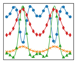
Figures 1 and 2 show the state of the four variables ( $Q_p^*$, $\langle c_p^{*\prime } \xi _p^{*\prime } \rangle$, $\langle \xi _p^{*\prime } \xi _p^{*\prime } \rangle$ and $E^*$) when $\max ( Q_p^* ) = \frac {1}{2}$. The first thing we notice is that both systems will tend to reach an equilibrium where all the variables reach a uniform constant state. We also observe that the charge profile differs significantly from those predicted by Kolehmainen et al. (Reference Kolehmainen, Ozel and Sundaresan2018b) and Montilla et al. (Reference Montilla, Ansart and Simonin2020). This is because, in their derivation, they neglected the effect of the charge variance in the modelling of the kinetic dispersion term. In our case, the charge variance effect leads to the production of charge–velocity covariance. Comparing the two studied cases, we remark a few differences between them. First of all, the magnitude of the charge covariance is much higher in the system with larger collision time. This is expected, as we know that the particle–particle collisions are a limiting factor in the kinetic dispersion effect, by limiting the mean free path of particles. As for the variance profile, we notice that there are two maximum values. These regions correspond to the zones where there is a maximum of the charge gradient and covariance. This can be explained by examining the variance transport equation (5.4), where we can see that one of the production terms is the product between the charge gradient and the charge–velocity covariance.

Figure 1. Time dependent profiles of the predicted variables using the full second-moment transport equation modelling approach at  $t^* \approx 48$: (a) dimensionless charge, (b) dimensionless electric field, (c) dimensionless charge–velocity covariance and (d) dimensionless charge variance for the test case with a dimensionless collision time $\tau _c^*=10^{-4}$.

Figure 2. Time dependent profiles of the predicted variables using the full second-moment transport equation modelling approach at  $t^* \approx 0.16$ for the test case with a dimensionless collision time $\tau _c^*=10^{-1}$: (a) dimensionless mean particle electric charge, (b) dimensionless electric field, (c) dimensionless particle charge–velocity covariance, (d) dimensionless particle charge variance.
We can also compare this modelling approach with the one proposed previously by Montilla et al. (Reference Montilla, Ansart and Simonin2020) that relies on a single transport equation for the mean electric charge and an algebraic gradient model for the charge–velocity covariance without any charge variance term. For the sake of brevity, we will only compare against the test case with the largest dimensionless collision time ( $\tau _c^* = 10^{-1}$), because it is in this configuration where the differences are more noticeable because we are further from the hypothesis needed to derive the algebraic gradient model. Figure 3, shows a comparison of variable profiles at the same dimensionless time. First, we observe that the maximum value of the mean electric charge is lower when using an algebraic model for the covariance. This is due to an overestimation of the kinetic transport term by neglecting the transient dynamic of the covariance, especially at the beginning. Secondly, we remark that the profile of the mean electric charge is different. The model proposed by Montilla et al. (Reference Montilla, Ansart and Simonin2020) predicts a trigonometric-like profile, while the full second-order transport equation model predicts a more complex profile because it solves the covariance dynamics and it takes into account the effect of the mean electrostatic force. Finally, this comparison also highlights that, although the algebraic gradient model might overestimate the charge–velocity covariance at the beginning, the opposite might be true later. In this case we observe that the gradient model underestimates the covariance, this is mainly because overestimating the kinetic transport reduced too quickly the mean charge gradient that produced the covariance but also because that simple algebraic model completely neglected any mean electrostatic force effect.

Figure 3. Comparison between the full second-moment transport equation model and the model proposed by Montilla et al. (Reference Montilla, Ansart and Simonin2020) for the test case with a dimensionless collision time  $\tau _c^{*} = 10^{-1}$. (a) Dimensionless mean particle electric charge. (b) Dimensionless electric field. (c) Dimensionless particle charge–velocity covariance. (d) Dimensionless particle charge variance.
Given the simplicity of these test cases, we can easily analyse the importance of the different phenomena taking place for the different variables. We can rearrange the transport equations and write them as  ${\partial \langle {\cdot } \rangle }/{\partial t} = \sum _i T_i$, where $T_i$ are the different production, destruction, dispersion, electrostatic, kinetic and collisional terms. Then, we can plot the profile for each of the $T_i$ to measure their weights in the configuration dynamics. This is done in figures 4 and 5, where we represent the profile for each contribution for the three transport equations. First of all, figures 4(a) and 5(a) confirm that the main charge transport mechanism in these cases is the kinetic transport due to the random motion of particles. However, the larger the collision time, the stronger the kinetic transport effects due to the larger particle mean free path.

Figure 4. Balance of the transport equations for the system with a lower collision time  $\tau _c^*=10^{-4}$. (a) Dimensionless mean particle electric charge. (b) Dimensionless particle charge–velocity covariance. (c) Dimensionless particle charge variance.

Figure 5. Balance of the transport equations for the system with a larger collision time  $\tau _c^*=10^{-1}$. (a) Dimensionless mean particle electric charge. (b) Dimensionless particle charge–velocity covariance. (c) Dimensionless particle charge variance.
For the covariance equation terms (figures 4b and 5b), the different terms are grouped together into different categories: production, destruction, dispersion and electrostatic force. Looking at these figures, the first thing we remark is that, in both cases, the main contributor to the covariance dynamics is the electrostatic force. The strength of this term is directly linked to the electric and kinetic energy ratio and the particle charge variance. Another important contribution comes from the destruction terms. There are two main mechanism that destroy the particle charge–velocity covariance: particle–particle collisions limiting the mean free path and modifying the particle electric charge at each collision, and the drag force that slows down the particle along its trajectory. The latter was neglected in our simulations ( $\tau _p^*=\infty$). Hence, the only destruction mechanism is due to the particle–particle collisions. And finally, in both cases, we observe a small production term. This production term is the generation of covariance due to the charge gradient. Although the two cases are very similar in the aspects mentioned above, there are important differences. First of all, we can see that the dispersion term obtained from the algebraic modelling of the third-order correlation is more noticeable in the system with larger collision time. The second noticeable difference is the temporal derivative term. In the smaller collision time case, the destruction and production terms are in equilibrium, making the transient term negligible. In other words, for small enough collision times, the charge–velocity covariance is in a quasi-steady state. This is due to the fact that, in these test cases, the covariance characteristic dissipation time is controlled by the collision time (because $\tau _p^*=\infty$ and $\tau _{\xi } \gg \tau _c^*$). Hence, a small collision time ensures a rapid relaxation towards a quasi-steady state characterized by an equilibrium between the production and dissipation terms of the transport equation (3.1).
Finally, the analysis of the variance terms (figures 4c and 5c) also reveals important information. First, we can note that both figures are very similar, and they only differ in the magnitude of the terms. In these examples, two contributions stand out: the production term related to the product between the charge gradient and the covariance (second term on the left-hand side of (5.4)), and the dispersion term coming for the algebraic model of the third-order correlation. In both cases, the modelling of the high-order correlation is an important term that should not be neglected.
These simple test cases allowed us to study in detail the different mechanisms present in the dynamics of a gas–solid flow with an electrostatic force. By analysing the individual contributions in the transport equations, we have shown that, under certain configurations, the transient term or the third-order moment can be neglected without losing any accuracy. On the other hand, we have also highlighted that systems with highly electrically charged particles require a correct modelling of the charge variance in order to predict the transport generated by the electrostatic force.
7. Reduced-order models
In this section, we would like to explore if we can reduce the complexity of the model, while accounting for as many physical phenomena as possible.
7.1. Full coupled algebraic model
The simplest approach could be to try to extend the algebraic model proposed by Montilla et al. (Reference Montilla, Ansart and Simonin2020) to take into account the electric charge variance. This will reduce the model to a single partial differential equation with two algebraic expressions for the charge–velocity covariance vector and the charge variance. In order to obtain this more general algebraic model, we can follow the methodology used to derive the previous algebraic model. First, we simplify the charge–velocity covariance and the charge variance equations neglecting the contributions of the Lagrangian derivative, the velocity gradient, the third-order moments and the dispersion terms. This reduces the covariance transport equation (3.1) and the variance transport equation (4.1) to the following system of algebraic equations:
 \begin{equation} \left\{\begin{array}{@{}l}
D_1 \langle c_{p,i}^{\prime} \xi_p^{\prime} \rangle +
D_{2,i} \langle \xi_p^{\prime} \xi_p^{\prime} \rangle =
D_{3,i} \\ F_{1,i} \langle c_{p,i}^{\prime} \xi_p^{\prime}
\rangle + F_2 \langle \xi_p^{\prime} \xi_p^{\prime} \rangle
= F_3 \end{array} \right.
\end{equation}
\begin{equation} \left\{\begin{array}{@{}l}
D_1 \langle c_{p,i}^{\prime} \xi_p^{\prime} \rangle +
D_{2,i} \langle \xi_p^{\prime} \xi_p^{\prime} \rangle =
D_{3,i} \\ F_{1,i} \langle c_{p,i}^{\prime} \xi_p^{\prime}
\rangle + F_2 \langle \xi_p^{\prime} \xi_p^{\prime} \rangle
= F_3 \end{array} \right.
\end{equation}
where
 $$\begin{gather} D_1 = \frac{1+e_c}{3}\frac{1}{\tau_c} + \frac{1}{\tau_p} + \frac{(3-e_c)}{5} \frac{1}{\tau_{\xi}} \end{gather}$$
 $$\begin{gather}D_{2,i} ={-}\frac{n_p}{m_p} E_i \end{gather}$$
 $$\begin{gather}D_{3,i} ={-}\left( 1 + \lambda_{2.2} e_c\frac{\sqrt{\varTheta_p}}{d_p} D_p \right)n_p\frac{\partial Q_p}{\partial x_i} + \lambda_{2.1} e_c \frac{\sqrt{\varTheta_p}}{d_p}\sigma_p E_i \end{gather}$$
 $$\begin{gather}F_{1,i} = 2n_p\frac{\partial Q_p}{\partial x_i} \end{gather}$$
 $$\begin{gather}F_{2} = n_p \left( \frac{1}{\tau_{\xi}} -\lambda_{3.1}(D_p)^2 \frac{\tau_c}{d_p^4} \right) \end{gather}$$
 $$\begin{gather}F_{3} = \lambda_{3.2}(\sigma_p)^2\frac{\tau_c}{n_p d_p^2} E_iE_i. \end{gather}$$
This system of equations can be solved to find an algebraic model coupling the particle charge–velocity covariance and the charge variance
 $$\begin{gather} \langle c_{p,i}^{\prime} \xi_p^{\prime} \rangle = \frac{D_{3,i}}{D_{1}} - \frac{D_{2,i}}{D_1}\langle \xi_p^{\prime} \xi_p^{\prime} \rangle, \end{gather}$$
 $$\begin{gather}\langle \xi_p^{\prime} \xi_p^{\prime} \rangle = \frac{F_3D_1 - F_{1,i}D_{3,i}}{D_1F_2 - D_{2,j}F_{1,j}}. \end{gather}$$
 Equations (7.8) and (7.9) give us a set of algebraic expressions that can be used to close the mean particle electric charge transport equation. With these expressions, we no longer have to solve a system of multiple partial differential equations (PDEs). We would also like to remark that this model reduces to the aforementioned simpler algebraic model of Montilla et al. (Reference Montilla, Ansart and Simonin2020) if  $\langle \xi _p^{\prime } \xi _p^{\prime } \rangle = 0$. So this model is indeed a more general algebraic model including the effects of the charge variance.
However, we would like to note that this algebraic closure law could produce non-physical results. In particular, the positive sign in (7.9) cannot be guaranteed. In addition to this, the denominator of this equation could also approach zero, leading to indeterminate variance values in some regions. A clear example of this can be shown if we look at the variance prediction for the initial condition of the two cases studied earlier (figure 6a,b). These figures show that this coupled algebraic model could lead to an unphysical prediction even for valid initial conditions. Given this behaviour, we cannot use this approach to simulate these two test cases. In our tests, we remarked that this problem is more prone to occur when the variance term is not negligible.

Figure 6. Initial variance profile predicted by the coupled algebraic model for the two cases studied; (a)  $\tau _c^*=10^{-4}$, (b) $\tau _c^*=10^{-1}$.
7.2. Semi-algebraic model
Another possible reduced-order model can be derived by only simplifying one of the second-order moment transport equations. Here, we choose to simplify the charge–velocity covariance transport equation to an algebraic expression. Therefore, the system is governed by the mean charge transport equation (2.24), the variance transport equation (4.1) and the algebraic simplification for the covariance (7.8). The reason behind this choice is that, as shown in the dimensionless analysis, the variance characteristic relaxation time will always be larger than the covariance characteristic relaxation time. Therefore, the quasi-steady state hypothesis can be reached first for the covariance but it is harder to satisfy for the variance.
We tested this approach for the same two configurations we have been studying in this paper. The first thing we would like to point out is that, unlike the previous model, this semi-algebraic model produced meaningful physical results at all times. Figures 7 and 8 show a comparison between this semi-algebraic model and the solution of the full second-order transport equation model. We observe that, in the smaller collision time configuration, the proposed semi-algebraic model matches perfectly the result obtained by solving the full model. However, for the larger collision time configuration, the semi-algebraic model fails to correctly reproduce the dynamics.

Figure 7. Comparison between the predictions of the full transport equation model and the semi-algebraic model in the test case with  $\tau _c^*=10^{-4}$. (a) Dimensionless mean particle electric charge. (b) Dimensionless electric field. (c) Dimensionless particle charge–velocity covariance. (d) Dimensionless particle charge variance.

Figure 8. Comparison between the predictions of the full transport equations model and the semi-algebraic model in the test case  $\tau _c^*=10^{-1}$. (a) Dimensionless mean particle electric charge. (b) Dimensionless electric field. (c) Dimensionless particle charge–velocity covariance. (d) Dimensionless particle charge variance.
In order to explain the success and failure of this model, we need to look at the hypotheses taken to reduce the covariance transport equation to an algebraic expression. The algebraic expression is obtained by assuming that the temporal derivative and any dispersion term can be neglected. Therefore, the semi-algebraic model should produce good results when these two assumptions hold simultaneously. This is exactly the case for the small collision time configuration. The term-by-term analysis of the covariance terms (figure 4b) showed that the transient and the kinetic dispersion terms are negligible compared with the production and destruction terms. In this case, the small collision time imposes also a very small relaxation characteristic time for the covariance, which ensures the quasi-steady state, corresponding to equilibrium between production and destruction terms. Also, the covariance dispersion coefficient is limited by the smallest of the particle collision time, the particle relaxation time and the variance destruction time. In our case, the very small particle collision time ensures a very weak covariance dispersion coefficient that could be neglected.
However, in the larger collision time configuration, the semi-algebraic model is not a suitable alternative. In this case, the assumptions mentioned above are no longer valid and therefore none of the terms in the equation can be neglected. The large collision time also means that the covariance characteristic destruction time is very large which means that no quasi-steady state can be reached. Also, the kinetic dispersion term is stronger as the collision times becomes larger. This is confirmed by looking at the term-by-term analysis of this case (figure 5b). We can clearly see that both the dispersion and temporal derivative terms are relevant to correctly characterize the dynamics of the covariance. In our example, we see that the semi-algebraic model has overestimated the mean charge transport. This is due to the overestimation of the kinetic transport imposed by the quasi-steady-state hypothesis.
Given these results, we wanted to determine the validity region in which the semi-algebraic model is a valid alternative to model the dynamics of a gas flow system with electrostatic charge. In order to do this, we performed several simulations varying the different dimensionless numbers to see the impact on the quality of the semi-algebraic model. According to our results, two of the most important parameters to determine the suitability of the semi-algebraic model are  $\tau _c^*$ and $Pe$. Using our simulations, we were able to distinguish the conditions in which the semi-algebraic model is a valid approach to model these kinds of systems, as shown by figure 9. We have also marked the two test cases we have studied in this article. As we can see, the boundary is a nonlinear curve. For high $Pe$ values we only need to ensure that the collision time is small enough to guarantee rapid relaxation towards the steady state and a weak kinetic dispersion for the charge covariance. However, as $Pe$ decreases, the electric charge transport due to collision increases. So the collision time has to be small enough to continue to ensure the quasi-steady-state hypothesis in the charge–velocity covariance transport equation.

Figure 9. Suitability regions of the semi-algebraic model as a function  $Pe$ and $\tau _c^*$. The two marked points correspond to the test cases studied in this work.
8. Conclusions
In this work, we have extended the Eulerian modelling of the mean electric charge transport equation. The simple algebraic gradient model for the electric charge kinetic flux term proposed in previous works was replaced with a more complete model using the full charge–velocity covariance transport equation. The charge variance term, which was neglected in the algebraic model, was closed using also the corresponding equation obtained in the frame of the kinetic theory of rapid granular flow. We have also proposed closure laws for the third-order charge and velocity correlations appearing in the covariance and variance transport equations.
This more complete approach was analysed in a one-dimensional periodic domain configuration. The simplicity of this test case allowed us to perform a dimensional analysis to obtain seven independent dimensionless numbers governing the system. In this work, we focused our attention on the kinetic regime of gas–solid flows, as it is in these configurations where the modelling of the particle charge–velocity covariance and particle variance is important. Our results showed that, in order to be in the kinetic regime, the product between the inverse of dimensionless dispersion coefficient and the dimensionless covariance relaxation time must be large.
We chose to study two different test cases in the kinetic regime, one with a low dimensionless particle collision time and one with a large particle collision time. But both under strong effects of the electrostatic forces. Our results showed that, when the electrostatic force is strong enough, the particle charge variance needs to be correctly modelled to capture the kinetic transport due to the mean electric field. We also showed that, when the particle collision time is small enough, the particle charge–velocity covariance is in a quasi-steady state, characterized by a local equilibrium between production and dissipation, and the third-order correlation effect is negligible. However, for large enough particle collision times, this quasi-steady state is not present, and the modelling of the high-order moments is important.
Because we were aware that adding and solving these additional transport equations may be too computationally expensive for practical applications, we also proposed and tested some possible simplifications. Our first attempt was to derive a coupled algebraic model that takes into account the electric charge variance. Although, mathematically feasible, the final result proved to be non-physical under some conditions, especially when the electrostatic force is strong. This means that this coupled algebraic model cannot be used when the variance term is dominant, which goes against the main objective of the model. Due to this important shortcoming, we proposed a different alternative in which the charge–velocity covariance retains the algebraic form including the variance term, however, the charge variance is obtained solving its transport equation. This intermediary model showed excellent agreement compared with the full model on the test case with a low particle collision time, but it completely failed on the test case with a larger particle collision time. This is because larger collision times imply a non-equilibrium particle charge–velocity covariance dynamics, which goes against one of the assumptions used to derive the algebraic model. Given these results, we also wanted to find under which conditions this semi-algebraic model could be suitable. In our study, we found that the two most important parameters to predict the suitability of this semi-algebraic approach are  $Pe$ and $\tau _c^*$. We performed several simulations varying these parameters, and we were able to determine under which conditions this reduced-order model can safely be used.
Finally, in order to derive the model presented in this work, a significant number of assumptions and hypotheses have been made and the lifting of these restrictions could be the subject of future studies. Some aspects should correspond to direct extensions of the proposed approach, such as the consideration of polydispersion or the effect of the short-range electrostatic particle–particle interaction on the collision dynamics. But others, according to our knowledge, seem to be more complex to take into account, such as the treatment of the polarization of the particles during the collisions or the modelling of the spatial and temporal fluctuations of the electric field due to the instantaneous distribution of the particles.
Acknowledgements
The authors would like to express their sincere appreciation to Professor M.W. Reeks for his many helpful and insightful comments that have significantly improved this paper.
Funding
This work was supported by the ANR–PAF project, grant ANR-16-CE06-0008 of the French National Agency of Research (ANR).
Declaration of interests
The authors report no conflict of interest.
Appendix A. Algebraic gradient closure model for the third-order moment $\langle \xi _p^{\prime } c_{p,i}^{\prime } c_{p,j}^{\prime } \rangle$

The transport equation of the particle charge–velocity covariance  $\langle \xi _p^{\prime } c_{p,i}^{\prime } \rangle$ depends on a higher-order statistical moment $\langle \xi _p^{\prime } c_{p,i}^{\prime } c_{p,j}^{\prime } \rangle$. In order to close the third-order statistical moment, we can use the same strategy employed to approximate the second-order statistical moments: an algebraic model. For this, we write the transport equation for this third-order moment using the general mean transport equation with $\phi = \xi _p^{\prime } c_{p,i}^{\prime } c_{p,j}^{\prime }$
 \begin{align} & n_{p}\frac{D\langle \xi_{p}^{\prime}c_{p,i}^{\prime}c_{p,j}^{\prime}\rangle }{Dt}+n_{p}S_{p,ijk}\frac{\partial Q_{p}}{\partial x_{k}}+n_{p}\langle \xi_{p}^{\prime}c_{p,k}^{\prime}\rangle \frac{\partial R_{p,ij}}{\partial x_{k}}+n_pR_{p,ik}\frac{\partial\langle \xi_{p}^{\prime}c_{p,j}^{\prime}\rangle }{\partial x_{k}}\nonumber\\ &\qquad + n_p R_{p,jk}\frac{\partial \langle \xi_{p}^{\prime}c_{p,i}^{\prime}\rangle }{\partial x_{k}}+n_{p}\frac{2}{\tau_{p}}\langle \xi_{p}^{\prime}c_{p,i}^{\prime}c_{p,j}^{\prime}\rangle -\frac{n_{p}}{m_{p}}\langle \xi_{p}^{\prime}c_{p,j}^{\prime}\xi_{p}^{\prime}\rangle E_{i}\nonumber\\ &\qquad -\frac{n_{p}}{m_{p}}\langle \xi_{p}^{\prime}c_{p,i}^{\prime}\xi_{p}^{\prime}\rangle E_{j} +n_{p}\langle c'_{p,k}c_{p,j}^{\prime}\xi_{p}^{\prime}\rangle \frac{\partial U_{p,i}}{\partial x_{k}}+n_{p}\langle c'_{p,k}c_{p,i}^{\prime}\xi_{p}^{\prime}\rangle \frac{\partial U_{p,j}}{\partial x_{k}} \nonumber\\ &\quad = \mathcal{C}(\xi_{p}c_{p,i}^{\prime}c_{p,j}^{\prime})-Q_{p}U_{p,i}\mathcal{C} (c_{p,j}) - Q_pU_{p,j}\mathcal{C}(c_{p,i})-\langle\xi_{p}^{\prime}c_{p,i}^{\prime}\rangle \mathcal{C}(c_{p,j})\nonumber\\ &\qquad -\langle \xi_{p}^{\prime}c_{p,j}^{\prime}\rangle \mathcal{C}(c_{p,i})-R_{p,ij}\mathcal{C}(\xi_{p}), \end{align}
with  $S_{p,ijk} = \langle c_{p,i}^{\prime } c_{p,j}^{\prime } c_{p,k}^{\prime } \rangle$.
Here, the equations of  $\langle \xi _p \rangle$, $\langle c_{p,i} \rangle$ $\langle \xi _p^{\prime } c_{p,i}^{\prime } \rangle$ and $\langle c_{p,i}^{\prime } c_{p,j}^{\prime } \rangle$ have been used to further simplify the final expression. We have also treated the force term in the same way as for the covariance equation: the undisturbed flow properties and the macroscopic electric field are assumed to be uncorrelated with the particles fluctuant electric charge.
In order to derive an algebraic model, we need to close the collision terms, in particular the term involving the third-order moment. To be able to derive an algebraic model we need a more general model to take into account the particle charge–velocity correlation in the collision integrals. We therefore propose an extension of the collision model proposed by Montilla et al. (Reference Montilla, Ansart and Simonin2020). In this work, we suppose that the conditional mean  $\langle \xi _{p_1} \mid \boldsymbol {c_{p_1}} \rangle$ can be written as
 \begin{equation} \langle \xi_{p} \mid \boldsymbol{c_{p}} \rangle = A + B_i c_{p,i}^{\prime} + C_{ij} c_{p,i}^{\prime}c_{p,j}^{\prime}. \end{equation}
 The tensors  $A$,
$A$,  $B_i$ and $C_{ij}$ are calculated so the first three statistical moments are satisfied
 $$\begin{gather} \int_{\mathbb{R}^3}\langle \xi_{p} \mid \boldsymbol{c_{p_1}} \rangle f\,{\rm d}\boldsymbol{c_p} = n_p \langle \xi_{p} \rangle, \end{gather}$$
 $$\begin{gather}\int_{\mathbb{R}^3} c_{p,i}^{\prime} \langle \xi_{p} \mid \boldsymbol{c_{p}} \rangle f\,{\rm d}\boldsymbol{c_p} = n_p \langle c_{p}^{\prime} \xi_{p} \rangle, \end{gather}$$
 $$\begin{gather}\int_{\mathbb{R}^3} c_{p,i}^{\prime} c_{p,j}^{\prime} \langle \xi_{p} \mid \boldsymbol{c_{p}} \rangle f\,{\rm d}\boldsymbol{c_p} = n_p \langle c_{p,i}^{\prime} c_{p,j}^{\prime} \xi_{p} \rangle. \end{gather}$$
 If we assume that the particle-velocity probability density function follows a Gaussian distribution, the fourth-order tensor  $\langle c^{\prime }_{p,i} c^{\prime }_{p,j}c^{\prime }_{p,k}c^{\prime }_{p,l} \rangle$ can be written as
 \begin{equation} \langle c^{\prime}_{p,i} c^{\prime}_{p,j}c^{\prime}_{p,k}c^{\prime}_{p,l} \rangle = R_{p,ij}R_{p,kl} + R_{p,ik}R_{p,jl} + R_{p,il}R_{p,jk}. \end{equation}
Assuming an isotropic kinetic stress tensor, we obtain
 \begin{equation} \langle c^{\prime}_{p,i} c^{\prime}_{p,j}c^{\prime}_{p,k}c^{\prime}_{p,l} \rangle = \varTheta_p^2\left( \delta_{ij}\delta_{kl} + \delta_{ik}\delta_{jl} + \delta_{il}\delta_{jk} \right). \end{equation}
 This allows us to deduce the expressions for the tensors  $A$,
$A$,  $B_i$ and $C_{ij}$
 $$\begin{gather} A = \langle \xi_p \rangle - \frac{1}{2\varTheta_p} \langle \xi_{p} c_{p,i}^{\prime} c_{p,j}^{\prime} \rangle, \end{gather}$$
 $$\begin{gather}B_i = \frac{1}{\varTheta_p}\langle c_{p,i}^{\prime} \xi_p \rangle, \end{gather}$$
 $$\begin{gather}C_{ij} = \frac{1}{\varTheta_p^2}\langle c_{p,i}^{\prime} c_{p,j}^{\prime} \xi_p \rangle. \end{gather}$$
This nonlinear model reduces exactly to the already published linear model if we assume  $\langle \xi _p c_{p,i}^{\prime }c_{p,j}^{\prime } \rangle = 0$.
With this model, we can now compute the right-hand side of (A1). For this term, we will assume a isotropic kinetic stress tensor. We also neglect any velocity and granular temperature gradient, as well as any cross-product term between  $Q_p$, $E_i$, $\langle c_{p,i}^{\prime } \xi _p^{\prime } \rangle$, $\langle \xi _p^{\prime } \rangle$, $\langle \xi _p^{\prime } \xi _p^{\prime } c_{p,i} \rangle$
 \begin{align} &\text{Right-hand side}\nonumber\\ &\quad={-}\frac{n_p}{\tau_{c}}[\lambda_{2.4}(1+e_{c})-\lambda_{2.5}(1+e_{c})^{2}]\langle \xi_{p}^{\prime}c_{p,i}^{\prime}c_{p,j}^{\prime}\rangle\nonumber\\ &\qquad +\frac{n_p}{\tau_{c}}[-\lambda_{2.7}(1+e_{c})+\lambda_{2.8}(1+e_{c})^{2}]\langle \xi_{p}^{\prime}c_{p,m}^{\prime}c_{p,m}^{\prime}\rangle\delta_{ij} -\lambda_{2.6}\frac{n_p}{\tau_{\xi}}\langle \xi_{p}^{\prime}c_{p,i}^{\prime}c_{p,j}^{\prime}\rangle\nonumber\\ & \qquad-n_pd_p\varTheta_{p}^{{1}/{2}}\left(1+e_{c}\right)\frac{1}{\tau_{\xi}}\left[\lambda_{2.9}\frac{\partial\langle \xi_{p}^{\prime}c_{p,i}^{\prime}\rangle }{\partial x_{j}}+ \lambda_{2.9}\frac{\partial\langle \xi_{p}^{\prime}c_{p,j}^{\prime}\rangle }{\partial x_{i}} +\lambda_{2.10}\frac{\partial\langle \xi_{p}^{\prime}c_{p,n}^{\prime}\rangle }{\partial x_{n}}\delta_{ij}\right]\nonumber\\ & \qquad-\lambda_{2.11}n_pd_p\varTheta_{p}^{{1}/{2}}\left(1+e_{c}\right)^{2}\frac{1}{\tau_{\xi}}\left[\frac{\partial\langle \xi_{p}^{\prime}c_{p,n}^{\prime}\rangle }{\partial x_{n}}\delta_{ij}+\frac{\partial\langle \xi_{p}^{\prime}c_{p,i}^{\prime}\rangle }{\partial x_{j}} + \frac{\partial\langle \xi_{p}^{\prime}c_{p,j}^{\prime}\rangle }{\partial x_{i}}\right] \end{align}
with  $\lambda _{2.4} \approx 6.667$, $\lambda _{2.5} \approx 1.387$, $\lambda _{2.6} \approx 3.201$, $\lambda _{2.7} \approx 0.2667$, $\lambda _{2.8} \approx 0.2607$, $\lambda _{2.9} \approx 10.68$, $\lambda _{2.10} \approx 208.2$ and $\lambda _{2.11} \approx 0.2048$.
Equations (A1) and (A11) give the form of a simple governing equation for the third-order moment  $\langle \xi _p^{\prime } c_{p,i}^{\prime } c_{p,j}^{\prime } \rangle$. To extract an algebraic closure model, we simplify the left-hand side of (A1) by neglecting the contribution of the Lagrangian time derivative, the velocity and kinetic stress gradient and the third-order tensors $S_{p,ijk}$ and $\langle \xi _p^{\prime } \xi _p^{\prime } c_{p,i}^{\prime } \rangle$. With these assumptions, we can write (A1) as
 \begin{equation} K_1 \langle \xi_p^{\prime} c_{p,i}^{\prime} c_{p,j}^{\prime} \rangle + K_2 \langle \xi_p^{\prime} c_{p,m}^{\prime} c_{p,m}^{\prime} \rangle \delta_{ij} = D_{ij}, \end{equation}
with
 $$\begin{gather} K_1 = n_p\left[\frac{1}{\tau_c}( \lambda_{2.4}\left(1+e_{c}\right)-\lambda_{2.5}\left(1+e_{c}\right)^{2} ) + \frac{1}{\tau_p} + \lambda_{2.6}\frac{1}{\tau_{\xi}} \right], \end{gather}$$
 $$\begin{gather}K_2 ={-}\frac{n_p}{\tau_{c}}[-\lambda_{2.7}\left(1+e_{c}\right)+\lambda_{2.8}\left(1+e_{c}\right)^{2}] , \end{gather}$$
 \begin{align} D_{ij} &= n_pR_{p,jk} \frac{\partial \langle \xi_p c_{p,i}^{\prime} \rangle}{\partial x_k} + n_pR_{p,ik} \frac{\partial \langle \xi_p c_{p,j}^{\prime} \rangle}{\partial x_k} \nonumber\\ &\quad -n_pd_p\varTheta_{p}^{{1}/{2}}\left(1+e_{c}\right)\frac{1}{\tau_{\xi}}\left[\lambda_{2.9}\frac{\partial\langle \xi_{p}^{\prime}c_{p,i}^{\prime}\rangle }{\partial x_{j}}+ \lambda_{2.9}\frac{\partial\langle \xi_{p}^{\prime}c_{p,j}^{\prime}\rangle }{\partial x_{i}} + \lambda_{2.10}\frac{\partial\langle \xi_{p}^{\prime}c_{p,n}^{\prime}\rangle }{\partial x_{n}}\delta_{ij}\right]\nonumber\\ &\quad -\lambda_{2.11}n_pd_p\varTheta_{p}^{{1}/{2}}\left(1+e_{c}\right)^{2}\frac{1}{\tau_{\xi}}\left[\frac{\partial\langle \xi_{p}^{\prime}c_{p,n}^{\prime}\rangle }{\partial x_{n}}\delta_{ij}+\frac{\partial\langle \xi_{p}^{\prime}c_{p,i}^{\prime}\rangle }{\partial x_{j}} + \frac{\partial\langle \xi_{p}^{\prime}c_{p,j}^{\prime}\rangle }{\partial x_{i}} \right]. \end{align}
In a three-dimensional flow, (A12) can be solved for the third-order moment
 \begin{equation} \langle \xi_p^{\prime} c_{p,i}^{\prime} c_{p,j}^{\prime} \rangle = \frac{1}{K_1}D_{ij} - \frac{K_2}{K_1\left( K_1 + 3K_2 \right)}D_{mm}\delta_{ij}. \end{equation}
Appendix B. Algebraic gradient closure model for the third-order moment $\langle \xi _p^{\prime } \xi _p^{\prime } c_{p,i}^{\prime } \rangle$

Similarly to the particle charge–velocity covariance equation, the particle charge variance equation is function of a higher statistical moment  $\langle \xi _p^{\prime } \xi _{p}^{\prime } c_{p,i}^\prime \rangle$. To close this term, we follow the same methodology used to close the previous third-order moment. First, we write the full transport equation for this third-order moment using the general mean transport equation with $\phi =\xi _p^{\prime } \xi _p^{\prime } c_{p,i}^{\prime }$
 \begin{align} &n_{p}\frac{D\langle \xi_{p}^{\prime}\xi_{p}^{\prime}c_{p,i}^{\prime}\rangle }{Dt}+ 2n_{p}\langle \xi_{p}^{\prime}c_{p,i}^{\prime}c_{p,j}^{\prime}\rangle \frac{\partial Q_{p}}{\partial x_{j}}+n_{p}\langle c_{p,i}^{\prime}c_{p,j}^{\prime}\rangle \frac{\partial\langle \xi_{p}^{\prime}\xi_{p}^{\prime}\rangle }{\partial x_{j}}\nonumber\\ &\quad + 2n_{p}\langle \xi_{p}^{\prime}c_{p,j}^{\prime}\rangle \frac{\partial\langle \xi_{p}^{\prime}c_{p,i}^{\prime}\rangle }{\partial x_{j}}+\frac{n_{p}}{\tau_{p}}\langle \xi_{p}^{\prime}\xi_{p}^{\prime}c_{p,i}^{\prime}\rangle -\frac{n_{p}}{m_{p}}\langle \xi_{p}^{\prime}\xi_{p}^{\prime}\xi_{p}^{\prime}\rangle E_{i}\nonumber\\ &\quad +n_{p}\langle \xi_{p}^{\prime}\xi_{p}^{\prime}c_{p,j}^{\prime}\rangle \frac{\partial U_{p,i}}{\partial x_{j}} =\mathcal{C}(\xi_{p}^{\prime}\xi_{p}^{\prime}c_{p,i}^{\prime})-2\langle \xi_{p}^{\prime}c_{p,i}^{\prime}\rangle \mathcal{C}(\xi_{p}^{\prime})-\langle \xi_{p}^{\prime}\xi_{p}^{\prime}\rangle \mathcal{C}(c_{p,i}^{\prime}). \end{align}
Here, the force term was treated using the same methodology as in Appendix A.
Assuming an isotropic kinetic stress tensor and neglecting the particle mean velocity gradient and the granular temperature gradient, we obtain a simplified form for the right-hand side of (B1)
 \begin{align} &\mathcal{C}(\xi_{p}^{\prime}\xi_{p}^{\prime}c_{p,i}^{\prime})-2\langle \xi_{p}^{\prime}c_{p,i}^{\prime}\rangle \mathcal{C}(\xi_{p}^{\prime})-\langle \xi_{p}^{\prime}\xi_{p}^{\prime}\rangle \mathcal{C}(c_{p,i}^{\prime})\nonumber\\ &\quad ={-}\left[\frac{1}{3}(1+e_{c})\frac{1}{\tau_{c}}+( 2.806 - 1.017 \gamma \varTheta_p^{{2}/{5}}) \frac{1}{\tau_{\xi}} \right]n_{p}\langle \xi_{p}^{\prime}\xi_{p}^{\prime}c_{p,i}^{\prime}\rangle. \end{align}
 Similarly to the previous algebraic gradient model, we simplify the left-hand side of (B1) by neglecting the contribution of the Lagrangian time derivative, the velocity and kinetic stress gradient and the third-order tensors  $S_{p,ijk}$ and $\langle \xi _p^{\prime } c_{p,i}^{\prime } c_{p,j}^{\prime } \rangle$. We will also drop any nonlinear term involving $\langle \xi _p^{\prime } c_{p,i} \rangle$, $E_i$ or $Q_p$. These assumptions lead us to the following closure model for the third-order moment:
 \begin{equation} n_p \langle \xi_p^{\prime} \xi_p^{\prime} c_{p,i}^{\prime} \rangle = \frac{n_pR_{p,ij}}{\dfrac{1}{3}\left(1+e_{c}\right)\dfrac{1}{\tau_{c}} + \dfrac{1}{\tau_p} +(\lambda_{3.4} - \lambda_{3.5} \gamma \varTheta_p^{{2}/{5}}) \dfrac{1}{\tau_{\xi}} } \dfrac{\partial \langle \xi_p^{\prime} \xi_p^{\prime} \rangle}{\partial x_j} \end{equation}
with  $\lambda _{3.4} \approx 2.806$ and $\lambda _{3.5} \approx 1.017$.


