


1. Introduction
The rheology of a suspension of rigid particles in a Newtonian fluid has been well studied analytically (Einstein Reference Einstein1906; Batchelor & Green Reference Batchelor and Green1972; Brenner Reference Brenner1974; Dabade, Marath & Subramanian Reference Dabade, Marath and Subramanian2016), experimentally (Krieger Reference Krieger1972; de Kruif et al. Reference de Kruif, van Iersel, Vrij and Russel1985; Van der Werff & De Kruif Reference Van der Werff and De Kruif1989; Zarraga, Hill & Leighton Reference Zarraga, Hill and Leighton2000; Singh & Nott Reference Singh and Nott2003; Snook et al. Reference Snook, Davidson, Butler, Pouliquen and Guazzelli2014) and computationally (Bossis & Brady Reference Bossis and Brady1984; Ladd Reference Ladd1994; Singh & Nott Reference Singh and Nott2000; Gallier et al. Reference Gallier, Lemaire, Lobry and Peters2014; Butler & Snook Reference Butler and Snook2018). However, there are many examples of suspensions in nature and in industrial settings wherein the suspended particles are deformable, in the form of fluid droplets, vesicles, capsules or elastic particles; blood is an example of such a suspension, comprising cells of a range of deformability. In these cases, an imposed shear flow causes the particles to change shape, and determination of their evolving shapes is central to determining the rheology of the suspension. Even for suspensions that are dilute enough that interaction between particles may be ignored, the rheology is non-Newtonian due to the deformation of an isolated particle caused by the imposed flow. The shape dynamics of fluid droplets and its influence on the suspension rheology has been studied for several decades (Oldroyd Reference Oldroyd1953; Cox Reference Cox1969; Stone Reference Stone1994; Wetzel & Tucker Reference Wetzel and Tucker2001; Jackson & Tucker Reference Jackson and Tucker2003; Minale Reference Minale2010; Mwasame, Wagner & Beris Reference Mwasame, Wagner and Beris2017). In recent years, more attention has been devoted to the dynamics of vesicles and capsules (Kraus et al. Reference Kraus, Wintz, Seifert and Lipowsky1996; Rioual, Biben & Misbah Reference Rioual, Biben and Misbah2004; Kantsler & Steinberg Reference Kantsler and Steinberg2006; Misbah Reference Misbah2006; Danker et al. Reference Danker, Biben, Podgorski, Verdier and Misbah2007; Danker & Misbah Reference Danker and Misbah2007; Noguchi & Gompper Reference Noguchi and Gompper2007; Zhao & Shaqfeh Reference Zhao and Shaqfeh2011; Guedda, Benlahsen & Misbah Reference Guedda, Benlahsen and Misbah2014).
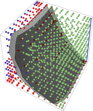
Most of the studies on deformable elastic and viscoelastic particles are restricted to the small deformation regime, wherein the constitutive relation for the elastic stress is effectively linear (Fröhlich & Sack Reference Fröhlich and Sack1946; Cerf Reference Cerf1952; Goddard & Miller Reference Goddard and Miller1967). The first systematic investigation of finite and large deformation of viscoelastic particles suspended in a Newtonian fluid was presented by Roscoe (Reference Roscoe1967), who used the neo-Hookean and Mooney–Rivlin constitutive models for the elastic stress. Roscoe's study was confined to the steady conformation (shape and orientation) of particles that are initially spherical (i.e. before shear is commenced). With the assumption that the particle undergoes homogeneous deformation in an ambient linear flow (where the undisturbed strain rate  $\dot {\gamma }$ is a constant), Roscoe deduced that the particle traverses a sequence of ellipsoidal shapes with changing aspect ratios and orientation, as shown in figure 1, until a steady conformation is reached. At steady state, material points within the ellipsoidal particle execute a ‘tank-treading’ motion. Making use of Jeffery's result for the fluid velocity field around a rigid ellipsoid (Jeffery Reference Jeffery1922) and imposing continuity of traction at the particle surface, the particle shape and its contribution to the suspension stress were determined in terms of the elastic capillary number $G \equiv \mu \dot {\gamma }/\eta$, where $\mu$ and $\eta$ are the viscosity of the suspending fluid and the elastic shear modulus of the particle, respectively. The existence of the tank-treading steady state was numerically verified in two (circles; see Gao & Hu Reference Gao and Hu2009) and three dimensions (spheres; see Gao, Hu & Castañeda Reference Gao, Hu and Castañeda2011), thereby validating the assumption of homogeneous deformation by Roscoe (Reference Roscoe1967).

Figure 1. Soft elastic particle deforming through a series of ellipsoidal shapes due to applied shear. The intensity of colour indicates the magnitude of the stress along the major axis of the ellipsoid.
Gao et al. (Reference Gao, Hu and Castañeda2011) developed a semi-analytical method for determining the shape dynamics of elastic ellipsoids obeying the neo-Hookean constitutive relation, but restricted attention to initially spherical particles. The analysis was extended to prolate spheroids whose symmetry axis is in the plane of shear by Gao, Hu & Castaneda (Reference Gao, Hu and Castaneda2012). Using the stress polarization technique introduced by Eshelby (Reference Eshelby1957, Reference Eshelby1959) for an elastic inclusion in an elastic matrix, the authors related the time derivative of the stress to the strain rate and vorticity fields inside the elastic particle through fourth-order shape tensors. The method yields a set of coupled nonlinear ordinary differential equations for the aspect ratios, orientation and the (three) stress components, which was solved numerically to obtain the transient response. An important aspect of this study is that, in addition to the tumbling motion expected in the near-rigid (small  $G$) limit, the authors showed the presence of a novel trembling motion that had earlier been observed in vesicles (Kantsler & Steinberg Reference Kantsler and Steinberg2006; Misbah Reference Misbah2006; Zhao & Shaqfeh Reference Zhao and Shaqfeh2011) and further, determined the tumbling–trembling phase diagram in the $G$–
$G$– $\omega _{0}$ plane.
A key step in the method of Gao et al. (Reference Gao, Hu and Castañeda2011, Reference Gao, Hu and Castaneda2012) is to obtain a relation between the time derivative of the stress and the strain rate by taking the upper convected time derivative of the neo-Hookean constitutive relation. However, for more general constitutive relations, such as Mooney–Rivlin, the time derivative of the stress cannot be related to the strain rate alone – the strain too will appear in the relation, thereby precluding the use of this method. It is therefore more appropriate to take the conventional approach in elasticity, where the stress is related to the strain or deformation. We show that the deformation at each instant of time can be obtained by recognizing that Roscoe's method (Roscoe Reference Roscoe1967) for determining the stress in the fluid can be extended to dynamically evolving states; enforcing continuity of the traction at the particle surface gives relations for the strain rate and vorticity within the particle, which in turn are related to the time evolution of the shape and orientation. Importantly, this method provides physical insight into the nature of the shape dynamics. For instance, we see that the rate of change of orientation of the particle has two contributions, one due to vorticity-induced rotation and the other to stretching of the particle along a direction different from its principal axes. For simple shear flow, these two components are of opposite sign for a range of orientations, and their relative magnitudes decide whether a tumbling or trembling dynamics occurs; a steady state can be attained only when the two contributions are precisely balanced. Although we restrict our attention to the in-plane dynamics for the case of simple shear flow, wherein two principal axes of the spheroid are in the plane of shear, our approach is general enough that the dynamics resulting from arbitrary initial orientations can be obtained; the latter will be considered in a subsequent paper.
The following caveat must be made with regard to the solutions we obtain by assuming the particle to be ellipsoidal at all times (equivalently, assuming the stress and deformation in the particle to be always uniform). Eshelby (Reference Eshelby1957, Reference Eshelby1959) showed that the ellipsoidal shape is the only solution for a linear elastic inclusion in a linear elastic medium; this was later extended to Newtonian drops in a Newtonian fluid by Wetzel & Tucker (Reference Wetzel and Tucker2001). In both cases, the constitutive relations for the dispersed and continuous phases are linear. When the inclusion is a nonlinear elastic solid, it is not known a priori that the shape will be ellipsoidal. The only assertion we can make is that the assumption of ellipsoidal shape yields a solution – however, this need not be the only solution. Nevertheless, the numerical validation of Gao & Hu (Reference Gao and Hu2009); Gao et al. (Reference Gao, Hu and Castañeda2011) is an indication that the solutions are physically relevant ones.
The paper is organized as follows. In § 2, we present our method for determining the shape dynamics of an isolated ellipsoidal particle suspended in a Newtonian fluid whose undisturbed flow is simple shear. The governing equations are then specialized for the in-plane dynamics of elastic and viscoelastic particles. In § 3, we solve the governing equations, where we first show that the results of Gao et al. (Reference Gao, Hu and Castaneda2012) for elastic spheres and prolate spheroids are recovered by our method (Appendix C). We then obtain the in-plane dynamics of elastic particles that are initially oblate spheroids or triaxial ellipsoids and construct the respective phase diagrams of dynamical states in the  $G$–aspect ratio space. The effect of viscoelasticity on the shape dynamics is then discussed. We conclude in § 4 with a summary of our main findings, the inferences drawn from them, and the potential applications of our study.
2. Mathematical formulation
In this section, we derive the equations that govern the dynamics of the particle shape, orientation and stress. Our interest is in the dynamics of a dilute suspension of small particles of nominal size  $\ell _p$ dispersed in viscous Newtonian liquids of density $\rho$ and viscosity $\mu$, with the suspension subjected to a uniform macroscopic strain rate. The bulk properties of such a suspension may be determined from the analysis of a single particle suspended in the fluid subjected to an undisturbed uniform strain rate of magnitude $\dot \gamma$. We further restrict attention to the flow regime where the Reynolds number $Re \equiv \rho \dot {\gamma }^2 \ell _p^2/\mu$ is negligibly small. Therefore, we may ignore the effects of inertia and solve the quasistatic equations of motion in the fluid and the elastic particle.
Roscoe (Reference Roscoe1967) considered the steady shape and orientation of elastic and viscoelastic particles whose stress-free shape is a sphere. When the undisturbed strain rate in the fluid is spatially uniform, he hypothesized that the particle would approach the steady state by traversing a series of ellipsoidal shapes wherein the strain rate in the particle is uniform at every instant. At steady state, every material point must be in continuous motion along a closed elliptical path, i.e. the deformed particle executes a ‘tank-treading’ motion. We wish to determine the transient and unsteady dynamics of initially stress-free ellipsoidal particles, for which Roscoe's analysis is not directly applicable. However, an aspect of Roscoe's analysis, namely the determination of the fluid stress for a given shape and orientation of the ellipsoid, may be easily extended for dynamical states. We describe this aspect of Roscoe's analysis in § 2.1 and its extension to dynamical states in § 2.2. By enforcing continuity of traction on the particle surface, we relate the strain rate and vorticity in the particle to the stress at a given instant of time in § 2.2, and from them obtain relations for the shape dynamics in § 2.3. We then obtain the stress in the particle in terms of the incremental change in shape from the previous time instant in § 2.4, thereby closing the problem. The method described in this section for determining the shape dynamics is applicable for arbitrary linear velocity fields  ${\boldsymbol {u}}^\infty$, but we consider only simple shear flow in this paper.
2.1. Stress in the fluid
Consider a neutrally buoyant deformable ellipsoidal particle suspended in an unbounded Newtonian fluid subjected to a uniform undisturbed velocity gradient  ${\boldsymbol{L}}^\infty \equiv {\boldsymbol {\nabla u^\infty }}$. In the fixed laboratory Cartesian coordinate frame (figure 2), the only non-zero component of ${\boldsymbol{L}}^\infty$ for simple shear is ${\mathsf{L}}^\infty _{12} = \dot \gamma$. We restrict attention to initial orientations where two principal axes of the ellipsoid are in the 1–2 plane; for spheroids one of them is the symmetry axis. From considerations of symmetry, these two principal axes will always remain in the 1–2 plane. However, our method is general and may also be used for the out-of-plane dynamics arising from the initial orientation not being in the 1–2 plane.

Figure 2. Schematic depicting the semi-axis lengths and orientations of the principal axes of a particle whose initial (stress free) shape is (a) an oblate spheroid and (b) prolate spheroid or triaxial ellipsoid. The axes labelled ( $1,2,x_3$) are the coordinate axes in the fixed laboratory reference frame, and ( $x_1,x_2,x_3$) are the principal axes of the particle. The aspect ratios of the particle are defined as $\omega _1 = \alpha _2/\alpha _1$, $\omega _2 = \alpha _3/\alpha _1$, where the $\alpha _i$ are the lengths of the principal semi-axes.
Hereafter, all the quantities of interest are quoted or reported in dimensionless form (unless specifically stated otherwise): the strain rate and vorticity are scaled by  $\dot \gamma$, time by $\dot \gamma ^{-1}$ and stress (in the fluid and particle) by $\mu \dot \gamma$. Let ${\boldsymbol{D}}^\infty$ and ${\boldsymbol{W}}^\infty$ denote the undisturbed strain rate and vorticity tensors, respectively. As argued by Roscoe (Reference Roscoe1967) (and validated numerically by Gao et al. Reference Gao, Hu and Castañeda2011), the strain rate $\boldsymbol{\mathsf{D}}$ and vorticity $\boldsymbol{\mathsf{W}}$ in the particle vary in time but are spatially uniform. To determine the velocity and stress fields in the fluid, we follow Roscoe (Reference Roscoe1967) by subtracting $\boldsymbol{\mathsf{D}}$ and $\boldsymbol{\mathsf{W}}$, respectively, from the strain rate and vorticity at every point in the domain. As a result, the strain and vorticity fields now correspond to a rigid, non-rotating ellipsoid in a fluid of undisturbed strain rate $\boldsymbol{\mathsf{D}}' \equiv {\boldsymbol{D}}^\infty - \boldsymbol{\mathsf{D}}$ and vorticity $\boldsymbol{\mathsf{W}}' \equiv {\boldsymbol{W}}^\infty - \boldsymbol{\mathsf{W}}$. It follows from the linearity of Stokes equations that the velocity and stress fields in the fluid due to the deformable particle may be obtained by adding to the respective fields obtained for the above rigid particle problem, the contributions from the uniform strain rate and vorticity $\boldsymbol{\mathsf{D}}$ and $\boldsymbol{\mathsf{W}}$. As a result, the stress field in the fluid is
 \begin{equation} {{\boldsymbol{\sigma}}} = {\boldsymbol{\mathsf{T}}}' + 2 \boldsymbol{\mathsf{D}}, \end{equation}
where  ${\boldsymbol{\mathsf{T}}}'$ is the stress field around a rigid, non-rotating ellipsoid in a fluid of undisturbed strain rate and vorticity $\boldsymbol{\mathsf{D}}'$ and $\boldsymbol{\mathsf{W}}'$, respectively. The expression for ${\boldsymbol{\mathsf{T}}}'$ was given by Jeffery (Reference Jeffery1922), who studied the motion of rigid ellipsoidal particles in a Newtonian fluid subjected to homogeneous linear flow. Jeffery's expression was written compactly (with some errors in transcription corrected) by Roscoe (Reference Roscoe1967) as ${\boldsymbol{\mathsf{T}}}' = -p' {\boldsymbol{\mathsf{I}}} + \boldsymbol{\mathsf{A}}'$, where $p'$ is an arbitrary hydrostatic pressure and $\boldsymbol{\mathsf{A}}'$ depends on the shape and orientation of the ellipsoid and linearly on $\boldsymbol{\mathsf{D}}'$. Note that $\boldsymbol{\mathsf{A}}'$ is not necessarily traceless. The arguments leading to (2.1) ensure continuity of velocity on the particle surface.
It is convenient to use a coordinate frame that is instantaneously aligned with the principal axes of the ellipsoid (see figure 2), in which the equation of the surface is
 \begin{equation} \frac{x_1^2}{\alpha_1^2} + \frac{x_2^2}{\alpha_2^2} + \frac{x_3^2}{\alpha_3^2} = 1, \end{equation}
where  $\alpha _i$ are the lengths of the three principal semi-axes. The axis labels are chosen based on the initial shape: for oblate spheroids, the $x_1$ axis is the in-plane principal axis of smaller length. For prolate spheroids and triaxial ellipsoids, the $x_1$ axis is the in-plane principal axis of larger length. Thus, the $x_1$ axis for spheroids in the stress-free state coincides with the symmetry axis. The aspect ratios are defined as $\omega _1 = \alpha _2/\alpha _1$ and $\omega _2 = \alpha _3/\alpha _1$.
In the particle coordinate frame, the undisturbed strain rate and vorticity may be expressed in terms of the Euler angles measuring the orientation of the principal axes relative to the axes of the fixed laboratory frame. For the in-plane dynamics in simple shear, only the Euler angle in the plane of shear varies with time (the other two being zero) and the undisturbed strain rate and vorticity are
 \begin{equation}
{\boldsymbol{D}}^\infty = \begin{bmatrix}
\frac{1}{2}\sin 2\theta & \frac{1}{2}\cos 2\theta & 0 \\
\frac{1}{2}\cos 2\theta & \frac{-1}{2}\sin 2\theta & 0 \\ 0
& 0 & 0 \end{bmatrix}, \quad
{\boldsymbol{W}}^\infty = \begin{bmatrix} 0 &
\frac{1}{2} & 0 \\ \frac{-1}{2} & 0 & 0 \\ 0 & 0 & 0
\end{bmatrix}, \end{equation}
\begin{equation}
{\boldsymbol{D}}^\infty = \begin{bmatrix}
\frac{1}{2}\sin 2\theta & \frac{1}{2}\cos 2\theta & 0 \\
\frac{1}{2}\cos 2\theta & \frac{-1}{2}\sin 2\theta & 0 \\ 0
& 0 & 0 \end{bmatrix}, \quad
{\boldsymbol{W}}^\infty = \begin{bmatrix} 0 &
\frac{1}{2} & 0 \\ \frac{-1}{2} & 0 & 0 \\ 0 & 0 & 0
\end{bmatrix}, \end{equation}
where  $\theta$ is the angle subtended by the $x_1$ axis with the flow direction in the anti-clockwise direction (figure 2).
2.2. Strain rate and vorticity in the particle
To proceed further, we enforce continuity of traction at the particle surface
 \begin{equation} {{\boldsymbol{\sigma}}}^p \boldsymbol{\cdot} {\boldsymbol{n}} = {{\boldsymbol{\sigma}}} \boldsymbol{\cdot} {\boldsymbol{n}}, \end{equation}
where  ${{\boldsymbol{\sigma} }}^p$ is the (spatially uniform) stress in the particle and ${\boldsymbol {n}}$ is a unit vector normal to the surface. As ${{\boldsymbol{\sigma} }}^p$ is uniform, it suffices to enforce continuity of traction at the intersection of the ellipsoidal surface with each principal axis. From (2.1) and (2.4), continuity of the normal component of the traction ${\boldsymbol {n}} \boldsymbol{\cdot} {{\boldsymbol{\sigma} }} \boldsymbol{\cdot} {\boldsymbol {n}}$ at the intersection with the $i$ axis gives
 \begin{equation} {\boldsymbol{\mathsf{\sigma}}}^p_{ii}={-}p' +\hat{{\mathsf{A}}}'_{ii} + 2 {\mathsf{D}}_{ii}, \end{equation}
where  $\hat {A}'_{ij}$ is the value of $A'_{ij}$ at $x_i = \alpha _i$, $x_k = 0$ ( $k \ne i$). The pressures $p'$ in the fluid and $p$ in the particle (see (2.18)) may be eliminated by taking differences between the normal traction at the intersections of the principal axes with the surface of the ellipsoid,
 $$\begin{gather} {\boldsymbol{\mathsf{\sigma}}}^p_{11}-{\boldsymbol{\mathsf{\sigma}}}^p_{22} = (\hat{{\mathsf{A}}}'_{11}-\hat{{\mathsf{A}}}'_{22})+2(D_{11}-D_{22}), \end{gather}$$
 $$\begin{gather}{\boldsymbol{\mathsf{\sigma}}}^p_{11}+{\boldsymbol{\mathsf{\sigma}}}^p_{22}-2{\boldsymbol{\mathsf{\sigma}}}^p_{33} = (\hat{{\mathsf{A}}}'_{11}+\hat{{\mathsf{A}}}'_{22}-2\hat{{\mathsf{A}}}'_{33})+6(D_{11}+D_{22}). \end{gather}$$
The expression for  $\hat {{\mathsf{A}}}'_{11}$ is (Roscoe Reference Roscoe1967)
 \begin{equation} \hat{{\mathsf{A}}}'_{11}=\frac{4}{3}\frac{2g''_{1}(D'_{11} - D_{11}) - g''_{2}(D'_{22} - D_{22}) - g''_{3}(D'_{33} - D_{33})}{g''_{1}g''_{2}+g''_{2}g''_{3}+g''_{3}g''_{1}}. \end{equation}
The expressions for  $\hat {{\mathsf{A}}}'_{22}$ and $\hat {{\mathsf{A}}}'_{33}$ are obtained by cyclic permutation of indices in (2.7). Here, $g''_i$ are functions of the semi-axis lengths $\alpha _i$ defined by Roscoe (Reference Roscoe1967); they are reproduced in Appendix A for the convenience of the reader. For the state of steady orientation and shape, the terms ${\mathsf{D}}_{ii}$ in (2.5)–(2.7) should be set to zero (see (2.16)); this was the state considered by Roscoe. As we wish to determine the transient and unsteady dynamics, we must retain these terms.
Substituting the expressions for  $\hat {{\mathsf{A}}}'_{ii}$ in (2.6) and rearranging the terms, we get
 \begin{align} {\boldsymbol{\mathsf{\sigma}}}^p_{11}-{\boldsymbol{\mathsf{\sigma}}}^p_{22} &= 5(\left(I_{12} + J_{12}\right)\left(D^{\infty}_{11}-D_{11}\right) \nonumber\\ &\quad + \left(I_{12} - J_{12}\right)\left(D^{\infty}_{22}-D_{22}\right)) + 2\left(D_{11}-D_{22}\right), \end{align}
 \begin{align} {\boldsymbol{\mathsf{\sigma}}}^p_{11}+{\boldsymbol{\mathsf{\sigma}}}^p_{22}-2{\boldsymbol{\mathsf{\sigma}}}^p_{33} &= 5(\left(I_{12} + J_{12}\right)\left(D^{\infty}_{11}-D_{11}\right) + \left(I_{12} - J_{12}\right)\left(D^{\infty}_{22}-D_{22}\right) \nonumber\\ &\quad + 2 \left(I_{23} - J_{23}\right)\left(\left(D^{\infty}_{11}-D_{11}\right)+\left(D^{\infty}_{22}-D_{22}\right)\right)) \nonumber\\&\quad + 6 \left(D_{11}-D_{22}\right), \end{align}
where,
 \begin{align} I_{12}&= \frac{2}{5}\frac{g''_{1}+g''_{2}}{g}, \quad J_{12}=\frac{2}{5}\frac{g''_{1}-g''_{2}}{g}, \end{align}
 \begin{align} I_{23}&=\frac{2}{5}\frac{g''_{2}+g''_{3}}{g}, \quad J_{23}=\frac{2}{5}\frac{g''_{2}-g''_{3}}{g}, \end{align}
and  $g=g''_{2}g''_{3}+g''_{3}g''_{1}+g''_{1}g''_{2}$. Explicit expressions for $D_{11}$ and $D_{22}$ are obtained by solving (2.8a,b) and are provided in Appendix B.
Continuity of the tangential component of the traction  ${\boldsymbol {t}} \boldsymbol{\cdot} {{\boldsymbol{\sigma} }} \boldsymbol{\cdot} {\boldsymbol {n}}$, where ${\boldsymbol {t}}$ is a unit tangent on the 1-axis, gives
 \begin{equation} {\boldsymbol{\mathsf{\sigma}}}^p_{12} = \hat{{\mathsf{A}}}'_{12}+2D_{12}, \end{equation}
where
 \begin{equation}
\hat{{\mathsf{A}}}'_{12}=\frac{8[g_1(D^{\infty}_{12}-D_{12})
+ \alpha_{2}^{2} g'_3 (W^{\infty}_{12}-W_{12})]}{2g'_3(\alpha_{1}^{2}
g_1+\alpha_{2}^{2} g_2)}.
\end{equation}
\begin{equation}
\hat{{\mathsf{A}}}'_{12}=\frac{8[g_1(D^{\infty}_{12}-D_{12})
+ \alpha_{2}^{2} g'_3 (W^{\infty}_{12}-W_{12})]}{2g'_3(\alpha_{1}^{2}
g_1+\alpha_{2}^{2} g_2)}.
\end{equation}
The factors  $g_i$ and $g'_i$ are functions of the semi-axis lengths $\alpha _i$ (Roscoe Reference Roscoe1967) and are defined in Appendix A. Similarly, $\hat {{\mathsf{A}}}'_{21}$ can be obtained by interchanging the indices 1 and 2 in (2.11). Symmetry of ${{\boldsymbol{\sigma} }}^p$ requires that $\hat {{\mathsf{A}}}'_{12}=\hat {{\mathsf{A}}}'_{21}$, which yields the relation
 \begin{equation} (g_1-g_2)(D^{\infty}_{12}-D_{12}) ={-}(\alpha_{1}^2 +\alpha_{2}^2)g'_3(W^{\infty}_{12}-W_{12}). \end{equation}
Noting that  $g_1-g_2 = (\alpha _{1}^{2} - \alpha _{2}^{2})g'_3$, (2.12) results in the following relation between the strain rate and the vorticity fields inside the particle:
 \begin{equation} (W^{\infty}_{12}-W_{12}) = \frac{(\alpha_{1}^2 - \alpha_{2}^2)}{(\alpha_{1}^2 + \alpha_{2}^2)}(D^{\infty}_{12}-D_{12}). \end{equation}
Substituting (2.13) into the expression for  $\hat {{\mathsf{A}}}'_{12}$ and subsequently into (2.10) yields the expression for the shear stress in the 1–2 plane
 \begin{equation} {\boldsymbol{\mathsf{\sigma}}}^p_{12}=\frac{8\left[g_1 + \alpha_{2}^{2} g'_3 \left(\dfrac{\alpha_{1}^2 - \alpha_{2}^2}{\alpha_{1}^2 + \alpha_{2}^2} \right) \right] (D^{\infty}_{12}-D_{12}) }{2g'_3(\alpha_{1}^{2}g_1 + \alpha_{2}^{2} g_2)} + 2 D_{12}. \end{equation}
Expressions for  ${\boldsymbol{\mathsf{\sigma}}} ^p_{23}$ and ${\boldsymbol{\mathsf{\sigma}}} ^p_{13}$ (needed only for the off-plane dynamics) may be obtained by cyclic permutation of indices in (2.14). Equations (2.13) and (2.14) provide the required relations for $D_{12}$ and $W_{12}$; the expressions are lengthy and given in Appendix B.
Thus, with knowledge of the particle stress  ${{\boldsymbol{\sigma} }}^p$, we can determine $\boldsymbol{\mathsf{D}}$ and $\boldsymbol{\mathsf{W}}$ in the particle. The determination of ${{\boldsymbol{\sigma} }}^p$ from the instantaneous orientation and shape of the particle, starting from the stress-free configuration at $t = 0$, is discussed in § 2.4.
2.3. Evolution of particle shape and orientation
The evolution of the shape and orientation can be obtained in terms of the strain rate and vorticity in the particle using the formulation of Wetzel & Tucker (Reference Wetzel and Tucker2001). In the coordinate system instantaneously aligned with the particle principal axes at time  $t$ (but not co-rotating with it), the surface of the ellipsoid satisfies the equation ${\boldsymbol{S}} {\boldsymbol {:}} {\boldsymbol {x x}} = 1$, where ${\boldsymbol{S}}$ is the diagonal shape tensor with components ${\mathsf{S}}_{ii}=1/\alpha _i^2$. Applying the material derivative to this equation and using the definition of the instantaneous velocity field inside the particle, ${\boldsymbol {v}}= {\boldsymbol{L}} \boldsymbol{\cdot} {\boldsymbol {x}}$, where ${\boldsymbol{L}}$ is the uniform velocity gradient in the particle, the following relation can be obtained:
 \begin{equation} \dfrac{{\mathrm d} {\boldsymbol{S}}}{{\mathrm d} t} + {\boldsymbol{L}}^{{\rm T}} \boldsymbol{\cdot} {\boldsymbol{S}}+{\boldsymbol{S}} \boldsymbol{\cdot} {\boldsymbol{L}} = 0. \end{equation}
Note that  ${\mathrm d}{\boldsymbol{S}}/{\mathrm d} t$ is not diagonal, as a result of particle rotation; it is obtained by replacing ${\boldsymbol{S}}$ by ${\boldsymbol{S}}' = {\boldsymbol{\mathsf{R}}}(\theta ) \boldsymbol{\cdot} {\boldsymbol{S}} \boldsymbol{\cdot} {\boldsymbol{\mathsf{R}}}^{{\rm T}}(\theta )$, where ${\boldsymbol{\mathsf{R}}}(\theta )$ is the rotation tensor corresponding to a rotation by angle $\theta$ in the 1–2 plane, taking the time derivative of ${\boldsymbol{S}}'$, and then setting $\theta$ to zero. Equation (2.15) is the only aspect of the analysis of Wetzel & Tucker (Reference Wetzel and Tucker2001) that we use. In particular, we eschew using their method of writing the deformation rate and vorticity in the particle in terms of fourth rank ‘concentration tensors’, and use instead the more direct method described in § 2.2.
Substituting  ${\boldsymbol{L}}=\boldsymbol{\mathsf{D}}+\boldsymbol{\mathsf{W}}$, the diagonal components of (2.15) give relations for the time evolution of the semi-axis lengths,
 \begin{equation} \frac{1}{\alpha_i}\frac{{\mathrm d} \alpha_i}{{\mathrm d} t} = {\mathsf{D}}_{ii}, \end{equation}
and the off-diagonal 1–2 component yields the evolution equation for the orientation
 \begin{equation} \frac{{\mathrm d} \theta}{{\mathrm d} t} = \frac{\alpha_1^2+\alpha_2^2}{\alpha_1^2-\alpha_2^2} \, D_{12} - W_{12}. \end{equation}
At steady state, (2.17) yields the linear relation between  $D_{12}$ and $W_{12}$ obtained by Roscoe (Reference Roscoe1967).
2.4. Stress in the particle
We model the particle as an incompressible neo-Hookean solid, satisfying the constitutive relation
 \begin{equation} {{\boldsymbol{\sigma}}}^p={-}p{\boldsymbol{\mathsf{I}}}+{\boldsymbol{\mathsf{\tau}}} ={-}p{\boldsymbol{\mathsf{I}}} + \eta \, ({\boldsymbol{\mathsf{B}}}-{\boldsymbol{\mathsf{I}}}), \end{equation}
where  $p$ is the pressure in the solid that varies so as to enforce incompressibility, ${\boldsymbol{\mathsf{B}}}$ is the configuration dependent finger tensor (or the left Cauchy–Green deformation tensor) and $\eta$ is the elastic modulus. The finger tensor is defined as ${\boldsymbol{\mathsf{B}}} = {\boldsymbol {F}} \boldsymbol{\cdot} {\boldsymbol {F}}^{{\rm T}}$, where ${\boldsymbol {F}}={\boldsymbol {{\partial x}/{\partial X}}}$ is the deformation gradient tensor relating the configuration at time $t$ to the stress-free initial configuration. Note that (2.18) gives the stress in dimensional form; when scaled by $\mu \dot \gamma$ (see § 2.1), the dimensionless extra stress is ${\boldsymbol{\mathsf{\tau}}} = ({1}/{G}) ({\boldsymbol{\mathsf{B}}}-{\boldsymbol{\mathsf{I}}})$, where $G \equiv \mu \dot \gamma /\eta$ is the elastic capillary number. Determination of the stress requires ${\boldsymbol {F}}$, which we determine below from the deformation history of the particle.
2.4.1. Particle deformation in a small time interval  $\delta t$

Consider a time  $t_i$ at which the shape ( $\alpha _1$, $\alpha _2$, $\alpha _3$) and orientation ( $\theta$) of the particle are known (figure 3a). We determine the deformation in the time interval $\delta t$ that is small enough that the stress in the particle can be assumed to remain constant. The particle undergoes an in-plane rotation through an angle $-\zeta$ due to vorticity (see figure 3b). It also undergoes deformation by in-plane stretches $\lambda _1$ and $\lambda _2$ ( $\lambda _1 > \lambda _2$) (ratios of deformed lengths to original lengths of a differential material element) oriented at angles $\varphi$ and $\varphi + {\rm \pi}/2$, respectively, to the $x_1$ axis of the particle (see figure 3c); incompressibility requires the particle to be stretched by $\lambda _3 = 1/(\lambda _1 \lambda _2)$ in the 3-direction. Due to the misalignment between the directions of stretch and the particle axes, the orientation further changes such that the extensional stretch axis ( $\lambda _1$ axis) subtends an angle $\psi$ with the $x_1$ axis (figure 3f). All angles are defined as positive in the anti-clockwise direction. Note that the angles of rotation $\zeta$ and $\psi - \varphi$, and the deviations of the stretches from unity $\lambda _1 - 1$ and $\lambda _2 - 1$ are all proportional to $\delta t$. As a result of the changes in orientation due to vorticity and stretch, the orientation $\theta '$ at $t_{i+1} = t_i + \delta t$ is
 \begin{equation} \theta' = \theta - \zeta + \varphi - \psi. \end{equation}
Figure 3. Sequence of steps involved in mapping a material point from time  $t_i$ to $t_{i+1}$. All angles are positive in the anti-clockwise direction. (a) Particle at initial orientation $\theta$. (b) In-plane rotation of the particle due to the (uniform) vorticity field in the particle by an angle $-\zeta$. After rotation, the extensional stretch axis ( $\lambda _1$ axis) subtends an angle $\varphi$ with the $x_1$ axis of the particle. (c) Stretching of the particle due to the (uniform) strain rate at an angle $\varphi$ from its principal axes. After stretching, the extensional stretch axis subtends an angle $\psi$ with the $x_1$ axis. (d,e) Virtual transformations to effect stretching: in (d) the particle is rotated by $-(\theta - \zeta + \varphi )$ so that the stretch axes are aligned with the laboratory axes; in (e) the particle undergoes stretches of $\lambda _1$, $\lambda _2$, $\lambda _3$ along the laboratory axes. After stretching, it is rotated by $(\theta - \zeta + \varphi )$. ( f) The conformation of the particle at $t_{i+1}$, after rotation and stretching.
Following the rotation and stretch, the mapping between positions of a material point, expressed in the laboratory reference frame, at times  $t_i$ and $t_{i+1}$ is
 \begin{equation} {\boldsymbol{y}}^{i+1} = {\boldsymbol{\mathsf{R}}}(\theta - \zeta + \varphi) \boldsymbol{\cdot} {\boldsymbol{\mathsf{T}}} \boldsymbol{\cdot} {\boldsymbol{\mathsf{R}}}(-\theta + \zeta - \varphi) \boldsymbol{\cdot} {\boldsymbol{\mathsf{R}}}(-\zeta) \boldsymbol{\cdot} {\boldsymbol{y}}^i, \end{equation}
where  ${\boldsymbol{\mathsf{T}}}$ is the diagonal stretch tensor with components $T_{ii} = \lambda _i$ and $\boldsymbol{\mathsf{R}}$ is the rotation tensor defined in § 2.3. The combination ${\boldsymbol{\mathsf{R}}}(\theta -\zeta + \varphi ) \boldsymbol{\cdot} {\boldsymbol{\mathsf{T}}} \boldsymbol{\cdot} {\boldsymbol{\mathsf{R}}}(-\theta + \zeta - \varphi )$ serves to transform the diagonal stretch tensor to the laboratory reference frame by accounting for the angle $\theta - \zeta + \varphi$ between the $\lambda _1$ axis of stretch and the flow direction (see figure 3c). Equation (2.20) may be written as
 \begin{equation} {\boldsymbol{y}}^{i+1} = {\boldsymbol{F}}^i \boldsymbol{\cdot} {\boldsymbol{y}}^i, \end{equation}
where  ${\boldsymbol {F}}^i$ is the deformation gradient tensor in the laboratory reference frame whose components have the values
 \begin{equation} \left. \begin{aligned} F^i_{11} & = \tfrac{1}{2}\{(\lambda_1+\lambda_2)\cos \zeta + (\lambda_1-\lambda_2)\cos (2\theta + 2\varphi - \zeta) \}, \\ F^i_{12} & = \tfrac{1}{2}\{(\lambda_1+\lambda_2)\sin \zeta + (\lambda_1-\lambda_2)\sin (2\theta + 2\varphi - \zeta) \}, \\ F^i_{21} & = \tfrac{1}{2}\{-(\lambda_1+\lambda_2)\sin \zeta + (\lambda_1-\lambda_2)\sin (2\theta + 2\varphi - \zeta) \}, \\ F^i_{22} & = \tfrac{1}{2}\{(\lambda_1+\lambda_2)\cos \zeta - (\lambda_1-\lambda_2)\cos (2\theta + 2\varphi - \zeta) \} \\ F^i_{13} & = F^i_{23} = F^i_{31} = F^i_{32} = 0; \quad F^i_{33} = \lambda_3. \end{aligned} \right\} \end{equation}
2.4.2. Relating the shape and orientation to the strain rate and vorticity
To evaluate  ${\boldsymbol {F}}^i$, we need the values of $\lambda _1$, $\lambda _2$, $\zeta$, $\varphi$ and $\psi$. From (2.17) and (2.19), the change in orientation due to vorticity and stretching, respectively, are given by
 $$\begin{gather} \zeta = W_{12} \, \delta t, \end{gather}$$
 $$\begin{gather}\varphi - \psi = \left(\frac{\alpha_1^2+\alpha_2^2}{\alpha_1^2-\alpha_2^2}\right) D_{12} \, \delta t, \end{gather}$$
with errors of O( $\delta t^2$). An additional equation comes from the condition that there is no shear along the principal stretch directions. It then follows from Mohr's circle for the strain rate that
 \begin{equation} \varphi = \frac{1}{2}\tan^{{-}1}\frac{2 D_{12}}{D_{11}-D_{22}}. \end{equation}
The relations (2.16) and (2.23) over the time step  $\delta t$ along with (2.24) give us updated lengths $\alpha _i$ of the semi-axes and the orientation $\theta '$, and the angles $\zeta$, $\varphi$ and $\psi$.
It now remains to calculate the stretches  $\lambda _1$ and $\lambda _2$ to obtain the deformation gradient tensor. For this, we consider the shape of the particle after it is stretched by the principal stretch tensor ${\boldsymbol{\mathsf{T}}}$. Consider the particle in figure 3(d), where it has been rotated so that the principal stretch axes align with the laboratory axes. The equation of the in-plane cross-section of the particle in laboratory coordinates before stretching is that of an ellipse at an angle $-\varphi$ to the 1-axis. Stretching transforms each point ( $y_1$, $y_2$, $y_3$) in the ellipsoid to ( $\lambda _1 y_1$, $\lambda _2 y_2$, $\lambda _3 y_3$), whence the equation of the cross-section after stretching is
 \begin{align} y_1^2\left(\frac{\cos^2\varphi}{\lambda_1^2\alpha_1^2} + \frac{\sin^2\varphi}{\lambda_1^2\alpha_2^2}\right) + y_2^2\left(\frac{\sin^2\varphi}{\lambda_2^2\alpha_1^2} + \frac{\cos^2\varphi}{\lambda_2^2\alpha_2^2}\right) - \frac{2 y_1 y_2}{\lambda_1\lambda_2}\left(\frac{1}{\alpha_1^2}-\frac{1}{\alpha_2^2}\right)\sin\varphi \cos\varphi = 1. \end{align}
The principal axis of the particle is now at an angle  $-\psi$ to the 1-axis (figure 3e), and its semi-axis lengths have changed to ( $\alpha _1'$, $\alpha _2'$, $\alpha _3'$), which are obtained by integrating (2.16) over the time interval $\delta t$. The equation of the cross-section can therefore be equivalently be written as
 \begin{align} y_1^2\left(\frac{\cos^2\psi}{\alpha_1'^2} + \frac{\sin^2\psi}{\alpha_2'^2}\right) + y_2^2\left(\frac{\sin^2\psi}{\alpha_1'^2} + \frac{\cos^2\psi}{\alpha_2'^2}\right)- 2y_1y_2\left(\frac{1}{\alpha_1'^2}-\frac{1}{\alpha_2'^2}\right)\sin\psi \cos\psi = 1. \end{align}
Comparing the coefficients of  $y_1^2$ and $y_2^2$ in (2.25) and (2.26), we get the required expressions for $\lambda _1$ and $\lambda _2$
 \begin{equation} \lambda_{1} =
\left(\dfrac{\dfrac{\cos^{2}\varphi}{\alpha_{1}^{2}} +
\dfrac{\sin^{2}\varphi}{\alpha_{2}^{2}}}{\dfrac{\cos^{2}\psi}{\alpha_{1}'^{2}}
+ \dfrac{\sin^{2}\psi}{\alpha_{2}'^{2}}}\right)^{{1}/{2}},
\quad \lambda_{2} =
\left(\dfrac{\dfrac{\sin^{2}\varphi}{\alpha_{1}^{2}} +
\dfrac{\cos^{2}\varphi}{\alpha_{2}^{2}}}{\dfrac{\sin^{2}\psi}{\alpha_{1}'^{2}}
+ \dfrac{\cos^{2}\psi}{\alpha_{2}'^{2}}}\right)^{{1}/{2}}.
\end{equation}
\begin{equation} \lambda_{1} =
\left(\dfrac{\dfrac{\cos^{2}\varphi}{\alpha_{1}^{2}} +
\dfrac{\sin^{2}\varphi}{\alpha_{2}^{2}}}{\dfrac{\cos^{2}\psi}{\alpha_{1}'^{2}}
+ \dfrac{\sin^{2}\psi}{\alpha_{2}'^{2}}}\right)^{{1}/{2}},
\quad \lambda_{2} =
\left(\dfrac{\dfrac{\sin^{2}\varphi}{\alpha_{1}^{2}} +
\dfrac{\cos^{2}\varphi}{\alpha_{2}^{2}}}{\dfrac{\sin^{2}\psi}{\alpha_{1}'^{2}}
+ \dfrac{\cos^{2}\psi}{\alpha_{2}'^{2}}}\right)^{{1}/{2}}.
\end{equation}
2.4.3. Particle stress in terms of the kinematic variables
The deformation gradient tensor  ${\boldsymbol {F}}^i$ in (2.22) relates positions of material points in the laboratory coordinate system between times $t_{i+1}$ and $t_i$. However, the constitutive relation for the elastic stress requires the deformation gradient ${\boldsymbol {F}}$ that relates the configuration at time $t_{i+1}$ to the stress-free configuration at $t_0 = 0$. This is simply the time-ordered contraction of ${\boldsymbol {F}}^i$ at all intermediate states
 \begin{equation} {\boldsymbol{F}} = {\boldsymbol{F}}^{i} \boldsymbol{\cdot} {\boldsymbol{F}}^{i-1} \ldots \,\boldsymbol{\cdot} {\boldsymbol{F}}^1 \boldsymbol{\cdot} {\boldsymbol{F}}^0. \end{equation}
The finger tensor in the fixed laboratory coordinate frame then is  ${\boldsymbol{\mathsf{B}}}_{lab} = {\boldsymbol {F}} \boldsymbol{\cdot} {\boldsymbol {F}}^{\rm T}$. As we require the particle stress in the coordinate system aligned with its principal axes (which subtend an angle of $\theta '$ with fixed laboratory coordinates),
 \begin{equation} {\boldsymbol{\mathsf{B}}} = {\boldsymbol{\mathsf{R}}}(-\theta') \boldsymbol{\cdot} {\boldsymbol{\mathsf{B}}}_{lab} \boldsymbol{\cdot} {\boldsymbol{\mathsf{R}}}(\theta') \end{equation}
is the appropriate finger tensor to determine the stress in (2.18).
2.5. Extension to viscoelastic particles
For a viscoelastic solid, the total stress is the sum of elastic and viscous contributions,  ${{\boldsymbol{\sigma} }}^p = {{\boldsymbol{\sigma} }}^e + {{\boldsymbol{\sigma} }}^v$. Determination of the elastic stress ${{\boldsymbol{\sigma} }}^e$ has already been outlined in § 2.4; the viscous contribution is ${{\boldsymbol{\sigma} }}^v = 2\kappa \boldsymbol{\mathsf{D}}$, where $\kappa$ is the viscosity ratio of the particle to the fluid. Balancing the normal and tangential components of the traction at the surface of the particle, and following the same procedure as in § 2.2 to eliminate the pressure, we get the following equations that extend (2.8) and (2.14) for a viscoelastic particle:
 \begin{align} {\boldsymbol{\mathsf{\sigma}}}^p_{11}-{\boldsymbol{\mathsf{\sigma}}}^p_{22} &= ({\boldsymbol{\mathsf{\sigma}}}^e_{11}-{\boldsymbol{\mathsf{\sigma}}}^e_{22}) + 2 \kappa \left(D_{11}-D_{22} \right) \nonumber\\ &= 5 \left(\left(I_{12} + J_{12}\right)\left(D^{\infty}_{11}-D_{11}\right) + \left(I_{12} - J_{12}\right)\left(D^{\infty}_{22}-D_{22}\right)\right) \nonumber\\ &\quad + 2 \left(D_{11}-D_{22}\right), \end{align}
 \begin{align} {\boldsymbol{\mathsf{\sigma}}}^p_{11}+{\boldsymbol{\mathsf{\sigma}}}^p_{22}-2{\boldsymbol{\mathsf{\sigma}}}^p_{33} &= ({\boldsymbol{\mathsf{\sigma}}}^e_{11} +{\boldsymbol{\mathsf{\sigma}}}^e_{22}-2{\boldsymbol{\mathsf{\sigma}}}^e_{33})+ 6 \kappa \left(D_{11}-D_{22}\right) \nonumber\\ &= 5(\left(I_{12} + J_{12}\right)\left(D^{\infty}_{11}-D_{11}\right) + \left(I_{12} - J_{12}\right)\left(D^{\infty}_{22}-D_{22}\right) \nonumber\\ &\quad + 2 \left(I_{23} - J_{23}\right)\left(\left(D^{\infty}_{11}-D_{11}\right)+\left(D^{\infty}_{22}-D_{22}\right)\right)) \nonumber\\ &\quad + 6 \left(D_{11}-D_{22}\right), \end{align}
 \begin{align}{\boldsymbol{\mathsf{\sigma}}}^p_{12} &= {\boldsymbol{\mathsf{\sigma}}}^e_{12} + 2 \kappa D_{12} \nonumber\\ &=\frac{8\left[g_1+\alpha_{2}^{2} g'_3 \left(\dfrac{\alpha_{1}^2 - \alpha_{2}^2}{\alpha_{1}^2 + \alpha_{2}^2}\right)\right](D^{\infty}_{12}-D_{12}) }{2~g'_3(\alpha_{1}^{2} g_1 + \alpha_{2}^{2} g_2)} + 2 D_{12} . \end{align}
Again, cyclic permutation of indices in  ${\boldsymbol{\mathsf{\sigma}}} ^p_{12}$ provides the expressions for ${\boldsymbol{\mathsf{\sigma}}} ^p_{23}$ and ${\boldsymbol{\mathsf{\sigma}}} ^p_{13}$. The components of the strain rate and vorticity fields in the viscoelastic particle can be obtained by solving (2.30) and are given in § B.2 of Appendix B.
2.6. Calculation of rheological properties
The bulk stress in the suspension is  $\langle {{{\boldsymbol{\sigma} }}}\rangle =\phi \langle {{\boldsymbol{\sigma} }}\rangle ^p +(1-\phi )\langle {{{\boldsymbol{\sigma} }}}\rangle ^f$, where $\phi$ is the particle volume fraction and the angle brackets represent volume averages. Similarly, the bulk strain rate of the suspension can be expressed in terms of the respective averages in the two phases, $\langle {\boldsymbol{\mathsf{D}}}\rangle =\phi \langle {\boldsymbol{\mathsf{D}}}\rangle ^p +(1-\phi )\langle {\boldsymbol{\mathsf{D}}}\rangle ^f$. Therefore, the suspension stress is
 \begin{equation}
\langle{{\boldsymbol{\mathsf{\sigma}}}}\rangle
={-}\langle{p}\rangle{\boldsymbol{\mathsf{I}}}+2\langle{\boldsymbol{\mathsf{D}}}\rangle+\phi
(\langle{{\boldsymbol{\mathsf{\tau}}}}\rangle^p-2\langle{\boldsymbol{\mathsf{D}}}\rangle^p).
\end{equation}
\begin{equation}
\langle{{\boldsymbol{\mathsf{\sigma}}}}\rangle
={-}\langle{p}\rangle{\boldsymbol{\mathsf{I}}}+2\langle{\boldsymbol{\mathsf{D}}}\rangle+\phi
(\langle{{\boldsymbol{\mathsf{\tau}}}}\rangle^p-2\langle{\boldsymbol{\mathsf{D}}}\rangle^p).
\end{equation}
Note that the bulk strain rate and vorticity are identical to the externally imposed flow quantities, i.e.  $\langle {\boldsymbol{\mathsf{D}}}\rangle =\boldsymbol{\mathsf{D}}^{\infty}$ and $\langle {\boldsymbol{\mathsf{W}}}\rangle =\boldsymbol{\mathsf{W}}^{\infty}$.
We consider the suspension to be composed of ellipsoids of identical size but different orientations in the initial (stress-free) state. As the suspension is dilute enough that particles do not interact, the undisturbed flow experienced by each particle is the imposed linear flow, for which the strain rate and stress within each particle at each instant of time are uniform. As a result,  $\langle {\boldsymbol{\mathsf{\tau}}}^{p} \rangle$ and $\langle \boldsymbol{\mathsf{D}}^{p} \rangle$ represent averages over the orientation of a single particle. We find that the long-time orientation dynamics for initial ellipsoidal particles is identical, to within a phase lag, regardless of the initial orientation; the phase lag is a residual signature of the short transient associated with the stress-free initial orientation. Therefore, the long-time average for ellipsoids over all initial orientations is identical to the average over a time period of tumbling or trembling; for initially spherical particles it is trivially the steady state.
The rheological properties of interest then are the intrinsic shear viscosity
 \begin{equation} [\mu]_s = \frac{\dfrac{\langle{{\boldsymbol{\mathsf{\sigma}}}}\rangle_{12}}{2{D}^{\infty}_{12}}-1}{\phi} = \langle \tau \rangle^{p}_{12} - 2 \langle D \rangle^p_{12}, \end{equation}
and the intrinsic normal stress differences in simple shear flow
 $$\begin{gather} N_{1} = \frac{\langle {\boldsymbol{\mathsf{\sigma}}} \rangle_{11}-\langle {\boldsymbol{\mathsf{\sigma}}} \rangle_{22}}{\phi} = ( \langle \tau \rangle^{p}_{11} - \langle \tau \rangle^{p}_{22}) - 2(\langle D \rangle^p_{11} - \langle D \rangle^p_{22}), \end{gather}$$
 $$\begin{gather}N_{2} = \frac{\langle{{\boldsymbol{\mathsf{\sigma}}}}\rangle_{22}-\langle{{\boldsymbol{\mathsf{\sigma}}}}\rangle_{33}}{\phi} = ( \langle \tau \rangle^{p}_{22} - \langle \tau \rangle^{p}_{33})-2(\langle D \rangle^p_{22} - \langle D \rangle^p_{33}). \end{gather}$$
3. Results and discussion
3.1. Dynamics of an elastic particle in simple shear flow
We study the shape dynamics of neutrally buoyant elastic particles whose initial (stress-free) shape is a sphere, a spheroid and, more generally, a triaxial ellipsoid, suspended in an unbounded Newtonian fluid subjected to simple shear. As mentioned in § 1, the shape dynamics of an initial sphere and prolate spheroid were reported earlier by Gao et al. (Reference Gao, Hu and Castañeda2011, Reference Gao, Hu and Castaneda2012). We validate our solution method by a comparison with their results; the comparison is provided in Appendix C, where it is shown that the two sets of results are identical. Thus, the primary new results reported here concern the in-plane dynamics of oblate spheroids and triaxial ellipsoids.
3.1.1. Dynamics of oblate spheroids and triaxial ellipsoids
As in the case of prolate spheroids (Gao et al. Reference Gao, Hu and Castaneda2012), oblate spheroids and triaxial ellipsoids too exhibit trembling and tumbling dynamics. We first discuss the shape dynamics of oblate spheroids. For a given initial aspect ratio  $\omega _{1,0} = \omega _{2,0} = \omega _0$, the particle deforms to resemble a thin disk for part of its tumbling/trembling cycle as the elastic capillary number $G$ increases. Since $G$ may be thought of as the inverse of the dimensionless stiffness, increasing $G$ implies increasing deformability. The transition from tumbling to trembling occurs at a critical value of $G$ that depends on $\omega _0$. Figures 4 and 5 show the results for two values of $G$ for $\omega _0=2.5$ on either side of the tumbling–trembling transition for an initial orientation of $\theta _0={\rm \pi} /2$ (i.e. the symmetry axis pointing in the velocity gradient direction). It is evident from figure 4(b) that the particle tumbles for $G=0.4$ and trembles for $G=0.5$.

Figure 4. Dynamics of an initially oblate spheroid exhibiting trembling and tumbling dynamics at  $\omega _0 = 2.5$. (a) In-plane and out-of-plane aspect ratios. (b) Orientation of the $x_1$ axis. The stress polarization results were obtained using the method of Gao et al. (Reference Gao, Hu and Castañeda2011).

Figure 5. (a,b) The time variation of the direction of stretch ( $\varphi$) for the two cases shown in figure 4, namely $G=0.4$ (a) and $G=0.5$ (b). The particle orientation from figure 4(b) is superposed. (c,d) The contributions to the change in orientation due to the vorticity ( $-\zeta$) and stretch ( $\varphi -\psi$), and the net change ( $\varphi -\psi -\zeta$) during each time step corresponding to panels (a,b). Refer to figure 3 for the definitions of the angles $\zeta$, $\phi$ and $\varphi$. The time step $\delta t$ is not constant, as it has to be adaptively changed to accurately compute sharp changes.
Figure 5(a,b) shows the variations with time of the orientation  $\theta$ and the angle $\varphi$ between the $x_1$ axis and tensile stretch axis. Recall from § 2.1 that the $x_1$ axis (which characterizes the orientation $\theta$) for an oblate spheroid is the in-plane principal axis of smaller length. For the stiffer particle ( $G=0.4$), $\varphi$ changes sign twice during a revolution (figure 5a), implying tumbling motion. The transition may be understood by considering the contributions to rotation from stretching and vorticity in every time step $\delta t$, shown in figure 5(c). We see that, although the orientation change due to stretching $\varphi -\psi$ is positive for part of each cycle, it is smaller in magnitude than the orientation change due to vorticity $-\zeta$; the net change in orientation $(\varphi - \psi ) - \zeta$ is therefore always negative, resulting in tumbling. For the softer particle ( $G=0.5$), $\varphi$ is always negative (figure 5b), implying that the $x_1$ axis lies between the flow direction and the direction of extensional stretch ( $\lambda _1$); the orientation change due to stretch is therefore always positive (figure 5d); it is also larger in magnitude that the orientation change due to vorticity. As a result, the particle trembles – the orientation oscillates about an angle that depends on $G$ and $\omega _0$. The sharp peaks in figure 5(c,d) correspond to instances when the in-plane aspect ratio ( $\omega _1$) is close to unity (figure 4a), about which there is rapid variation in $\varphi$ (figure 5a,b). The results presented in figures 4 and 5 are for an initial orientation wherein the $x_1$ axis is aligned with the gradient direction. Any other initial orientation in the plane of shear simply leads to the same dynamics at large time, apart from a short initial transient. Thus, the only signature of the initial orientation is a phase difference in the universal long-time dynamics.
For very stiff particles, such as  $G=0.01$, the orientation of the principal stretch axis exhibits the same qualitative dynamics as that in figure 5(a) for $G=0.4$. The transition from tumbling to trembling (for a fixed $\omega _0$) occurs with increasing $G$ due to the particle deforming into an increasingly anisotropic shape that causes it to spend enough time in orientations where the longer in-plane axis is close to the flow direction and the rate of rotation is the lowest, allowing the deformed particle to ‘spring back’. It is relevant to contrast the dynamics of elastic and rigid particles ( $G = 0$). As there is no stretch dynamics for the latter, they only tumble. Further, a key difference is that while the stress within the elastic particle remains uniform in the limit $G \to 0$, there is no requirement for the stress to be uniform at $G = 0$; indeed the stress in the latter case is indeterminate. However, we show below that the orientation dynamics of very stiff particles is virtually identical to a rigid one, implying that the stress indeterminacy is not of relevance to the dynamics.
We now come to the shape dynamics of triaxial ellipsoids. Recall from § 2.1 that the  $x_1$ axis in this case is the larger in-plane principal axis in the initial state. Figure 6 displays results for two ellipsoids of different initial aspect ratios with $G=0.2$, one exhibiting tumbling dynamics and the other trembling. As the stiffness is reduced, there is always a tumbling to trembling transition, no matter what the initial aspect ratios are, which we discuss below. An interesting aspect of elastic triaxial ellipsoids is that the orientation dynamics depends on the initial out-of-plane aspect ratio $\omega _{2,0}$; this is in contrast to rigid ellipsoids, where the dynamics is independent of $\omega _{2}$, as shown by Jeffery (Reference Jeffery1922). This difference between rigid and elastic ellipsoids is shown in figure 7; while the orientation dynamics for rigid ellipsoids of different out-of-plane aspect ratios is identical (figure 7a), there is a slow down of the tumbling dynamics for elastic particles with decreasing $\omega _{2,0}$, for small $G$, and a transition from tumbling to trembling with decreasing $\omega _{2,0}$ at the highest $G$ (figure 7b–d).

Figure 6. Dynamics of an initially ellipsoidal elastic particle in the trembling and tumbling regimes at  $G=0.2$. (a) In-plane and out-of-plane aspect ratios. (b) Orientation of the major axis.

Figure 7. Effect of out-of-plane aspect ratio on the dynamics of an initially ellipsoidal elastic particle with  $\omega _{1,0}=0.4$. (a) Perfectly rigid particle ( $G=0$). (b) Slightly soft particle with $G=0.01$. (c) Softer particle with $G=0.1$. (d) Soft particle with $G=0.4$.
3.1.2. Phase diagrams of dynamical states for spheroids and triaxial ellipsoids
As already discussed, for a particle that is initially an oblate spheroid of aspect ratio  $\omega _0$, the transition from tumbling to trembling occurs at a critical value of $G$. Thus, the tumbling–trembling transition can be shown in a $G$–
$G$– $\omega _0$ plot, as in the case of prolate spheroids (Gao et al. Reference Gao, Hu and Castaneda2012). Figure 8 shows the combined phase diagram for prolate and oblate spheroids. We know from Roscoe (Reference Roscoe1967) that an initially spherical particle ( $\omega _0=1$) reaches a steady shape and orientation, regardless of $G$; this state is represented by the blue vertical line. As the shape deviates from $\omega _0=1$ on either side, the particle exhibits a tumbling dynamics for small $G$ and trembling above a critical value of $G$, which increases as $\omega _0$ progressively deviates from unity on either side. Thus, extreme-aspect-ratio spheroids (slender rods or thin disks) transition to the trembling regime at a large shear rate for a given stiffness. The phase boundary separating the trembling and tumbling regimes is identified at a $(G,\omega _0)$ where the dynamics includes an instant of time when the cross-section in the plane of shear is circular ( $\omega _1 = 1$). The principal axes are interchanged at this instant, resulting in a jump in $\theta$ by $\pm {\rm \pi}/2$; the marginal trajectory on the phase boundary may therefore be regarded as a trembling or tumbling trajectory. Although the trembling–tumbling phase boundaries appear to be symmetric about the $\omega _0=1$ axis (suggesting an $\omega _0 \rightarrow 1/\omega _0$ equivalence), they are not (see inset of figure 8). This is a departure from the phase diagram for two-dimensional elliptical particles (infinitely long cylinders of elliptical cross-section), where the equations governing the shape dynamics are invariant under the transformation $\omega _0 \rightarrow 1/\omega _0$ (Gao et al. Reference Gao, Hu and Castaneda2012); indeed, the transformation in the two-dimensional case corresponds trivially to a rotation of the ellipse by ${\rm \pi} /2$.

Figure 8. Phase diagram of spheroids in simple shear flow. The types of dynamics exhibited are denoted by the labels SS for steady state, TR for trembling and TU for tumbling.
For a triaxial ellipsoid in simple shear flow, the phase boundary for the tumbling–trembling transition is a two-dimensional surface in ( $\omega _{1,0},\omega _{2,0}, G$) space. As accurate resolution of the phase boundary in the three-dimensional parameter space is computationally prohibitive, we only determine, for discrete values of $G$ and $\omega _{2,0}$, the upper and lower bounds of $\omega _{1,0}$ for tumbling and trembling that deviate from the true phase boundary by at most 0.05. They are represented by the light and dark grey surfaces in figure 9(a). Thus, for a given set of ( $G,\omega _{2,0}$), the lower (light grey) surface represents the lower bound of $\omega _{1,0}$ at which the particle trembles, and the upper (dark grey) surface represents the upper bound of $\omega _{1,0}$ at which it tumbles. Figure 9(b–d) shows sections of the phase diagram at fixed values of $G$,
$G$,  $\omega _{1,0}$ and $\omega _{2,0}$, respectively, so that features of the transition may be seen in greater detail. The vertical edges of the graph in figure 9(a) represent the following initial configurations of the particle: a sphere ( $\omega _{1,0}=\omega _{2,0}=1$), a circular disk whose normal is in the vorticity direction ( $\omega _{1,0}=1,\; \omega _{2,0}=0$), an infinitely slender rod ( $\omega _{1,0}=\omega _{2,0}=0$) in the plane of shear, and a circular disk with its normal in the plane of shear ( $\omega _{1,0}=0$ and $\omega _{2,0}=1$), respectively. The vertical planes represent the following initial configurations: the $\omega _{1,0}=1,\; \omega _{2,0} < 1$ plane represents an oblate spheroid whose symmetry axis is aligned in the vorticity direction, the $\omega _{1,0}=0,\; \omega _{2,0}<1$ plane represents an elliptical disk whose normal is in the plane of shear, the $\omega _{2,0}=1, \omega _{1,0} < 1$ plane represents an oblate spheroid whose symmetry axis is in the plane of shear, and the $\omega _{2,0} = 0,\; \omega _{1,0} < 1$ plane represents an elliptical disk whose normal is along the vorticity axis. Thus, the $\omega _{2,0}=1,\; \omega _{1,0} < 1$ plane contains the in-plane dynamics of oblate spheroids, and corresponds to the right half of figure 8. Finally, the diagonal vertical plane $\omega _{2,0} = \omega _{1,0}$ represents a prolate spheroid whose symmetry axis is in the plane of shear, and corresponds to the left half of figure 8. We see from figure 9(a) that thin elliptical disks in the plane of shear ( $\omega _{2,0} \rightarrow 0$) and oblate spheroids whose normal is in the plane of shear ( $\omega _{2,0} \rightarrow 1$) exhibit a tumbling–trembling transition as $G$ is increased, but thin elliptical disks with normal in the plane of shear ( $\omega _{1,0} \rightarrow 0$) exhibit either a tumbling or flow-aligning dynamics (see below) for the range of $G$ we have studied. An interesting point to note from figure 9(b,c) is that the tumbling–trembling transition is not significantly influenced by the out-of-plane aspect ratio $\omega _{2,0}$ beyond $0.5$; indeed, we find the threshold curve at $\omega _{2,0} = 1$ to be quite close to that for $\omega _{2,0} \rightarrow \infty$, which corresponds to elliptical cylinders aligned with the vorticity direction, examined by Gao et al. (Reference Gao, Hu and Castaneda2012).

Figure 9. Tumbling–trembling phase diagram of a triaxial ellipsoid in simple shear flow. (a) The filled red and green circles represent tumbling (TU) and trembling (TR) dynamical states, respectively. The filled blue circles represent flow-aligning states wherein the long axis of the particle asymptotically approaches the flow axis. The light and dark grey surfaces represent the upper and lower bounds in  $\omega _{1,0}$ for tumbling dynamics and trembling dynamics, respectively; the true phase boundary lies between them. (b–d) Sections of the phase diagram at (b) $G=0.5$, (c) $\omega _{1,0}=0.5$ and (d) $\omega _{2,0}=0.5$.
Below the lower (light grey) surface in figure 9(a), there are some points represented by the blue circles that denote states where the long axis of the particle does not cross the flow axis. The shape dynamics corresponding to one such point is shown in figure 10, where it is clear that the lengths of the in-plane semi-axes vary as  $\alpha _1 \sim t$, $\alpha _2 \sim 1/t$ in the limit $t \to \infty$, and the orientation $\theta$ decays to zero as $1/t$. The continuous stretching of the particle along its major axis slows down its rotation, leading to an asymptotic flow-aligning behaviour. For any $G > 0$, there is an interval of small $\omega _{1,0}$ for which the particle extends indefinitely in time and asymptotically aligns with the flow axis. We have not attempted to compute accurately the boundary between such flow-aligning states and the tumbling states, due to the long computation time required. While the flow-aligning state may be physically unrealistic – real elastic particles will undergo plastic deformation beyond a critical stress and eventually rupture – it still is an interesting feature, as it is likely to be present in any continuum elastic model that allows arbitrarily large deformation, and indicates the parameter regime for which particles are likely to rupture. We note that an indefinitely stretching flow-aligning state has also been predicted for an initially spherical liquid drop in a Newtonian fluid subjected to shear above a critical capillary number $\textit {Ca} \equiv \mu \dot {\gamma }\ell _p/{\boldsymbol{\mathsf{\sigma}}}$ ( ${\boldsymbol{\mathsf{\sigma}}}$ being the interfacial tension) by Wetzel & Tucker (Reference Wetzel and Tucker2001). Such an elongated drop will ultimately break up (Barthes-Biesel & Acrivos Reference Barthes-Biesel and Acrivos1973). There will, however, be differences in the mechanism of breakup between drops and elastic particles, as the Stokes equations governing motion in the former remain valid until breakup, while the neo-Hookean constitutive relation will cease to be valid beyond the point of plastic yield. Further discussion on the similarity and differences in the dynamics of drops, capsules and elastic particles is given in § 4.

Figure 10. Trajectory of an initial triaxial ellipsoid that asymptotically aligns with the flow direction. The parameter values are  $G = 1.0$, $\omega _{1,0} = 0.01$, $\omega _{2,0} = 0.05$. Time variation of (a) the orientation and (b) lengths of the principal semi-axes $\alpha _i$.
The rheological responses of dilute suspensions of initially oblate spheroids of aspect ratio  $\omega _{0}=2$ and triaxial ellipsoids of aspect ratios $\omega _{1,0}=0.7$, $\omega _{2,0}=0.8$ are shown in figure 11. As mentioned in § 2.6, the rheological properties were obtained by averaging over a cycle of the long-time oscillatory response, which is equivalent to averaging over different initial orientations. As $G$ may be thought of as a dimensionless shear rate, it is apparent from figure 11(a,c) that the suspension is shear thinning. The reason for this is straightforward to understand: with increasing $G$, the particle tends to extend and align towards the flow direction, thereby offering less resistance to deformation. The intrinsic shear viscosity $[\mu ]_s$ becomes negative for sufficiently large $G$ (which for the cases considered is $\sim 1$), as found by Gao et al. (Reference Gao, Hu and Castañeda2011, Reference Gao, Hu and Castaneda2012) for initially spherical and prolate spheroidal particles. This is a result of the extra dissipation in the fluid due to the presence of particles becoming small enough to be more than compensated by the lack of dissipation within the particles. An analogous change in sign of the intrinsic viscosity as a function of the capillary number Ca is known for magmas containing highly deformable bubbles (Manga & Loewenberg Reference Manga and Loewenberg2001). Figure 11(b,d) shows that the first and second normal stress differences are positive and negative, respectively; as $N_1/G$ and $N_2/G$ are proportional to the corresponding normal stress coefficients, the figure shows mild shear thinning of these coefficients too. A positive $N_1$ arises from the greater alignment of the longest axis, which is under tension, with the flow direction; a negative $N_2$ arises from the shortest axis, that is under compression, beginning to align with the gradient direction. The overall response is similar to that of a dilute suspension of rigid spheroids (Brenner Reference Brenner1974).

Figure 11. Rheological response of a dilute non-interacting suspension of elastic particles as a function of  $G$. The top row shows the (a) intrinsic viscosity and (b) normal stress differences for initial oblate spheroids of aspect ratio $\omega _{0}=2$. The bottom row shows the same quantities for initial ellipsoids of aspect ratios $\omega _{1,0}=0.7$, $\omega _{2,0}=0.8$.
Our analysis and results consider the particle to be in an initial stress-free state before shear is commenced. We briefly comment on what the dynamics might be if the particle were to have a residual stress in the initial state. The simplest case is when the initial state corresponds to one of the uniformly stressed configurations accessed in the dynamics across any of the steady tank-treading, trembling, tumbling or flow-aligning regimes described above: the dynamics of such an ellipsoid would correspond to that particular configuration, with the only difference being the absence of an initial transient. However, it is unlikely that the dynamics over the entire range of  $\omega _{1,0}$, $\omega _{2,0}$ and $G$ covers uniformly stressed ellipsoids of all possible orientations: for example, we do not see a sufficiently slender ellipsoid (that exhibits flow-aligning behaviour in the absence of an initial residual stress) having a finite stress in the compressional quadrant of the simple shear flow arising from a stress-free initial configuration. We may nevertheless make the following plausible speculation: we know that an ellipsoid with a uniform residual stress must relax, in the absence of an imposed shear, to a stress-free state through a sequence of ellipsoidal configurations; this suggests a close relation between the dynamics of such an ellipsoid and the (hypothetical) stress-free ellipsoid that it would relax to. It is then tempting to conclude that these two initial ellipsoidal configurations would converge to the same long-time dynamics, with differences restricted to an initial transient that is similar to initially stress-free configurations with differing orientations converging to the same long-time dynamics (see the discussion in § 2.6). If this were the case, the analysis in the manuscript subsumes the long-time dynamics of initially uniformly stressed ellipsoids. The long-time shape-cum-orientation dynamics of an ellipsoid with a non-uniform residual stress field in the initial state is beyond the scope of the present analysis. However, if the amplitude of the non-uniformity is small, then the shape dynamics would be accessible to a perturbative approach. As this weakly non-uniform residual stress would drive an approach to a marginally non-ellipsoidal stress-free state in the absence of an imposed shear, the analysis of such an initial state is likely to be equivalent to a stability analysis of initially ellipsoidal stress-free configurations to small-amplitude shape perturbations.
3.2. Effect of particle viscoelasticity
We now discuss the dynamics of viscoelastic particles in simple shear flow. The shape dynamics of initial spheres and spheroids, and the resulting dilute suspension rheology, are now influenced by  $G$ and $\kappa$, the ratio of the viscosity of the particle to that of the suspending fluid. As already discussed, an initially spherical elastic particle ( $\kappa =0$) attains a steady ellipsoidal shape with its longest axis orientated between the extensional and flow directions. For non-zero $\kappa$, an initial spherical particle exhibits a damped oscillatory approach to the eventual steady state, with the amplitude of the oscillations increasing with $\kappa$ to begin with (compare $\kappa = 0$ and $10$ in figure 12). However, in the limit $\kappa \rightarrow \infty$, the dynamics must approach that of a rigid sphere. This implies that the amplitude of shape oscillations must eventually decrease with increasing $\kappa$ (compare $\kappa = 10$ and $50$ in figure 12). Further, since a rigid sphere rotates with a uniform angular velocity (equalling half the ambient vorticity), the orientation dynamics must transition to a tumbling behaviour for sufficiently large $\kappa$, with $\theta$ continuously decreasing with time (not shown). In figure 12(d), the intrinsic shear viscosity increases with $\kappa$ until it reaches $2.5$, the Einstein coefficient for the limit $\kappa \rightarrow \infty$. On the other hand, the magnitudes of the first and second normal stress differences decrease with increasing $\kappa$ (figure 12e, f); they understandably tend to zero in the limit $\kappa \rightarrow \infty$, as in a dilute suspension non-interacting rigid particles is Newtonian.

Figure 12. Effect of the viscosity ratio  $\kappa$ on the dynamics of an initially spherical viscoelastic particle for $G = 0.4$. (a) Particle orientation. (b) In-plane aspect ratio. (c) Out-of-plane aspect ratio. (d) Intrinsic viscosity. (e) First normal stress difference and ( f) second normal stress difference.
It is useful to consider the analogy between the dynamics of the initially spherical viscoelastic particle, discussed above, and that of a drop with interfacial tension; the elasticity in the latter case is characterized by Ca. It is known from the work of Cox (Reference Cox1969) that the dynamics of a drop in simple shear flow, for Ca  $\ll 1$, changes qualitatively with increasing $\kappa \textit {Ca}$. For small $\kappa \textit {Ca}$, the initially spherical drop exhibits an overdamped approach to a steady ellipsoidal shape whose longest axis is approximately aligned with the extensional axis of the ambient simple shear. With increasing $\kappa \textit {Ca}$, the approach to the deformed steady shape transitions to an underdamped one, with the time scale of the damped oscillatory behaviour eventually diverging as O( $\kappa \textit {Ca}$) for $\kappa \textit {Ca} \gg 1$; the deformed drop is now nearly aligned with the flow direction at steady state. For the viscoelastic particle, we expect $\kappa G$ to play a role analogous to $\kappa \textit {Ca}$ for the drop. However, a key difference, illustrated in figure 12, is that the transition from overdamped to underdamped oscillations upon increasing $\kappa G$ is not restricted to small values of $G$. From the insets of figure 12(d–f), the time scale characterizing the damping of the oscillations is seen to clearly increase with increasing $\kappa$, consistent with the aforementioned drop analogy; the eventual steady shape also aligns more closely with the flow direction. Note that the time period of the oscillations, for both the particle and the drop, remains finite, and of order the inverse shear rate, for large $\kappa$.
As already seen, an initially prolate spheroidal elastic particle exhibits a periodic oscillatory dynamics after a short initial transient. A typical result for a viscoelastic prolate spheroid is shown in figure 13, where we observe a dependence of the nature of the dynamics on  $\kappa$: the purely elastic particle ( $\kappa =0$) exhibits trembling, but it changes to tumbling as $\kappa$ is increased. Thus, the particle viscosity tends to shift the trembling–tumbling phase boundary upwards in figure 8. This is not surprising in light of the fact that a rigid spheroid ( $\kappa = \infty$) must exhibit a tumbling dynamics. We did not observe damping of the oscillations for the range of parameter space we explored, but it is reasonable to expect damped oscillations that settle at large time to periodic oscillations of constant amplitude (corresponding to tumbling or trembling) as $\omega _0$ approaches unity. The variation of the intrinsic viscosity with time is shown for different $\kappa$ in figure 13(b). The viscosity variation over a cycle is greater for the trembling particle ( $\kappa =0$) than the tumbling ones ( $\kappa =1$, $10$) owing to the amplitude of shape variation decreasing with increasing $\kappa$.

Figure 13. Effect of the viscosity ratio  $\kappa$ on the dynamics of a viscoelastic particle whose initial shape is a prolate spheroid ( $\omega _0=0.5$) for $G = 0.4$. (a) Particle orientation and (b) intrinsic viscosity.
4. Summary and conclusions
We have described a method to determine the shape dynamics of elastic and viscoelastic particles whose initial (stress-free) shape is ellipsoidal, suspended in a Newtonian fluid subjected to a simple shear. The particle is allowed to undergo an arbitrarily large deformation, with the elastic stress being governed by the neo-Hookean constitutive model. We determine the stress in the particle by extending the method of Roscoe (Reference Roscoe1967) to dynamically evolving states. Our method is conceptually and analytically simpler than the stress polarization technique of Gao et al. (Reference Gao, Hu and Castañeda2011), and importantly, also applicable to any constitutive model for the elastic stress.
For initially spherical elastic particles we recover the steady shape and orientation derived by Roscoe (Reference Roscoe1967); for initially prolate spheroids we recover the trembling and tumbling dynamics shown by Gao et al. (Reference Gao, Hu and Castaneda2012). We find that initial oblate spheroids and triaxial ellipsoids also exhibit tumbling and trembling dynamics, and have computed the tumbling–trembling phase diagram in the  $G$–aspect ratio parameter space, where $G$ is the elastic capillary number (inverse of the dimensionless stiffness); unlike their rigid counterparts, the dynamics of elastic triaxial ellipsoids depends on the out-of-plane aspect ratio. In addition to the steady, tumbling and trembling dynamical states, we have found the existence of a novel flow-aligning state, in which the particle extends indefinitely and asymptotically aligns with the flow direction. For given initial aspect ratios $(\omega _{1,0}$, $\omega _{2,0}$), an ellipsoid exhibits a trembling dynamics above a critical value of the elastic capillary number $G$, and a tumbling dynamics below this critical value. Flow-aligning states are only seen when $\omega _{1,0}$ is sufficiently small. While such states must transition to tumbling beyond a threshold $\omega _{1,0}$, for a fixed $G$, we have not accurately determined this boundary between the flow-aligning and the tumbling states due to limitations in computation time. Initially spherical viscoelastic particles in simple shear flow exhibit damped oscillations as they approach a steady shape, provided the ratio of particle to fluid viscosity $\kappa$ is sufficiently large. For initial prolate spheroids, increasing $\kappa$ expands the tumbling regime in the $G$–
$G$– $\omega _0$ plane.
We have obtained the rheological properties for a dilute suspension of non-interacting randomly oriented elastic particles, of a given ellipsoidal shape, by averaging over the shape dynamics corresponding to all initial orientations. The intrinsic shear viscosity exhibits shear thinning, and is negative for sufficiently large  $G$, implying that the suspension has a lower viscosity than the suspending fluid. The first normal stress difference is found to be positive, and the second normal stress is negative and much smaller in magnitude, as for dilute suspensions of rigid spheroids.
Our results are amenable to experimental verification using polymer gel particles, where one can tune the stiffness by controlling the degree of cross-linking. We have focused on the in-plane dynamics of ellipsoidal elastic particles in this paper, but the shape-cum-orientation dynamics of particles starting from out-of-plane orientations is also of interest – we plan to address this in a later paper. Earlier studies on capsules (Dupont, Salsac & Barthes-Biesel Reference Dupont, Salsac and Barthes-Biesel2013) and vesicles (Zhao & Shaqfeh Reference Zhao and Shaqfeh2011) suggest that the off-plane dynamics can differ qualitatively from those of rigid ellipsoids.
A comparison of our results for elastic particles in an ambient shear flow with those reported earlier for drops, capsules and vesicles is in order. As discussed in § 3.1.2, drops too exhibit a transition to an indefinitely stretching flow-aligning state above a critical capillary number. The key difference is that the initial stress-free state can only be spherical for drops with finite interfacial tension, while it can be ellipsoidal for elastic particles. However, a more detailed analogy can be made if we consider the limit of zero interfacial tension. Although interfacial tension is unavoidable between dissimilar liquids, this limit is useful to consider as drops may assume initial non-spherical shapes. Moreover, it is a useful limit for considering the case of  $Ca \gg 1$ at time scales of $O(\dot {\gamma }^{-1})$, as weak interfacial forces become important only at longer time (Jackson & Tucker Reference Jackson and Tucker2003). Wetzel & Tucker (Reference Wetzel and Tucker2001) found that an initially ellipsoidal drop of a given (sufficiently large) viscosity ratio exhibits steady flow-aligned tank treading at a critical value of the initial in-plane aspect ratio ( $\omega _{1,0} = \omega _{c} < 1$). As $\omega _{1,0}$ is decreased from $\omega _{c}$, there is a transition to trembling, and then to tumbling; there are similar transitions to trembling and tumbling when $\omega _{1,0}$ is increased from $\omega _{c}$. These transition sequences are analogous to the ones we see for prolate and oblate spheroidal elastic particles, respectively, for a fixed $G$ and varying $\omega _{1,0}$, but with the differences that the tank-treading steady state for an elastic particle is achieved only for an initial sphere, and it is not oriented along with the flow direction. Moreover, for drops in the absence of interfacial tension, the reversibility constraints associated with the Stokes equations imply that there can be no transient dynamics preceding the steady flow-aligned tank-treading state; for elastic particles, the combination of elastic and viscous forces allow for a transient evolution to the steady state.
Spheroidal elastic capsules (liquid drops enclosed by an elastic membrane) also exhibit steady tank-treading, trembling and tumbling regimes, depending on the initial aspect ratio, viscosity ratio and the capillary number (defined based on the membrane elastic modulus) (Walter, Salsac & Barthes-Biesel Reference Walter, Salsac and Barthes-Biesel2011). Red blood cells, which are capsules whose membrane is elastic and area preserving, also exhibit steady tank-treading, tumbling and trembling shape dynamics, but not the indefinitely stretching flow-aligned state owing to the large energy cost associated with any change in the membrane area. Moreover, for a fixed excess area (that quantifies the departure from spherical shape in the stress-free state) there is a transition from tumbling to trembling to steady tank treading as the capillary number increases. A notable point is that the relatively complex biconcave equilibrium shape of red blood cells can result in a steady tank-treading state, owing to the combination of the bending elasticity and the constraint of constant area of the membrane (Vlahovska, Podgorski & Misbah Reference Vlahovska, Podgorski and Misbah2009).
We conclude with some remarks on the potential applications of our study. Soft particle suspensions are widely encountered in living systems, blood being a prominent example. While red blood cells have only an elastic membrane and are highly deformable, most other blood cells have a cytoskeleton that imparts elasticity to the cell body. Cancer cells are significantly stiffer than normal cells, which is thought to aid their margination to the walls of blood vessels, thereby leading to metastasis (Fedosov & Gompper Reference Fedosov and Gompper2014; Czaja et al. Reference Czaja, Gutierrez, Závodszky, de Kanter, Hoekstra and Eniola-Adefeso2020). Suspensions of elastic and viscoelastic particles are also widely encountered in large-scale industrial fermentation processes, such as brewing of alcoholic beverages using suspensions of yeast cells. A relatively recent technology is mammalian cell culture for the production of drugs and vaccines, where it has been found to be beneficial to grow the cells on elastic hydrogels particles (Wei et al. Reference Wei, Young, Holle, Li, Bieback, Inman, Spatz and Cavalcanti-Adam2020). All these systems are without doubt much more complex than the simple problems we have considered: the cytoskeleton in living cells is active, and yeast cells typically form agglomerates in fermentation tanks. Nevertheless, the rheology and dynamics (such as segregation and margination) of these suspensions is important in some stages of their processing. This paper is a first step in our effort to understand the rheology and dynamics of suspensions of elastic and viscoelastic particles. The assumption of uniform deformation in the particles also limits the utility of our results to uniformly dispersed dilute suspensions, but in the forthcoming paper we consider interactions between elastic particles in close proximity, which will be useful in understanding the rheology of dense suspensions.
Acknowledgements
P.R.N. acknowledges useful discussions with R. Rangarajan and J. Goddard.
Funding
P.K.S. and P.R.N. acknowledge support from the Science and Engineering Research Board under grant EMR/2016/002817.
Declaration of interests
The authors report no conflict of interest.
Appendix A. Expressions for $g_i$, $g_i'$ and $g_i''$


The quantities  $g_i$, $g_i'$ and $g_i''$ that appear in § 2.1 in the expression for the deviatoric stress in the fluid $\boldsymbol{\mathsf{A}}'$ are elliptic integrals that depend on the semi-axis lengths $\alpha _i$. They were given by Jeffery (Reference Jeffery1922), and reproduced in the notation used in this paper by Roscoe (Reference Roscoe1967). The expressions for $g_1$, $g_1'$ and $g_1''$ are
 $$\begin{gather} g_{1}=\int_0^{\infty}{\frac{d\lambda}{(\alpha_{1}^2+\lambda)\varDelta}} , \end{gather}$$
 $$\begin{gather}g'_{1}=\int_0^{\infty}{\frac{d\lambda}{(\alpha_{2}^2+\lambda)(\alpha_{3}^2+\lambda)\varDelta}} , \end{gather}$$
 $$\begin{gather}g''_{1}=\int_0^{\infty}{\frac{\lambda d\lambda}{(\alpha_{2}^2+\lambda)(\alpha_{3}^2+\lambda)\varDelta}} , \end{gather}$$
where  $\varDelta = [(\alpha _1^2 + \lambda ) (\alpha _2^2 + \lambda ) (\alpha _3^2 + \lambda )]^{1/2}$. Expressions for $g_{2}, g_{3}, g'_{2}, g'_{3}, g''_{2}$ and $g''_{3}$ are obtained by cyclic permutation of indices in (A1).
Appendix B. Particle strain rate and vorticity fields
Here, we provide the final expressions for the strain rate and vorticity fields inside the particle obtained by solving the equations derived from the continuity of the traction on the particle surface.
B.1. Elastic particles
The diagonal components of the strain rate and vorticity fields inside an elastic particle can be obtained by solving (2.8a,b). They are expressed in the following quotient form for convenience:
 \begin{equation} D_{11}^{p}=\frac{P_{11}^{p}}{Q_{11}^{p}}, \quad D_{22}^{p}=\frac{P_{22}^{p}}{Q_{22}^{p}}, \end{equation}
where
 \begin{align} P_{11}^{p} & = (4 {\boldsymbol{\mathsf{\sigma}}}^p_{11} - 2 ({\boldsymbol{\mathsf{\sigma}}}^p_{22} + {\boldsymbol{\mathsf{\sigma}}}^p_{33}) + 5 (2 D^{\infty}_{22} (I_{12} - I_{23} - J_{12} + J_{23}) \nonumber\\ &\quad + D^{\infty}_{11} ({-}2 I_{23} - J_{12} (4 + 5 J_{12}) + I_{12} ({-}4 + 5 I_{12} + 10 I_{23} - 10 J_{23}) + 2 J_{23}) \nonumber\\ &\quad - (I_{12} + I_{23} - J_{12} - J_{23}) {\boldsymbol{\mathsf{\sigma}}}^p_{11} + (I_{23} - J_{23}) {\boldsymbol{\mathsf{\sigma}}}^p_{22} + (I_{12} - J_{12}) {\boldsymbol{\mathsf{\sigma}}}^p_{33})),\end{align}
 \begin{align}P_{22}^{p} & = (10 D^{\infty}_{11} (I_{12} - I_{23} + J_{12} + J_{23}) + 5 (D^{\infty}_{22} ({-}2 I_{23} + (4 - 5 J_{12}) J_{12} \nonumber\\ &\quad + I_{12} ({-}4 + 5 I_{12} + 10 I_{23} - 10 J_{23}) + 2 J_{23}) + I_{23} ({\boldsymbol{\mathsf{\sigma}}}^p_{11} - {\boldsymbol{\mathsf{\sigma}}}^p_{22}) \nonumber\\ &\quad + J_{23} (-{\boldsymbol{\mathsf{\sigma}}}^p_{11} + {\boldsymbol{\mathsf{\sigma}}}^p_{22}) - (I_{12} + J_{12}) ({\boldsymbol{\mathsf{\sigma}}}^p_{22} - {\boldsymbol{\mathsf{\sigma}}}^p_{33})) - 2 ({\boldsymbol{\mathsf{\sigma}}}^p_{11} - 2 {\boldsymbol{\mathsf{\sigma}}}^p_{22} + {\boldsymbol{\mathsf{\sigma}}}^p_{33})),\end{align}
 \begin{align} Q_{11}^{p} & = Q_{22}^{p} = (12 - 20 I_{23} - 25 J_{12}^2 + 5 I_{12} ({-}8 + 5 I_{12} + 10 I_{23} - 10 J_{23}) + 20 J_{23}). \end{align}
Here,  ${\boldsymbol{\mathsf{\sigma}}} ^p_{ij}$ are the components of the elastic particle stress, $D^{\infty }_{ij}$ are the strain rate components of the externally imposed flow and $I_{ij}$ and $J_{ij}$ are functions of the shape of the particle, defined in (2.9). The incompressibility constraint on the particle provides the relation $D_{33}^{p}=-(D_{11}^{p}+D_{22}^{p})$.
The expressions for the shear components of the strain rate and vorticity fields inside the particle can be obtained by solving (2.13) and (2.14). They can be expressed in quotient form as
 \begin{equation} D_{12}^{p}=\frac{P_{12}^{p}}{Q_{12}^{p}}, \end{equation}
where
 $$\begin{gather} P_{12}^{p} = ({-}4 D'_{12} (g'_3 \alpha_2^2 (\alpha_1^2 - \alpha_2^2) + g_1 (\alpha_1^2 + \alpha_2^2)) + g'_3 (\alpha_1^2 + \alpha_2^2)(g_1 \alpha_1^2 + g_2 \alpha_2^2) {\boldsymbol{\mathsf{\sigma}}}^p_{12}), \end{gather}$$
 $$\begin{gather}Q_{12}^{p} = (2 (({-}2 + g_2) g'_3 \alpha_1^2 \alpha_2^2 + (2 + g_2) g'_3 \alpha_2^4 + g_1 ({-}2 + g'_3 \alpha_1^2) (\alpha_1^2 + \alpha_2^2))), \end{gather}$$
and
 \begin{equation} W_{12}^{p} = W'_{12} - \left(\frac{\alpha_1^2 - \alpha_2^2}{\alpha_1^2 + \alpha_2^2}\right)(D^{\infty}_{12}-D_{12}^{p}). \end{equation}
The  $\alpha _i$ values are the lengths of the semi-axes of the particle and $g_i$ and $g'_i$ are functions of $\alpha _i$, defined in Appendix A. Expressions for $D_{23}^{p}$, $D_{13}^{p}$, $W_{23}^{p}$ and $W_{13}^{p}$ are obtained by cyclic permutation of the indices in (B3) and (B5).
B.2. Viscoelastic particles
In a similar manner, the components of the strain rate and vorticity fields of a viscoelastic particle can be obtained by solving (2.30). For convenience, they are expressed in the following quotient forms:
 \begin{equation} D_{11}^{p}=\frac{P_{11}^{p}}{Q_{11}^{p}}, \quad D_{22}^{p}=\frac{P_{22}^{p}}{Q_{22}^{p}}, \quad D_{12}^{p}=\frac{P_{12}^{p}}{Q_{12}^{p}}, \end{equation}
where
 \begin{align} P_{11}^{p} & = (({-}6 + 5 I_{12} + 10 I_{23} - 5 J_{12} - 10 J_{23} + 6 \kappa) (5D^{\infty}_{22} ({-}I_{12} + J_{12}) + 5 D^{\infty}_{11} (I_{12} + J_{12}) \nonumber\\ &\quad - {\boldsymbol{\mathsf{\sigma}}}^e_{11} + {\boldsymbol{\mathsf{\sigma}}}^e_{22}) + ({-}2 + 5 I_{12} - 5 J_{12} + 2 \kappa) (5D^{\infty}_{22} (I_{12} + 2 I_{23} - J_{12} - 2 J_{23}) \nonumber\\ &\quad + 5 D^{\infty}_{11} (I_{12} + 2 I_{23} + J_{12} - 2 J_{23}) - {\boldsymbol{\mathsf{\sigma}}}^e_{11} - {\boldsymbol{\mathsf{\sigma}}}^e_{22} + 2 {\boldsymbol{\mathsf{\sigma}}}^e_{33})),\end{align}
 \begin{align}P_{22}^{p} & = ({-}10 D^{\infty}_{11} (I_{12} - I_{23} + J_{12} + J_{23}) (\kappa-1) + 5 D^{\infty}_{22} ({-}2 I_{23} + (4 - 5 J_{12}) J_{12} \nonumber\\ &\quad + I_{12} ({-}4 + 5 I_{12} + 10 I_{23} - 10 J_{23}) + 2 J_{23} + 2 \kappa (2 I_{12} + I_{23} - 2 J_{12} - J_{23})) \nonumber\\ &\quad + (- 2 + 5 I_{23} - 5 J_{23} + 2 \kappa) {\boldsymbol{\mathsf{\sigma}}}^e_{11} + (4 - 5 I_{12} - 5 I_{23} - 5 J_{12} + 5 J_{23} - 4 \kappa) {\boldsymbol{\mathsf{\sigma}}}^e_{22} \nonumber\\ &\quad + ({-}2 + 5 I_{12} + 5 J_{12} + 2 \kappa) {\boldsymbol{\mathsf{\sigma}}}^e_{33}),\end{align}
 \begin{align}Q_{11} &= 2 Q_{22}, \quad Q_{22}^{p} = (25 I_{12}^2 - 25 J_{12}^2 - 4 (3 - 5 I_{23} + 5 J_{23} - 3 \kappa) (\kappa-1) \nonumber\\ &\quad + 10 I_{12} ({-}4 + 5 I_{23} - 5 J_{23} + 4 \kappa)),\end{align}
 \begin{align}P_{12}^{p} & = ({-}8 g_1 D^{\infty}_{12}+ ((8~g'_3 D^{\infty}_{12} \alpha_2^2 (-\alpha_1^2 + \alpha_2^2))/(\alpha_1^2 + \alpha_2^2)) \nonumber\\ &\quad + 2~g'_3 (g_1 \alpha_1^2 + g_2 \alpha_2^2) {\boldsymbol{\mathsf{\sigma}}}^e_{12}),\end{align}
 \begin{align} Q_{12}^{p} & = ({-}8 g_1 +
((8~g'_3 \alpha_2^2 (-\alpha_1^2 + \alpha_2^2))/(\alpha_1^2
+ \alpha_2^2)) - 4~g'_3 (\kappa-1) (g_1 \alpha_1^2 + g_2
\alpha_2^2)), \end{align}
\begin{align} Q_{12}^{p} & = ({-}8 g_1 +
((8~g'_3 \alpha_2^2 (-\alpha_1^2 + \alpha_2^2))/(\alpha_1^2
+ \alpha_2^2)) - 4~g'_3 (\kappa-1) (g_1 \alpha_1^2 + g_2
\alpha_2^2)), \end{align}and
 \begin{equation} W_{12}^{p} = W^{\infty}_{12} - \left(\frac{\alpha_1^2 - \alpha_2^2}{\alpha_1^2 + \alpha_2^2}\right)(D^{\infty}_{12}-D_{12}^{p}). \end{equation}
Expressions for  $D_{23}^{p}$, $D_{13}^{p}$, $W_{23}^{p}$ and $W_{13}^{p}$ are obtained by cyclic permutation of the indices in (B6a–c) and (B8).
Appendix C. Validation of our method
As noted in § 3.1, we validated our method for computing the shape dynamics of elastic particles by comparing with the results obtained from the stress polarization technique of Gao et al. (Reference Gao, Hu and Castañeda2011, Reference Gao, Hu and Castaneda2012) for elastic particles that are initially spherical or prolate spheroidal in shape. The results for stress polarization technique were computed by us.
C.1. Elastic sphere in shear flow
The transient dynamics of an initially spherical particle for  $G = 0.4$ in shear flow is shown in figure 14, where the particle reaches a steady shape and orientation in a dimensionless time of O(1). The shape, orientation and stress in the particle at steady state as a function of $G$ are shown in figure 15. At steady state the particle is a prolate spheroid whose major axis is in the plane of shear, oriented between the flow and tensile directions of the imposed flow, i.e. at $0 < \theta < {\rm \pi}/4$. It is clear that the two methods yield identical results.

Figure 14. Transient response of an initial spherical particle at  $G=0.4$. (a) In-plane and out-of-plane aspect ratios. (b) Particle major axis orientation. (c) Particle principal stress components. The shear component of stress remains zero independent of time.

Figure 15. Steady state properties of an initial spherical particle as a function of  $G$. (a) In-plane and out-of-plane aspect ratios. (b) Particle major axis orientation. (c) Normal stress component differences, $N_1 \equiv \tau _{11}-\tau _{22}$ and $N_2 \equiv \tau _{22}-\tau _{33}.$
C.2. Elastic prolate spheroid in shear flow
The dynamics of a prolate spheroidal particle at  $G=0.2$. Figure 16 shows results for a range of initial aspect ratio $\omega _0$; the dynamics corresponds to trembling for $1 > \omega _0 \ge 0.7$ (figure 16a), and tumbling for $\omega _0 \le 0.6$ (figure 16b). The trembling–tumbling transition is close to $\omega _{0}=0.6$, for which a sharp change in the orientation by ${\rm \pi} /2$ is seen. The phase diagram for prolate spheroids shown in figure 8 is in exact agreement with the same obtained by Gao et al. (Reference Gao, Hu and Castaneda2012) using the stress polarization technique.

Figure 16. Orientation dynamics of an initial prolate spheroidal particle at  $G=0.2$. (a) Trembling and (b) tumbling regimes.
C.3. Intrinsic viscosity
The intrinsic viscosity of a dilute suspension of initially prolate spheroids of aspect ratio  $\omega _{0}=0.6$ (which exhibit a tumbling dynamics) as a function of the elastic capillary number $G$ is shown in figure 17. The intrinsic viscosity is averaged over a tumbling cycle to represent the mean rheological property of a dilute suspension. Here again, we find that the results of our method are in exact agreement with the data of Gao et al. (Reference Gao, Hu and Castaneda2012).

Figure 17. Intrinsic viscosity of a suspension initially prolate spheroids ( $\omega _{0}=0.6$) as a function of $G$. The viscosity is averaged over a tumbling or trembling cycle. The stress polarization data are taken from Gao et al. (Reference Gao, Hu and Castaneda2012).


 Open access