


1 Introduction and background
Fluctuating forces and moments on an airfoil immersed in a surging flow are commonly encountered on helicopters in forward flight and on horizontal-axis wind turbines rotating through a vertical velocity gradient. For example, an airfoil section at a given spanwise location ( $r$) on a helicopter rotor blade will encounter fluctuations of the local velocity. In the blade frame of reference, the airfoil experiences a steady component of velocity due to the rotational speed of the blade ( $\unicode[STIX]{x1D6FA}$) along with a sinusoidal component due to the forward flight speed of the helicopter ( $U_{\infty }$), expressed as $U(r,t)=\unicode[STIX]{x1D6FA}r+U_{\infty }\sin (\unicode[STIX]{x1D6FA}t)$. In order to develop effective design tools, reduced-order models of sufficient accuracy are required for modelling the time-varying forces and moments acting on the airfoil.
This has motivated the development of unsteady-airfoil theories over the greater part of the twentieth century (see Theodorsen Reference Theodorsen1935; Isaacs Reference Isaacs1945; van der Wall & Leishman Reference van der Wall and Leishman1994; Strangfeld et al. Reference Strangfeld, Müller-Vahl, Nayeri, Paschereit and Greenblatt2016; Taha & Razaei Reference Taha and Razaei2019). These models are based on thin-airfoil theory, incorporating the effects of shed vorticity in the wake in order to describe the force and moment response to the unsteady pitching, plunging or surging motion of airfoils. The location and strength of the shed vorticity in the wake have a first-order effect on the induced velocity field about the airfoil, which directly affects the circulation and lift. Thus, there is a two-way coupling between the lift generation and the shed circulation in the wake. Fundamental to the development of these models is the assumption of inviscid potential flow; interestingly, however, lift generation and shedding of vorticity in the wake are inherently viscous phenomena. Despite this apparent contradiction, potential-flow theories have worked remarkably well for a wide range of steady and unsteady aerodynamic phenomena.
The present work focuses on an assessment of the surging-airfoil theory developed by Isaacs (Reference Isaacs1945), so a brief summary of the key principles of that model are provided here (see van der Wall & Leishman Reference van der Wall and Leishman1994; Strangfeld et al. Reference Strangfeld, Müller-Vahl, Nayeri, Paschereit and Greenblatt2016). Consider a time-varying free-stream velocity given by
 $$\begin{eqnarray}U(t)=U_{0}(1+\unicode[STIX]{x1D70E}\sin (\unicode[STIX]{x1D714}t)),\end{eqnarray}$$
 where  $U_{0}$ is the mean velocity, $\unicode[STIX]{x1D70E}=u/U_{0}$ is the amplitude of the velocity fluctuations and a reduced frequency is defined as $k=\unicode[STIX]{x1D714}c/2U_{0}$. Since airfoil lift will depend on the time-varying dynamic pressure (to first order), it is customary to evaluate the unsteady lift coefficient, $C_{l}(t)$, relative to the quasi-steady lift coefficient, $C_{l,qs}$, in order to isolate the unsteady effects independent of dynamic pressure, compressibility or viscous effects. Based on these definitions, the result of Isaacs’ theory is written as
 $$\begin{eqnarray}\displaystyle \frac{C_{l}(t)}{C_{l,qs}} & = & \displaystyle \frac{1}{(1+\unicode[STIX]{x1D70E}\sin (\unicode[STIX]{x1D714}t))^{2}}\left[1+0.5\unicode[STIX]{x1D70E}^{2}+\unicode[STIX]{x1D70E}(1+\text{Im}(l_{1})+0.5\unicode[STIX]{x1D70E}^{2})\sin (\unicode[STIX]{x1D714}t)\right.\nonumber\\ \displaystyle & & \displaystyle +\left.\unicode[STIX]{x1D70E}(\text{Re}(l_{1})+0.5k)\cos (\unicode[STIX]{x1D714}t)+\unicode[STIX]{x1D70E}\mathop{\sum }_{m=2}^{\infty }(\text{Re}(l_{m})\cos (m\unicode[STIX]{x1D714}t)+\text{Im}(l_{m})\sin (m\unicode[STIX]{x1D714}t))\right],\nonumber\\ \displaystyle & & \displaystyle\end{eqnarray}$$
 where  $l_{m}$ are composed of series summations of Bessel functions and the Theodorsen (Reference Theodorsen1935) function (see Strangfeld et al. (Reference Strangfeld, Müller-Vahl, Nayeri, Paschereit and Greenblatt2016) for details). Equation (1.2) describes the lift fluctuation throughout the phase of the velocity time history – typical results of Isaacs’ theory are readily found in the literature (see van der Wall & Leishman Reference van der Wall and Leishman1994; Strangfeld et al. Reference Strangfeld, Müller-Vahl, Nayeri, Paschereit and Greenblatt2016). The results of Isaacs’ exact theory were partially validated by Strangfeld et al. (Reference Strangfeld, Müller-Vahl, Nayeri, Paschereit and Greenblatt2016) for $Re=0.3\times 10^{6}$, and will be evaluated at high $Re$ ( $1.5\times 10^{6}$) in this work.
The traditional way to close the models and capture the bulk effects of viscosity is to invoke an auxiliary condition. The classical Kutta condition (Kutta Reference Kutta1902; Basu & Hancock Reference Basu and Hancock1978; Crighton Reference Crighton1985), as this auxiliary condition is commonly known, forces the rear stagnation point to be at the trailing edge of an airfoil. Enforcement of the Kutta condition implies that – for a steady flow – there is no pressure jump between the upper and lower surfaces at the trailing edge (continuous pressure), the velocity at the trailing edge is finite, the tangential velocities on the upper and lower surfaces are equal at the trailing edge, and no vorticity is shed aft of the airfoil (Basu & Hancock Reference Basu and Hancock1978; Poling & Telionis Reference Poling and Telionis1986). These conditions are all interrelated, with various numerical schemes operationalizing the Kutta condition in different ways (Basu & Hancock Reference Basu and Hancock1978; Bisplinghoff, Ashley & Halfman Reference Bisplinghoff, Ashley and Halfman1996). For a steady flow, the implication of these conditions is that the trailing-edge stagnation streamline must bisect the airfoil trailing-edge wedge angle, or be parallel to a cusped trailing edge (e.g. on the Joukowsky (Reference Joukowsky1910, Reference Joukowsky1912) airfoil).
Robust definition of an unsteady Kutta condition is much more ambiguous, leading to disagreement over the precise nature of the trailing-edge flow physics. Giesing (Reference Giesing1969) proposed a model of the unsteady Kutta condition that stipulated that the flow streamlines could be tangential to either the upper or lower surface of the airfoil at the trailing edge (see Basu & Hancock Reference Basu and Hancock1978). If anticlockwise vorticity is shed from the airfoil, then the stagnation streamline follows the contour of the lower surface; conversely, if vorticity of clockwise sense is being shed from the airfoil, then the stagnation streamline becomes tangent to the upper surface at the trailing edge. In a sense, the stagnation streamline takes on a bistable state, following one geometric surface or the other. However, the difficulty of this model is that it does not converge on the classical Kutta condition (bisecting the trailing-edge angle) as the unsteady frequency goes to zero.
Implementation of the classical Kutta condition presumes that the pressures on the upper and lower surfaces of an airfoil are equal. However, Bisplinghoff et al. (Reference Bisplinghoff, Ashley and Halfman1996) suggested an unsteady Kutta condition that allowed for a pressure jump across the boundary layer at the trailing edge ( $\unicode[STIX]{x0394}p_{TE}=p_{L}-p_{U}$). Applying their analysis to the trailing edge, the unsteady circulation is given as
 $$\begin{eqnarray}\dot{\unicode[STIX]{x1D6E4}}(t)=-U(t)\unicode[STIX]{x1D6FE}_{TE}(t)+\frac{\unicode[STIX]{x0394}p_{TE}}{\unicode[STIX]{x1D70C}},\end{eqnarray}$$
which does converge on the classical Kutta condition if the trailing-edge pressures are assumed equal on the upper and lower surfaces.
Building on this, Taha & Razaei (Reference Taha and Razaei2019) developed an extension of Theodorsen’s theory where the strength of this trailing-edge singularity term was determined by unsteady triple-deck boundary layer theory. Using this approach, they demonstrated that imposition of the classical Kutta condition leads to erroneous phase lags in the lift response on an unsteady pitching airfoil. They found that the viscous extension of Theodorsen’s theory diverged most significantly from the classical result at high  $k$ and low $Re$, and showed much improved agreement with results predicted by unsteady Reynolds-averaged Navier–Stokes computations on an unsteady pitching airfoil.
An alternative approach to handling the Kutta condition on an unsteady airfoil was provided by Xia & Mohseni (Reference Xia and Mohseni2017), who developed a free-wake model that models the shedding and convection of vorticity in the wake. In order to close the equations, they incorporated an unsteady Kutta condition based on a momentum balance in the immediate vicinity of the trailing edge of the airfoil, which dynamically placed the location for shedding vorticity. Their model was able to successfully predict the wake dynamics and unsteady loading on a pitching airfoil (as compared with computational simulations).
Furthermore, there is a building body of experimental evidence that the classical Kutta condition is not applicable in an unsteady flow (see Commerford & Carta Reference Commerford and Carta1974; Archibald Reference Archibald1975; Satyanarayana & Davis Reference Satyanarayana and Davis1978; Kadlec & Davis Reference Kadlec and Davis1979; Fleeter Reference Fleeter1980; Ho & Chen Reference Ho, Chen, Michel, Cousteix and Houdeville1981; Poling & Telionis Reference Poling and Telionis1986; Chen & Ho Reference Chen and Ho1987; Liu, Wo & Covert Reference Liu, Wo and Covert1990; Lurie, Keenan & Kerwin Reference Lurie, Keenan and Kerwin1998). Most of these studies were conducted on pitching or plunging airfoils; no attached-flow experimental studies on an airfoil in a surging flow were accomplished until recently (Strangfeld et al. Reference Strangfeld, Müller-Vahl, Nayeri, Paschereit and Greenblatt2016). Throughout the 1970s and 1980s, there was a fair amount of controversy regarding the exact nature of the Kutta condition in an unsteady flow. Various studies showed pressure discontinuities at the trailing edge or stagnation streamlines that did not bisect the trailing edge for airfoils subjected to high-frequency or high-amplitude unsteady flow. However, consensus seemed to form around the idea that the classical Kutta condition was apparently satisfied in low-frequency, low-amplitude, high- $Re$ experiments (McCroskey Reference McCroskey1982).
Relatively little attention has been given to the assumptions involved with the case put forward by Isaacs (Reference Isaacs1945): a fixed-pitch, low-angle-of-attack, high- $Re$, incompressible, low-frequency, low-amplitude surging motion of an airfoil (i.e. harmonic variation of the free-stream velocity). The only known experimental validation of Isaacs’ theory is the work of Strangfeld et al. (Reference Strangfeld, Müller-Vahl, Nayeri, Paschereit and Greenblatt2016), which was done at a time-averaged $\overline{Re}=3\times 10^{5}$. Their work in an unsteady wind tunnel (Greenblatt Reference Greenblatt2016) showed that the unsteady lift response predicted by Isaacs (Reference Isaacs1945) was reasonably well predicted as long as a boundary layer trip was oriented on the suction side of the airfoil. If the trip was oriented on the pressure side, the unsteady lift results did not match the theory very well – in some cases, large differences in phase and amplitude were observed. Since their work was limited to low $Re$, they concluded that: ‘A meaningful validation of the existing theory should be attempted with a relatively thin airfoil where the minimum Reynolds number exceeds $10^{6}$.’ The present work explores the validity of Isaacs’ unsteady surging-airfoil theory at $\overline{Re}=1.5\times 10^{6}$ and assesses the nature of the unsteady Kutta condition in this case.
2 Experimental methods
2.1 Unsteady transonic wind tunnel
This work was performed in the Ohio State University (OSU) Unsteady Transonic Wind Tunnel, which is a blowdown-type facility capable of oscillating the airfoil pitch  $\unicode[STIX]{x1D6FC}$ and modulating the free-stream Mach number $M_{\infty }$, either independently or synchronously (see Gompertz et al. Reference Gompertz, Jensen, Kumar, Peng, Gregory and Bons2011; Zhu et al. Reference Zhu, Harter, Gregory and Bons2018). The settling chamber is equipped with a perforated plate, a honeycomb section and eight screens to lower the turbulence intensity to acceptable levels (less than 0.5 % for steady Mach 0.4). A subsonic nozzle with a contraction ratio of $15:1$ connects the settling chamber to the test section, which measures 0.15 m wide and 0.56 m high. The floor and ceiling in the test section are perforated with 3.2 mm straight holes, yielding an effective porosity of 6 %, with the isolation cavities open to the flow downstream of the test section. Round acrylic windows are installed on either side of the test section, which support two-dimensional airfoil models that span the test section.
The free-stream Mach number is set by adjusting the blockage area of a downstream choke point, with the test-section Mach number predicted reasonably well by the isentropic area–Mach number relationship (i.e.  $A/A^{\ast }$). The time-varying choke area is established with a set of four rotating vanes of semi-elliptical cross-section, which are driven by a 3.7 kW stepper motor through a system of shafts, gears and timing belt at a frequency up to 20 Hz. Since the wind tunnel is operated with a pressure sufficiently high to choke the flow downstream of the test section, the operating $Re$ can be varied independently of $M$ over a wide range. Further details regarding the design and operation of the wind tunnel are provided by Gompertz et al. (Reference Gompertz, Jensen, Kumar, Peng, Gregory and Bons2011) and Zhu et al. (Reference Zhu, Harter, Gregory and Bons2018).
2.2 Test article, instrumentation and conditions
The test article under investigation was a NACA 0018 airfoil with span  $b$ and chord $c$ both equal to 15.2 cm, resulting in an aspect ratio
  . An array of 50 pressure taps of 0.4 mm diameter were installed for surface pressure measurements, with 32 on the suction surface and 18 on the pressure surface. The distribution of taps was arranged to optimize resolution of pressure gradients near the leading and trailing edges, and the tap row was staggered by $15^{\circ }$ from the chordwise direction in order to minimize downstream interference from upstream taps. The aft-most pressure taps were located at $x/c=0.90$ and $x/c=0.86$ on the suction and pressure surfaces, respectively, due to the limited space available near the trailing edge. The trailing-edge pressure at $x/c=1$ was interpolated based on the pressures at the aft-most taps on the upper and lower surfaces. Pressures were measured by ESP 32HD pressure scanners connected to the taps via flexible tubing of 1.4 mm diameter and approximately 20 cm in length. The dynamic response of this set-up was sufficiently high for the current low-frequency experiments (verified through a dynamic calibration), obviating the need for dynamic compensation or fast-response transducers. The ESP pressure scanners were connected to a DTC Initium data acquisition unit, with the multiplexed signals sampled at a rate of 1000 Hz.
Free-stream static and stagnation pressures were measured by a pitot-static probe mounted in the tunnel sidewall, located at a point  $3c$ upstream and $1.3c$ below the airfoil on the tunnel centreline. Stagnation temperature was measured by a type K thermocouple positioned in the upstream settling chamber. The time-resolved free-stream Mach number was found by applying the isentropic–Mach relation for pressure in a quasi-steady manner. The frequencies studied here were low enough to satisfy the quasi-steady assumption, which was verified by a side experiment with a carefully calibrated hot-wire probe positioned next to the pitot-static probe in an empty test section.
Time-resolved  $C_{l}(t)$ was calculated for each unsteady case through trapezoidal integration of $C_{p}(t)$ as a function of $(x/c,y/c)$. Corresponding quasi-steady lift coefficients were similarly found from the $C_{p}$ distributions for steady runs conducted at appropriate $M_{\infty }$ and $Re$ values throughout the range encompassed by $\unicode[STIX]{x1D70E}$ in (1.1). These steady values of $C_{l}$ were arranged according to phase in the velocity waveform and interpolated in order to form $C_{l,qs}(t)$, which captures variations due to viscous effects and compressibility effects (note that the quasi-steady $C_{l}$ values varied by approximately $\pm 2\,\%$ over the range of $(1\pm \unicode[STIX]{x1D70E})\overline{Re}$). When the ratio $C_{l}(t)/C_{l,qs}(t)$ is formed, viscous and compressibility effects are factored out, leaving only unsteady effects.
The NACA 0018 airfoil was tested at an angle of attack of  $\unicode[STIX]{x1D6FC}=4^{\circ }$, with a mean $\overline{Re}=1.5\times 10^{6}$, $\overline{M}_{\infty }=0.21$, $\unicode[STIX]{x1D70E}=0.2$ and reduced frequencies of $k=0.025$ and 0.050 (3.5 Hz and 7.0 Hz, respectively). The duration of the blowdown was 30 s, allowing for at least 90 cycles to be phase-averaged for each test case.
2.3 Background-oriented schlieren
The background-oriented schlieren (BOS) method is an optical density visualization technique that measures deflection of light rays caused by changes in the local index of refraction. Similar to the traditional schlieren technique, BOS measures the first spatial derivatives of density, which provides detailed insight into the trailing-edge flow physics in the present work. The general set-up of the BOS method includes a light source illuminating a background speckle pattern, an imaging system focused on the background, and a volume of fluid between the background and the imaging system. When a density gradient is present in the fluid, light rays are refracted and the background speckle pattern of a wind-on image is displaced relative to that of a wind-off reference image (Richard & Raffel Reference Richard and Raffel2001). Thus, the displacement of the speckle pattern in the image plane is an indicator of density gradient as described by
 $$\begin{eqnarray}\unicode[STIX]{x0394}y=f\frac{Z_{D}}{Z_{D}+Z_{A}-f}\frac{G}{n_{0}}\int \frac{\unicode[STIX]{x2202}\unicode[STIX]{x1D70C}}{\unicode[STIX]{x2202}y}\,\text{d}z,\end{eqnarray}$$
 where  $\unicode[STIX]{x0394}y$ is the displacement in the vertical direction, $f$ is the focal length of the lens, $Z_{D}$ is the distance between the centre of the fluid volume and the background pattern, $Z_{A}$ is the distance between the centre of the fluid volume and the lens, $G$ is the Gladstone–Dale constant, $n_{0}$ is the index of refraction of the fluid at reference density, and $z$ is the depth through the fluid volume along the light path (see Richard & Raffel Reference Richard and Raffel2001; Raffel Reference Raffel2015).
The BOS set-up in this work is shown in figure 1. A high-speed Phantom 1210 complementary metal oxide semiconductor (CMOS) camera with a 200 mm,  $f/32$ Nikon lens was placed on one side of the optical window, 0.47 m from the centre of the wind tunnel test section. Frames were sampled at 500 Hz, with a spatial resolution of $1280\times 800$ pixels. A speckle pattern with 0.3 mm dots and 0.1 mm spacing (no overlap) was positioned on the opposite side of the test section and back-illuminated with a 14 000 lumen light-emitting diode (LED) array (see figure 2 for a typical image). A wind-off reference image was acquired before each blowdown of the wind tunnel, which was cross-correlated with wind-on images. Residual displacement in the free stream was subtracted as a bias offset.

Figure 1. Experimental set-up of the BOS method.
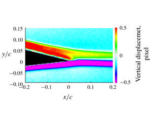
Figure 2 shows a typical two-dimensional field of the vertical pixel displacement, which is proportional to density gradient from (2.1). The black mask in figure 2 is the airfoil geometry, with surrounding dashed lines indicating the extent of image blur around the airfoil (due to limitations of the optical set-up). Viscous dissipation in the boundary layer, as well as heat transfer from the airfoil, lead to a thermal boundary layer that produces the observed density gradient and vertical deflection. With deflection of light rays away from the airfoil, the upper surface has positive values of displacement and the lower surface has negative displacement values. When the upper and lower boundary layers merge at the trailing edge, this conveniently results in a line of zero displacement that represents the stagnation streakline. This line of zero displacement will be the focus of further analysis as we consider the trailing-edge flow physics.
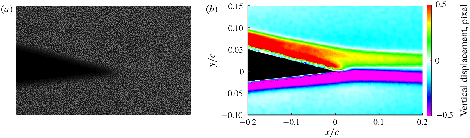
Figure 2. (a) The field of view of the airfoil trailing edge and the background speckle pattern; and (b) the displacement field from cross-correlating BOS images.
3 Results and discussion
3.1 Lift response
The lift response  $C_{l}(t)/C_{l,qs}$ provided by Isaacs’ theory (1.2) is shown by the dashed lines on the right side of figure 3 for $\{k=0.025,\unicode[STIX]{x1D70E}=0.21\}$ and $\{k=0.050,\unicode[STIX]{x1D70E}=0.23\}$. In this representation, the effects of the unsteady dynamic pressure are cancelled through the ratio of the lift coefficients, leaving only the unsteady effects. The unsteady lift response indicated by Isaacs’ theory is due to the influence of shed circulation on the airfoil, producing periodic net downwash or upwash, which affects the induced angle of attack at the airfoil, and thus the lift (see Leishman Reference Leishman2006). (For the present discussion, non-circulatory effects are considered negligible due to the low values of $k$ involved.)
The phase-averaged free-stream Mach number and  $C_{l}(t)/C_{l,qs}(t)$ from experiments are also plotted in figure 3. The time history of Mach number reasonably matches that of the ideal sine wave (1.1), with the $k=0.025$ case providing a better fit. Small deviations from the ideal are visible at the maxima and minima of the Mach time history. The higher reduced frequency case departs from the ideal in a more pronounced manner. This behaviour is likely to be due to the presence of tunnel resonance conditions – the low-frequency case largely avoids resonance, but the $k=0.050$ case is nearing a tunnel resonance frequency (see Zhu et al. Reference Zhu, Harter, Gregory and Bons2018). Owing to the uncertain impact of tunnel resonance, the following analysis focuses on the lower-frequency ( $k=0.025$) case.

Figure 3. (a) Phase-averaged free-stream Mach numbers; and (b) phase-averaged lift frequency responses.
The experimentally measured lift coefficient ratio exhibits significant differences from the theoretical predictions for both reduced frequencies. For the  $k=0.025$ case, the experimental $C_{l}$ reaches a maximum value at $\unicode[STIX]{x1D714}t=135^{\circ }$, compared to the analytical value of $\unicode[STIX]{x1D714}t=229^{\circ }$. Furthermore, the maximum $C_{l}(t)$ is approximately 1.12 times higher than $C_{l,qs}$, compared to Isaacs’ result of 1.02. The minimum $C_{l}(t)$ is approximately 0.92 times the quasi-steady $C_{l}$ and occurs around $\unicode[STIX]{x1D714}t=300^{\circ }$. For the higher-frequency case ( $k=0.050$), much higher overshoot and undershoot in the lift coefficient are observed. At $\unicode[STIX]{x1D714}t=180^{\circ }$ the overshoot reaches a maximum value of 1.29 (compared to 1.04 at $\unicode[STIX]{x1D714}t=238^{\circ }$ indicated by Isaacs), whereas at $\unicode[STIX]{x1D714}t=320^{\circ }$ the maximum undershoot reaches 0.85. Also, for $k=0.050$, a secondary peak in lift overshoot occurs at $\unicode[STIX]{x1D714}t=270^{\circ }$, corresponding to the change in acceleration at the same phase angle in Mach number. For both reduced frequencies, the unsteady lift effects are substantially higher than what is predicted by Isaacs’ theory, and there are significant phase differences between experiment and theory in the prediction of the lift peaks. The results presented here are representative of a wide range of test conditions studied, including variations on reduced frequency, velocity amplitude ratio and airfoil section. Experimental measurements always exhibited greater maximum overshoot and undershoot than the theory, and significant differences in the phase angles at which the maxima or minima occur. These results are at odds with the partial validation provided by Strangfeld et al. (Reference Strangfeld, Müller-Vahl, Nayeri, Paschereit and Greenblatt2016), where the amplitude and phase of $C_{l}(t)$ more closely matched those of Isaacs when the suction surface boundary layer was tripped.
3.2 Stagnation streakline and the Kutta condition
Given the significant lack of agreement between Isaacs’ theory and these high- $Re$ experimental results, it is important to re-evaluate the assumptions employed by unsteady-airfoil theory. Even though these experimental conditions are within the range of parameters where the classical Kutta condition has generally been accepted (fixed pitch, low $\unicode[STIX]{x1D6FC}$, low $k$, low $\unicode[STIX]{x1D70E}$, high $Re$), the validity of the Kutta condition is a key question to be addressed. The details of the trailing-edge stagnation condition are evaluated through field measurements of the immediate trailing-edge region.
The BOS results provided in figures 2 and 4 show contours of the vertical displacement field measured by BOS, which are proportional to  $\unicode[STIX]{x2202}\unicode[STIX]{x1D70C}/\unicode[STIX]{x2202}y$. Positive displacement for the suction-side boundary layer and negative displacement for the pressure-side boundary layer merge at the trailing edge, where the stagnation streakline forms and is indicated by zero displacement. If the classical Kutta condition holds true, the stagnation streakline would initiate at the trailing edge, depart at an angle that bisects the trailing-edge angle, and have a fixed angle that is independent of velocity. However, figure 4 for $k=0.025$ clearly shows that the trailing-edge angle is not bisected, and that the stagnation streakline oscillates in the transverse direction as a function of $U(t)$.

Figure 4. Snapshots of the BOS displacement field at selected phase angles for  $k=0.025$.
The steady and phase-averaged unsteady trailing-edge stagnation streaklines are further examined in figure 5. The steady stagnation streamline does not bisect the trailing edge; instead, it curves up after the trailing edge and gradually flattens out further downstream of  $x/c=0.05$. This may be due to the finite $\unicode[STIX]{x0394}p$ encountered at the trailing edge of the airfoil, resulting from viscous effects (see Bisplinghoff et al. Reference Bisplinghoff, Ashley and Halfman1996; Taha & Razaei Reference Taha and Razaei2019). There may also be a very small region of reversed flow forming at the trailing edge, with streamline curvature occurring in order to balance the momentum. For the unsteady free stream, the trailing-edge stagnation streaklines show significant movement. Both the curvature and position of the streaklines vary with phase angle, especially close to the trailing edge (for $x/c\leqslant 0.05$). The oscillation of the stagnation streakline is indicative of a moving stagnation point, where a downward movement of the stagnation point leads to a higher $C_{l}$, and vice versa. Based on the data shown in figure 5, the maximum distance between the unsteady streaklines and the steady stagnation streamline is plotted as $(h-h_{steady})/c$ in figure 6 for all phase positions. There is a clear transverse movement of the stagnation streakline, with a magnitude of $|h_{max}-h_{min}|/c\approx 5\times 10^{-3}$. This streakline movement can be considered an effective cambering or decambering of the airfoil, with a resulting impact on $C_{l}(t)$. Both the magnitude and phase of the streakline movement (figure 6) are commensurate with an effective camber effect on the observed lift fluctuations (figure 3).

Figure 5. Trailing-edge stagnation streakline oscillations captured from the BOS displacement field at selected phase angles for  $k=0.025$.

Figure 6. Effective camber effect for  $k=0.025$.
3.3 Discussion
The BOS data clearly demonstrate that the classical Kutta condition is violated in this unsteady surging flow. The steady Kutta condition effectively captures all viscous effects for implementation in thin-airfoil theory, but the assumption is inappropriate for unsteady surging flows since it leads to significant error in the predicted magnitude and phase of the unsteady lift response. This result is somewhat surprising, since the general consensus formed in the body of the literature (Ho & Chen Reference Ho, Chen, Michel, Cousteix and Houdeville1981; McCroskey Reference McCroskey1982; Crighton Reference Crighton1985) indicated that the classical Kutta condition could safely be applied in low- $\unicode[STIX]{x1D6FC}$, low- $k$, low- $\unicode[STIX]{x1D70E}$ and high- $Re$ surging flow conditions with a fixed airfoil. At the same time, the result should not be surprising – shedding of circulation in the wake originates from the boundary layers (Bisplinghoff et al. Reference Bisplinghoff, Ashley and Halfman1996), and time-varying boundary layer behaviour allows for a pressure discontinuity at the trailing edge (Taha & Razaei Reference Taha and Razaei2019). Thus, Isaacs’ simultaneous imposition of the classical Kutta condition and shedding of vorticity in the wake is an inherent contradiction. The present findings show that the violation of the classical Kutta condition produces a non-negligible impact on $C_{l}(t)$, where movement of the trailing-edge stagnation point dominates Isaacs’ effect of induced upwash or downwash from shed vorticity.
The precise reason for the violation of the classical Kutta condition is not yet clear. However, it may be due to the momentum balance at the trailing edge, where the net induced velocity from the shed circulation interacts with the boundary layers and trailing-edge shear layer to force movement of the rear stagnation point (Xia & Mohseni Reference Xia and Mohseni2017; Taha & Razaei Reference Taha and Razaei2019). For instance, when clockwise vorticity is present in the near wake, the induced upward velocity at the airfoil will couple with the momentum imbalance of the upper and lower boundary layers to force the stagnation point upwards and decrease  $C_{l}$ relative to $C_{l,qs}$. Likewise, the induced downward velocity from anticlockwise shed circulation would force the stagnation point downwards and increase $C_{l}$.
This perspective could also harmonize the findings of Strangfeld et al. (Reference Strangfeld, Müller-Vahl, Nayeri, Paschereit and Greenblatt2016) with the present work. In Strangfeld et al.’s work, there was an asymmetry in the implementation of boundary layer trips on the upper and lower surfaces of the airfoil. This may have resulted in significant asymmetry of the boundary layer characteristics between the upper and lower surfaces, which would affect susceptibility to separation, as well as the nature of the momentum balance at the trailing edge. Their trailing-edge flow streamlines may have been biased in a particular direction due to the boundary layer asymmetry, leading to the significant differences observed when the airfoil was positioned at positive or negative angle of attack.
4 Conclusion
The aim of this work was to perform a high- $Re$ validation of Isaacs’ theory for unsteady lift production on an airfoil in a surging free stream. Unlike previous, lower- $Re$ experiments that partially validated the theory (Strangfeld et al. Reference Strangfeld, Müller-Vahl, Nayeri, Paschereit and Greenblatt2016), the present results exhibited significant differences in magnitude and phase between experimental results and the theory, as indicated by time histories of $C_{l}(t)/C_{l,qs}(t)$. A detailed study of the trailing-edge flow using background-oriented schlieren showed that the trailing-edge stagnation streaklines move significantly in the transverse direction during a cycle of the unsteady velocity time history. This clearly demonstrates that the classical Kutta condition is not valid for this surging flow case, even when the relevant parameters of reduced frequency, velocity amplitude ratio, angle of attack and Reynolds number otherwise satisfy thin-airfoil theory assumptions. Both the magnitude and phase of the observed movement of the trailing-edge stagnation point are commensurate with the observed $C_{l}(t)$, with stagnation-point movement dominating the inviscid upwash/downwash effects modelled by Isaacs’ theory.
Acknowledgements
This project was funded by Army Research Office grant W911NF-17-1-0110, Unsteady Compressibility Effects for Modern Rotorcraft, monitored by Dr M. Munson. The authors also wish to thank G. Altamirano, M. Azese, B. Harter, D. Pitts and B. Ritchie for their helpful comments and input throughout the development of this work.
Declaration of interests
The authors report no conflict of interest.


 Open access