1. INTRODUCTION
Integrated Global Navigation Satellite Systems (GNSS) and Inertial Navigation Systems (INS) have been widely used in various applications in navigation. INS are self-contained systems which use gyros and accelerometers to provide accurate navigation information (i.e., position, velocity, and attitude) over the short term, while GNSS have bounded errors and can provide long-term accurate position and velocity in ideal conditions (Titterton and Weston, Reference Titterton and Weston2004). These two systems are integrated to provide accurate and reliable navigation information. In such integration, the GNSS-derived position and velocity is often used to update information through a Kalman Filter (KF) while the Inertial Measurement Unit (IMU) provides navigation information during GNSS signal outages and is used for quick GNSS signal reacquisition (Niu et al., Reference Niu, Nassar and El-Sheimy2007).
Traditional INS devices are bulky, expensive and complex, and are not suitable for general land navigation applications (Han and Wang, Reference Han and Wang2010). Recent advances in the construction of Micro Electro-Mechanical Systems (MEMS) devices have made the manufacture of small and light inertial navigation systems possible (Woodman, Reference Woodman2007). MEMS inertial sensors are small and lightweight, and have low power consumption, which makes them attractive candidates for INS/GNSS integrated systems (Syed et al., Reference Syed, Aggarwal, Goodall, Niu and El-Sheimy2007).
However, MEMS inertial sensors suffer from various errors including deterministic and stochastic errors (Nassar, Reference Nassar2003). The impact of deterministic errors on navigation is significant because any small acceleration or angular velocity errors can be integrated into increasing attitude, velocity and position errors; therefore only when the majority of deterministic errors are removed can the MEMS INS be used to provide accurate and reliable navigation information.
Calibration is known as a fundamental way of removing the majority of deterministic errors in inertial sensors and IMUs; however, for low-cost sensors such as MEMS, sensor errors are highly dependent on environment factors such as temperature changes (Aggarwal et al., Reference Aggarwal, Syed, Niu and El-Sheimy2008b). More explicitly, the actual values of sensor errors vary from those obtained through the calibration process due to the difference between the operational and calibration temperatures (Naranjo, Reference Naranjo2008). Such errors, if not compensated for, will accumulate and lead to attitude and position drifts. Approximately, for 2-D navigation, an uncompensated gyro bias will introduce an attitude error proportional to the elapsed time, and a position error proportional to time cubed; also, the uncompensated bias and scale factor error of an accelerometer will introduce a position error proportional to time squared. To compensate for these errors, it is necessary to investigate the thermal characteristics of sensor errors (Syed et al., Reference Syed, Aggarwal, Goodall, Niu and El-Sheimy2007).
In this paper, a reliable thermal calibration procedure is designed and used to investigate the thermal characteristics of MEMS IMUs over the full operational temperature range. Test results reveal several key thermal characteristics of MEMS inertial sensors, such as significant parameter drifts with temperature changes, the inconsistencies under different temperature changing profiles, and the need for periodical recalibration of the thermal drift parameters. This paper also provides a balanced strategy by using the sensor data during both heat-and-stay and cool-and-stay processes to ease the inconsistency issue. With the proposed strategy, reliable thermal error models of two typical MEMS IMUs were established and their contribution was further verified by both the thermal compensation and navigation tests.
This paper is organised as follows: Section 2 reviews previous works and states the problem; Section 3 introduces the proposed thermal calibration procedure; Section 4 describes the tests, including the thermal calibration tests, the compensation tests, and the navigation tests as well as the results analysis; Section 5 provides conclusions.
2. PREVIOUS WORKS
To reduce or eliminate the impact of deterministic IMU errors, various calibration approaches are designed according to the grade of IMUs and applications (Shin and El-Sheimy, Reference Shin and El-Sheimy2002; Syed et al., Reference Syed, Aggarwal, Goodall, Niu and El-Sheimy2007; Fong et al., Reference Fong, Ong and Nee2008; Nieminen et al., Reference Nieminen, Kangas, Suuriniemi and Kettunen2010; Zhang et al., Reference Zhang, Wu, Wu, Wu and Hu2010; Li et al., Reference Li, Niu, Zhang, Zhang and Shi2012). However, in real-world missions, the IMUs may be exposed to various conditions and sensor errors are susceptible to environmental factors, especially the temperature. To compensate for the thermal drifts of sensor errors, thermal calibration methods are proposed. There are currently two thermal calibration approaches: the Soak method and the Ramp method. The Soak method works on the premise of stable sensor temperature while the Ramp method is based on time-varying sensor temperature.
In the Ramp method, the IMU is controlled to continuously execute a sequence of calibration actions under changing temperatures. The Ramp method is more efficient in principle because it does not need the process of stabilising the sensor temperature inside the IMUs (Berman, Reference Berman2011; Reference Berman2012) However, there are two main issues inherent in the Ramp method, especially when it is used for the calibration of IMUs, instead of sensors. One is that there are temperature differences between the inertial sensors and temperature sensor inside the IMUs because they have different cores. Thus, what we can get is the temperature at the core of temperature sensor, not that of inertial sensors. The other issue is that the chamber temperature changes during the calibration process will lead to changes in sensor errors, which in turn causes the calibration errors because the raw sensor data is not collected at the same temperature. This also explains why the temperature stabilisation process is needed in the Soak method.
In the Soak method, the temperature is controlled to be stable at several typical temperature points. Compared to the Ramp method, the Soak method needs more time since the temperature stabilisation process is time-consuming. Even so, the Soak method is the most commonly used method and has shown effectiveness in both the calibration of deterministic errors and the modelling of stochastic errors (Shcheglov et al., Reference Shcheglov, Evans, Gutierrez and Tang2000; Abdel-Hamid, Reference Abdel-Hamid2004; El-Diasty et al., Reference El-Diasty, El-Rabbany and Pagiatakis2007; Aggarwal et al., Reference Aggarwal, Syed and El-Sheimy2008a; Niu et al., Reference Niu, Li, Zhang, Wang and Ban2013). This is because the Soak method can provide the most reliable values of sensor errors at the chosen temperature points by stabilising the temperature.
Therefore, the choice of the thermal calibration method is a trade-off between accuracy and cost. Since both thermal calibration methods have been shown to be useful in improving the performance of inertial sensors, one can choose an appropriate method according to requirement and cost. As our purpose is to investigate the thermal characterisation of inertial sensors, we need a more stable method to reduce the errors introduced by the calibration method. Therefore, the Soak method is used. In this paper, a whole thermal calibration procedure is designed to study the thermal drifts of a full set of sensor errors within the entire operational range. The principles of designing the calibration procedure, including the design of calibration scheme, the estimation of sensor errors, the establishment of thermal models, etc., are described in detail. This calibration procedure is then used to establish the thermal models of two typical MEMS IMUs.
It is found from these tests that the thermal drifts of MEMS sensor errors are related to not only the current temperature but also the previous temperature changing history. That is, with various temperature changing profiles, the thermal models for the sensor errors can be different. Since our calibration procedure has been tested to be reliable, such an inconsistency might come from the inherent property of the MEMS inertial sensors. The existence of such inconsistency posed a challenge to the following assumption of thermal calibration: the thermal drift of a sensor error is only related to the temperature of the sensor core. In practical applications, there are innumerable temperature scenarios; however, it is impossible to consider all the possible temperature profiles during the in-lab thermal calibration stage. This paper mitigates this issue by using a balanced strategy that makes comprehensive use of the sensor measurements during both heat-and-stay and cool-and-stay processes. The thermal models established through this strategy have been proved to be robust to enhance all sensors and navigation states (i.e., attitude, velocity, and position).
3. THERMAL CALIBRATION AND COMPENSATION PROCEDURE
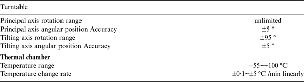
In this section, the procedure, including the design of the calibration scheme, the estimation of sensor errors and the establishment of thermal models are described. The proposed procedure is based on a dual-axis position turntable integrated with a thermal chamber (as shown in Figure 1). The performance characteristics of both the turntable and the thermal chamber are shown in Table 1. The turntable is accurate enough to provide a reference for the calibration of low-grade IMUs. Also, there are high-precision locating pins on the mounting plate of the turntable to keep the IMUs' axes aligned with the turntable axes.

Figure 1. Thermal calibration equipment.
Table 1. Specifications of calibration equipment.
3.1. Design of the calibration scheme
One basic principle for the calibration scheme design is to install the IMUs only once. Moreover, the scheme should allow every accelerometer axis to point up and down precisely and the IMU to be rotated around every gyro axis both clockwise and counter-clockwise with known angles. Considering both characteristics of the equipment and calibration efficiency, the following eight-step calibration scheme is designed (as shown in Figure 2).
Figure 2. IMU actions in an eight-step calibration scheme.
There are eight static positions and eight rotations in one calibration scheme. The IMU outputs at eight static positions are used to calibrate all accelerometer errors and gyro biases, while those during the eight rotation processes are utilised to estimate gyro scale factors and non-orthogonalities.
It is vital to reduce the impact of sensor noises. For static positions, the effect of noises can be reduced through averaging the sensor outputs. Since there are eight static positions, the gyro noises can cause calibration errors of gyro biases
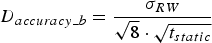 $$D_{accuracy\_b} = \displaystyle{{\sigma _{RW}} \over {\sqrt 8 \cdot \sqrt {t_{static}}}} $$
where σ RW is the angular random walk (ARW) coefficient,  $D_{accuracy\_b} $ is the desired gyro biases estimation accuracy, t static is the static time. Similarly, the accelerometer calibration errors caused by noises can be computed.
To calibrate gyro scale factors and non-orthogonalities with the position turntable, the gyros' outputs are integrated to get the angles of rotation. This integration will result in the accumulation of gyro noises. Therefore it is preferred to perform the rotation at a higher rate to reduce the impact of noises. Since each axis experiences at least two rotations in one calibration scheme, the calibration errors of gyro scale factors or non-orthogonalities caused by gyro noises can be computed by Equation (2).
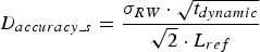 $$D_{accuracy\_s} = \displaystyle{{\sigma _{RW} \cdot \sqrt {t_{dynamic}}} \over {\sqrt 2 \cdot L_{ref}}} $$
where L ref is the true rotation angle and is 90° here,  $D_{accuracy\_s} $ is the desired gyro scale factors and non-orthogonalities estimation accuracy, t dynamic is the dynamic time, and σ RW is the ARW coefficient.
3.2. Sensor Error Models and Estimation of Sensor Errors
The error models of accelerometers and gyros can be written as
 $$\delta {\rm \bf f} = {\rm \bf b}_a + {\rm \bf S}_a {\rm \bf f} + {\rm \bf N}_a {\rm \bf f} + {\rm \bf v}_a $$
 $$\delta {\rm \bf \omega} = {\rm \bf b}_g + {\rm \bf S}_g {\rm \bf \omega} + {\rm \bf N}_g {\rm \bf \omega} + {\rm \bf v}_g $$
where  $\delta {\rm \bf f}$ and $\delta {\rm \bf \omega} $ are the error vectors of the accelerometer-derived specific forces and the gyro-derived angular velocity, f and ${\rm \bf \omega} $ are the true specific forces and angular velocity, ba and bg are accelerometer and gyro biases, Sa and Sg are the diagonal matrices containing the scale factor errors, Na and Na are the skew-symmetric matrices containing the non-orthogonalities and va and vg represent the noises.
The accelerometer errors are estimated with least-squares, while the gyro errors are calculated through a two-step method (Li et al., Reference Li, Niu and Zhang2011). The details of calibration computations are shown in the Appendix.
3.3. Establishment of thermal models
To compensate for the thermal drifts of sensor errors, continuous global compensation models must be developed. In real-world tests with various MEMS sensors, we found that some sensor errors cannot be fitted to polynomial models because of the sharp wiggles at certain temperatures. Therefore the first-order piecewise function is introduced to establish the thermal models
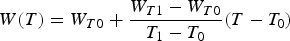 $$W(T) = W_{T0} + \displaystyle{{W_{T1} - W_{T0}} \over {T_1 - T_0}} (T - T_0 )$$
where T is a temperature between T 0 and T 1. W(T) is the calculated sensor error at T, W T0 and W T1 are the sensor errors at temperature T 0 and T 1. The established thermal models can be used to calculate the sensor errors (or the thermal drifts) at each temperature and then remove them from the IMU outputs.
4. TESTS AND RESULTS
This section describes the tests, including thermal calibration tests, thermal compensation tests and navigation tests. The proposed procedure was first applied to build thermal models of two typical MEMS IMUs in the thermal calibration tests. With the established thermal models, thermal compensation tests were implemented to investigate the effect of thermal compensation on inertial sensors. Then navigation tests with static IMU data were performed to study the effect of the thermal compensation on the navigation solutions.
4.1. IMUs used in the tests
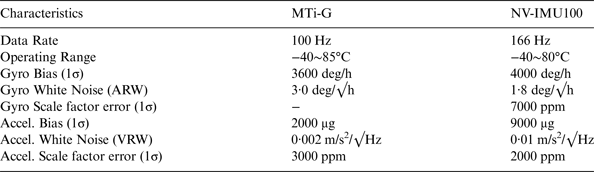
The two IMUs tested are Xsens MTi-G (Xsens, 2014) and NV-IMU100 (NAV Technology, 2014). Their appearances and related characteristics are illustrated in Figure 3 and Table 2. The raw output of MTi-G (without factory compensation) was used. The NV-IMU100 has three MEMS vibrating ring gyros, and its output data had been partly compensated after factory calibration.
Figure 3. Two MEMS IMUs Tested (mounted on table top inside thermal chamber).
Table 2. Specifications of tested IMUs.
4.2. Thermal calibration tests and results
The thermal calibration process followed the procedure described in Section 3. Both the heat-and-stay and the cool-and-stay temperature profiles were implemented to investigate the thermal characteristics of inertial sensors under different temperature changing conditions. The chamber temperature was controlled to increase from −10 °C to +70 °C with 20 °C steps (heat-and-stay) and then decrease from +70 °C to −10 °C with −20 °C steps (cool-and-stay). At each step, the temperature was kept stable for an hour. Also, to test the proposed calibration procedure and the repeatability of sensor errors under the same temperature changing condition, both the heat-and-stay and the cool-and-stay temperature profiles were repeated three times.
4.2.1. Thermal calibration Results of MTi-G
The results of MTi-G are shown in Figure 4. The sensor errors at the chosen temperature steps were shown as the nodes on the curves, while those at other temperature points were obtained with linear interpolation and illustrated by lines. The dashed and solid lines represent the results with the cool-and-stay profile and those with the heat-and-stay profile, respectively. We found that all the sensor errors had repeatable curves during the three tests with the same temperature conditions. Therefore we only show all the results of biases to illustrate the repeatability. Only one set of results is shown for the scale factor errors and non-orthoganility errors to make the figures clear.
Figure 4. Calibration results of MTi-G. In each figure, the dashed lines are the results with the cool-and-stay temperature changing profile and the solid lines are the results with the heat-and-stay temperature changing profile.
As shown in Figure 4, sensor errors, not only biases, but also scale factor errors and non-orthogonalities, varied significantly with temperature. The change of gyro biases reached approximately 1500 °/h for z-axis and several hundred °/h for both x- and y-axis. Meanwhile, the change of accelerometer biases reached 3000 µg over the entire temperature range. The changes of the scale factors and non-orthogonalities could also be several thousand parts per million (ppm). These changes reveal the temperature sensitive characteristic of MEMS sensors.
Moreover, it is notable that the MEMS sensor errors had repeatable values at the same temperature points during tests with the same temperature profile, which also indicates the reliability of the thermal calibration procedure. However, some sensor errors showed significant inconsistencies under different temperature profiles. For example, the y-axis gyro bias and the x-axis accelerometer bias had an inconsistency of 1000 °/h and 3000 µg, respectively. As the Soak method can provide very reliable thermal calibration results (which can also be verified by the results with the same temperature profile), the inconsistencies under different temperature conditions are probably an issue inherent in MEMS sensors.
4.2.2. Thermal calibration results of NV-IMU100
The calibration results of NV-IMU100 are shown in Figure 5. The gyro biases were small (less than 10 °/h) due to the symmetry of vibrating ring gyros and the factory compensation. However, the change of gyro scale factors (e.g., y-axis) exceeded 10000 ppm. These characteristics matched the inherent feature of the vibrating ring gyros. For accelerometers, the changes reached 13000 µg for biases, and 4000 ppm for scale factors. There were also inconsistencies between the curves of some sensor errors under different temperature profiles. For example, both the x- and z-axis accelerometer biases had an inconsistency of almost 10000 µg, while the y-axis gyro had a difference of 5000 ppm.
Figure 5. Calibration results of NV-IMU100. In each figure, the dashed lines are the results with the cool-and-stay temperature changing profile and the solid lines are the results with the heat-and-stay temperature changing profile.
Results of the thermal calibration tests indicated that MEMS sensor errors varied significantly with temperature. Furthermore, sensor errors might have significant inconsistent curves under different temperature changing profiles. To mitigate the issue of inconsistencies and get a reliable thermal model, the results from the heat-and-stay and cool-and-stay processes at the same temperature points were averaged to provide the final results. The established thermal models were utilised to compensate for the thermal drifts in both the thermal compensation and the navigation tests.
4.3. Thermal compensation tests and results
The impact of thermal compensation was investigated by comparing the residual errors (i.e., the difference between the sensor outputs and the inputs) in three test modes.
Mode #1: without thermal compensation.
Mode #2: after compensation with the cooling models (i.e., the thermal models built under the cool-and-stay temperature profile). The cool-and-stay temperature profile was significantly different from the actual temperature condition in these tests. Therefore this test model represented the compensation tests with the thermal models obtained under a temperature profile that is inconsistent with the actual one.
Mode #3: after compensation with the averaged models (i.e., the thermal models built by averaging the results from the heat-and-stay and cool-and-stay processes).
Tests with similar temperature profiles were not conducted here. They were expected to provide the best results because of the repeatability of sensor errors under the same temperature condition; however, it is impossible to consider all the possible temperature profiles in practical uses during the thermal calibration stage.
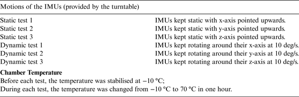
There were six tests, including three static tests and three dynamic tests, as described in Table 3. For each test the environment temperature was changed from −10 °C to +70 °C with a profile that is different from that during the thermal calibration tests, and the turntable was used to provide known sensor inputs. Each test focused on one sensor that experienced the motion from the turntable. For example, the x-axis accelerometer output was investigated with a reference input of the local gravity in Static test 1, while the x-axis gyro output was studied with a reference input of 10 °/s in Dynamic test 1. The IMU outputs were averaged during each second to mitigate the impact of the sensor noises.
Table 3. Descriptions of the six thermal compensation tests.
4.3.1. Thermal compensation results of MTi-G
Figure 6 shows the compensation results of MTi-G. Each subplot shows the result of one sensor in the corresponding test. The blue, green, and red lines are the residual errors in Mode #1, #2, and #3, respectively.
Figure 6. Residual errors in MTi-G outputs.
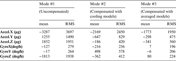
The residual errors in Mode #1 were immense (i.e. reached −3000 °/h and −5000 µg for gyros and accelerometers) and changed with long-term trends; however, after thermal compensation in either Mode #2 or #3, the residual errors were significantly reduced, and the main long-term trends were mitigated. There were still some changes in the y-axis gyro output. Such changes (with a RMS of around 200 °/h) were not significant for MEMS gyros, which might be caused by stochastic errors.
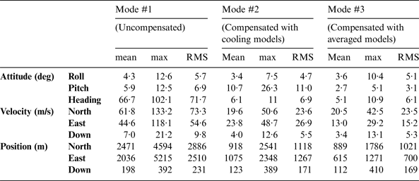
The statistics (i.e., the mean and the RMS values) of the residual errors are shown in Table 4. The RMS values were 3697, 1490 and 1951 µg for accelerometers outputs, and 279, 264 and 1938 deg/h for gyro outputs in Mode #1. After thermal compensation, the RMS values were 1950, 475 and 560 µg, and 196, 206 and 224 °/h in Mode #2, and 1950, 475, and 560 µg, and 196, 206, and 224 °/h in Mode #3. Thus, even the calibration and compensation were conducted under different temperature profiles, the residual errors in most sensors were significantly reduced in Mode #2. However, both the x- and y-axis gyros became worse after compensation in Mode #2. On the other hand, all sensors became better after compensation in Mode #3, which indicated the robustness of compensating with the averaged thermal models.
Table 4. Statistics of residual errors in MTi-G outputs.
4.3.2. Thermal compensation results of NV-IMU100
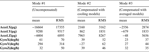
Figure 7 shows the compensation results of NV-IMU100 and Table 5 gives the corresponding statistics. The residual errors were significantly reduced and the long-term changes trends were mitigated after thermal compensation. All sensors were enhanced after compensation in Mode #3. On the other hand, the compensation in Mode #2 enhanced most of the sensors but degraded the z-axis accelerometer.
Figure 7. Residual errors in NV-IMU100 outputs.
Table 5. Statistics of residual errors in NV-IMU100 outputs.
Results show that thermal compensation can be effective in reducing the long-term thermal drifts of sensor errors. However, there is a risk that the residual sensor errors may increase after thermal compensation if the actual thermal condition is different from the calibration temperature profile. Compensating with the averaged thermal model is a feasible way to improve the robustness of thermal calibration.
4.4. Navigation tests and results
The navigation solution (i.e., attitude, velocity, and position) in three test modes (as described in subsection 4.3) were calculated and compared. The pure INS mechanisation was implemented as the algorithm for the three modes. The details of the mechanisation algorithm have been well described in Shin (Reference Shin2005). Also, we set the initial attitude and position manually at the beginning of each segment in the three modes to focus on the impact of sensor errors on the navigation errors. Hence the navigation algorithm (i.e. the pure INS mechanisation) and the initial attitude, velocity and position information are exactly the same except for the sensor outputs compensation. Ten data segments at different temperature points were chosen to run the INS navigation algorithm. Each segment lasted for two minutes. To highlight the effect of thermal compensation, static data was used to eliminate the impact of other factors such as vehicle manoeuvres. The navigation drifts of Mti-G and IMU100 are shown in Figures 8 and 9, respectively.
Figure 8. Navigation drifts of Mti-G.
Figure 9. Navigation drifts of NV-IMU100.
4.4.1. Navigation results of Mti-G
In Figure 8, the maximum drifts of attitude, velocity, and position reached 100°, 130 m/s, and 5000 m in Mode #1. After compensation, these values were reduced to approximately 25°, 50 m/s and 2500 m in Mode #2 and 10°, 40 m/s and 1800 m in Mode #3. To make the comparison clear, the statistics of the drifts are shown in Table 6.
Table 6. Statistics of navigation drifts of Mti-G.
The RMS value of the heading error were reduced from 71·7° in Mode #1 to 6·9° in Mode #2 and 6·1° in Mode #3, which indicates the contribution of thermal compensation. However, the RMS value of the pitch error increased from 6·9° in Mode #1 to 11·0° in Mode #2 because the performance of the y-axis was degraded after compensation with an inaccurate thermal model; this value was reduced to 3·1° in Mode #3. The RMS values of the position drifts in north and east decreased from 2886 and 2510 m in Mode #1 to 1118 and 1267 m in Mode #2, which were further reduced to 1021 and 700 m in Mode #3.
Even after compensation with the averaged models, the maximum attitude, velocity and position errors reached more than ten degrees, several tens of metres per second and more than one thousand metres. This is partly because the established error models cannot eliminate the deterministic sensor errors completely due to the inconsistency of MEMS sensor errors under different thermal profiles. Moreover, some drifts may be caused by residual sensor errors such as run-to-run bias and the noises (e.g. quantisation noises, white noises, angular rate/acceleration random walk noises). In real-world navigation applications, constraints such as non-holonomic constraints (NHC) and odometer measurements are commonly used to correct the inertial navigation solution, which is beyond the scope of this paper.
To summarise, in the attitude estimation level, there was still a possibility of degrading the system performance in Mode #2 due to the inconsistencies of sensor errors under different temperature profiles. However, for positioning, either thermal compensation mode enhanced the system significantly. The results in Mode #3 were more accurate than those in Mode #2 because the thermal models in Mode #3 were more robust.
4.4.2. Navigation results of NV-IMU100
Figure 9 shows the navigation drifts of NV-IMU100, and Table 7 gives the statistics.
Table 7. Statistics of navigation drifts of NV-IMU100.
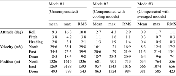
The maximum RMS values of attitude, velocity, and position were reduced from 10·0°, 40 m/s, and 1600 m in Mode #1 to 2·9°, 22 m/s, and 1000 m in Mode #2 and 1·1°, 18 m/s, and 700 m in Mode #3. However, the RMS values of velocity and position in vertical direction were degraded from 9·8 m/s and 543 m in Mode #1 to 20·9 m/s and 984 m in Mode #2. These comparisons further verified the contribution of thermal compensation and the advantage of using the averaged thermal models.
4.5. Importance of periodical calibration
The performance of the tested IMUs was significantly improved after thermal compensation. However, we found that some sensor errors showed significant inconsistent thermal drift curves six months after thermal compensation. Figure 10 shows the Mti-G accelerometer biases and non-orthogonalities in July 2013 (the solid lines) and January 2014 (the dashed lines). Although the surrounding environment of the tests were different (with a room temperature of 30 °C in July 2013 and 10 °C in January 2014), the thermal chamber isolated the IMUs from the external environment and provided the same temperature changing profile (i.e., increasing the temperature from −10 °C to 70 °C with 10 °C steps) for both tests. It is shown that the x-axis accelerometer bias had a repeatability of over 3000 μg in two tests; also, the non-orthogonalities between the x- and y-axis had a repeatability of 2000 ppm. The inconsistencies suggest that periodical thermal calibration is necessary for MEMS IMUs.
Figure 10. Calibration results of two tests with a time interval of six months. Solid and dashed lines are results in July 2013 (the solid lines) and January 2014 (the dashed lines), respectively.
5. CONCLUSIONS
This paper investigates the thermal characteristics of typical MEMS IMUs with a reliable thermal test procedure.
Thermal calibration results show that MEMS sensor errors, not only biases, but also scale factors and non-orthogonalities, can vary significantly with temperature. These sensor errors had repeatable curves during tests with the same temperature profile; however, some of them showed significant inconsistencies at the same temperature points under different temperature profiles. Since our thermal calibration procedure has been tested to be reliable, these inconsistencies are probably an issue inherent in MEMS sensors.
Thermal compensation results indicate that thermal compensation is effective in reducing the long-term residual errors in the sensor outputs; however, there is a risk that the residual sensor errors may increase after thermal compensation if the actual thermal condition is different from the temperature profile for thermal calibration, due to the inconsistencies of MEMS sensor errors motioned above. Since it is impossible to consider all the real-world temperature profiles during the in-lab thermal calibration stage, a feasible way to mitigate this issue is presented by using the sensor data during both heat-and-stay and cool-and-stay processes to establish the averaged thermal models. It was verified that compensating with the averaged thermal models is a robust way to enhance all sensors.
In the navigation tests, even using the thermal models established under a different temperature profile significantly enhanced most navigation states (i.e., attitude, velocity, and position). However, there was still a possibility that the inconsistencies of MEMS sensors might degrade the estimation of some navigation information. Compensating with the averaged thermal models can provide the best performance and improved the estimation of all navigation states.
Also, it is found that MEMS sensor errors may have significantly inconsistent thermal drift curves after a time period such as several months, which suggests that periodical thermal calibration is necessary for MEMS IMUs. The outcome of this paper can promote the better understanding and wider uses of MEMS sensors and IMUs.
ACKNOWLEDGEMENT
The authors would like to thank Yalong Ban, Kunlun Yan and Xin Yang for the helps during the tests. This work was supported in part by the National Natural Science Foundation of China (41174028, 41231174), the Key Laboratory Development Fund from the Ministry of Education of China (618-277176), the National High Technology Research and Develop Program of China (2012AA12A206), and the Fund from China Scholarship Council (201306270139).
APPENDIX ESTIMATION OF THE SENSOR ERRORS WITH ACQUIRED DATA IN AN 8-STEP CALIBRATION SCHEME
A1. ESTIMATION OF ACCELEROMETER ERRORS
The accelerometer outputs can be represented as
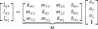 $$\left[ {\matrix{ {l_{ax}} \cr {l_{ay}} \cr {l_{az}} \cr}} \right] = \underbrace {\left[ {\matrix{ {k_{ax}} & {m_{yx}} & {m_{zx}} & {b_{ax}} \cr {m_{xy}} & {k_{ay}} & {m_{zy}} & {b_{ay}} \cr {m_{xz}} & {m_{yz}} & {k_{az}} & {b_{az}} \cr}} \right]}_{\rm M}\left[ {\matrix{ {a_x} \cr {a_y} \cr {a_z} \cr 1 \cr}} \right]$$
where the diagonal elements k ai (i = x, y, z) are the scale factors, the off-diagonal elements m ij (i = x, y, z; j = x, y, z) represent the non-orthogonalities, and b ai (i = x, y, z) are the biases. In the calibration scheme, each accelerometer axis is pointed upward and downward precisely (except z-axis); thus, the ideal specific force can be represented as follows:
 $${\bf a}_{\bf 1} ^{\prime} = \left[ {\matrix{ g \cr 0 \cr 0 \cr}} \right]\,\quad {\bf a}_{\bf 2} ^{\prime} = \left[ {\matrix{ { - g} \cr 0 \cr 0 \cr}} \right]\,\quad {\bf a}_{\bf 3} ^{\prime} = \left[ {\matrix{ 0 \cr g \cr 0 \cr}} \right]\,\quad {\bf a}_{\bf 4} ^{\prime} = \left[ {\matrix{ 0 \cr { - g} \cr 0 \cr}} \right]\,\quad {\bf a}_{\bf 5} ^{\prime} = \left[ {\matrix{ 0 \cr 0 \cr g \cr}} \right]\,$$
Then, the design matrix can be denoted by A and the measured specific forces are denoted by U.
 $${\bf A} = \left[ {\matrix{ {{\bf a}_1 ^{\prime}} & {{\bf a}_2 ^{\prime}} & {{\bf a}_3 ^{\prime}} & {{\bf a}_4 ^{\prime}} & {{\bf a}_5 ^{\prime}} \cr 1 & 1 & 1 & 1 & 1 \cr}} \right]$$
 $${\rm \bf U} = \left[ {\matrix{ {{\rm \bf u}_{\rm \bf 1}} & {{\rm \bf u}_{\rm \bf 2}} & {{\rm \bf u}_{\rm \bf 3}} & {{\rm \bf u}_{\rm \bf 4}} & {{\rm \bf u}_{\rm \bf 5}} \cr}} \right]$$
In this case, the column vector of the U matrix should be:
 $${\bf u}_{\bf 1} = \left[ {\matrix{ {l_{ax}} \cr {l_{ay}} \cr {l_{az}} \cr}} \right]_{X - upwards} \cdot {\bf u}_{\bf 1} = \left[ {\matrix{ {l_{ax}} \cr {l_{ay}} \cr {l_{az}} \cr}} \right]_{X - downwards} $$
u3, u4 and u5 are similar with u1 and u2.Then, the M matrix can be estimated by the least-square method.
 $${\bf M} = {\bf U} \cdot {\bf A}^T ({\bf A} \cdot {\bf A}^T )^{ - 1} $$
A2. ESTIMATION OF GYRO ERRORS
The gyro errors are estimated through a two-step method, instead of using the least-square method directly. The first step is to calculate the biases using static data. The next step is to calculate the scale factor errors and non-orthogonalities with dynamic data.
A2.1. Estimation of gyro biases
The bias of the i-axis gyro can be calculated by:
 $$b_{gi} = \displaystyle{{l_{i - upwards} + l_{i - downwards}} \over 2}$$
where l i-upwards and l i-downwards are the gyro outputs when the axis points upwards and downwards, respectively.
A2.2. Estimation of gyro scale factor errors
The scale factor errors of the i-axis (i = x, y, z) gyro can be estimated using the same idea as the 6-position method.
 $$S_{gi} = \displaystyle{{L_{i - clockwise} - L_{i - anticlockwise}} \over {2L_{ref}}} - 1$$
where S gi is gyro scale factor, L i−clockwise and L i−anticlockwise represent the angle derived by the integration of the i-axis gyro outputs when the IMU is rotated around this axis by L ref clockwise and counter-clockwise, respectively. For the designed 8-step calibration scheme, the value of L ref is 90°.
A2.3. Estimation of gyro non-orthogonalities
The non-orthogonalities cause each axis to be affected by the signal of the other two axes. When the turntable is rotated around i-axis, the output of j-axis will be affected by this rotation due to the non-orthogonalities between i- and j-axis. Thus, the non-orthogonalities between i- and j-axis can be estimated by
 $$n_{ij} = \displaystyle{{L_{{\rm j} - clockwise} + L_{{\rm j} - anticlockwise}} \over {2L_{ref}}} - 1$$
where n ij is the non-orthogonalities of i-axis to j-axis.