


I. INTRODUCTION
Due to photographic equipment limitations, there exist many grayscale images in both the past and present, such as legacy photos, infrared images [Reference Limmer and Lensch1], thermal images [Reference Qayynm, Ahsan, Mahmood and Chcmdary2], radar images [Reference Song, Xu and Jin3], and electron microscope images [Reference Lo, Sim, Tso and Nia4]. These images can be made more vivid and appealing by colorizing them. A user can utilize image tools to manually colorize the objects in the grayscale image, such as blue skies, black asphalt, and green plants, based on empirically conjecture for the suitable color. However, the manual colorizing procedure is laborious and time-consuming, making the job considerably more difficult if the user is unfamiliar with these objects.
Colorization is recent active research yet a difficult subject in the realm of image processing, with the goal of quickly predicting and colorizing grayscale images by analyzing image content with a computer. Existing colorizing algorithms can be classified into three categories depending on the information provided by humans: scribble-based [Reference Levin, Lischinski and Weiss5–Reference Zhang, Li, Wong, Ji and Liu10], example-based [Reference Welsh, Ashikhmin and Mueller11–Reference Lee, Kim, Lee, Kim, Chang and Choo15], and learning-based [Reference Limmer and Lensch1–Reference Lo, Sim, Tso and Nia4, Reference Kuo, Wei and You16–Reference Vitoria, Raad and Ballester32] methods.
The scribble-based methods require a user to enter scribbles into a computer to instruct the colorization algorithm. The user draws correct color scribbles for the textures of various objects in grayscale images, and then the computer automatically propagates the colors of the scribbles to the pixels with the same texture. Levin's method [Reference Levin, Lischinski and Weiss5] developed a quadratic cost function under the assumption that neighboring pixels having similar luminance should also have similar colors. They used this function with color scribbles to produce fully colorized images, but there exists a color bleeding problem in these results. Based on [Reference Levin, Lischinski and Weiss5], Huang et al. [Reference Huang, Tung, Chen, Wang and Wu6] solved this problem by incorporating adaptive edge detection to enhance the boundaries of objects in images. Yatziv and Sapiro [Reference Yatziv and Sapiro7] used the distance between the pixel and its surrounding scribbles to determine the color of the pixel. [Reference Zhang8–Reference Zhang, Li, Wong, Ji and Liu10] used convolutional neural network (CNN) to colorize grayscale images using color provided by color scribbles.
The example-based methods must be provided with pre-screened reference color images that have similar features as the grayscale images to assist in colorizing the grayscale images. [Reference Welsh, Ashikhmin and Mueller11] converted the color space of pre-selected reference color images from RGB to Lab, and then analyzed and compared the luminance channel in its Lab color space with the grayscale image to be colorized, and provided the corresponding chroma information to the grayscale image based on similarities in textures. Gupta et al. [Reference Gupta, Chia, Rajan, Ng and Zhiyong12] used super-pixel segmentation to reduce the computational complexity of [Reference Welsh, Ashikhmin and Mueller11]. [Reference He, Chen, Liao, Sander and Yuan14] proposed a CNN-subnet technique with two CNN sub-nets: a similarity sub-net and a colorization sub-net. It uses the similarity sub-net to build bidirectional similarity maps between a grayscale image and a source image, then utilizes the colorization sub-net to generate a colorized image. [Reference Lee, Kim, Lee, Kim, Chang and Choo15] designed a spatially corresponding feature transfer module that uses self-attention to learn the relationship between the input sketch image and the reference image. Although scribble-based and example-based methods can save a large amount of time when compared to all-manual colorizing, each processed image must still be assisted by providing relevant color information. In addition, the colorizing performance is greatly influenced by the color scribbles and the selected reference image used.
In contrast to the above methods, the learning-based methods just require grayscale images to be fed into a CNN for automatic color image generation. The CNN requires a large number of images to train neural network parameters by analyzing the features of grayscale images to produce appropriate chroma components. The existing learning-based methods convert the color space of images from RGB to YUV or to Lab color space during the training of the CNN to learn the correlation between luminance and chrominance in the images. [Reference Varga and Szirányi17, Reference Larsson, Maire and Shakhnarovich18] both used the pre-trained VGG [Reference Simonyan and Zisserman33] to extract features from grayscale images. Varga and Szirányi [Reference Varga and Szirányi17] utilized the features to predict chroma component for each pixel, while Larsson et al. [Reference Larsson, Maire and Shakhnarovich18] used them to predict the probability distributions of chroma component. [Reference Cheng, Yang and Sheng19–Reference Iizuka, Simo-Serra and Ishikawa23] incorporated semantic labels into the training of colorization models, such as object registration [Reference Cheng, Yang and Sheng19–Reference Zhao, Han, Shao and Snoek22] and scene classification [Reference Iizuka, Simo-Serra and Ishikawa23]. [Reference Qin, Cheng, Cui, Zhang and Miao20–Reference Iizuka, Simo-Serra and Ishikawa23] used two parallel CNNs to solve colorization task and semantic task, respectively, and the colorization task exploits the features extracted from the semantic task to improve colorization performance. [Reference Cheng, Yang and Sheng24] designed a set of networks, each of which aims to colorize a specific class of object. They classified the objects in images first and then colorized them with the matching network. Zhang et al. [Reference Zhang, Isola and Efros25] proposed a learning-based approach regarding color prediction as a classification problem. [Reference Zhang, Isola and Efros25, Reference Mouzon, Pierre and Berger26] classified the ab-pairs of the Lab color space into 313 categories and generated ab-pairs according to the features in images. As human eyes are less sensitive to chrominance, Guadarrama et al. [Reference Guadarrama, Dahl, Bieber, Norouzi, Shlens and Murphy27] employed the PixelCNN [Reference Van den Oord, Kalchbrenner, Espeholt, Vinyals and Graves34] architecture to generate delicate low-resolution chroma components pixel by pixel, and then improved image details with a refinement network. The PixelCNN used in [Reference Guadarrama, Dahl, Bieber, Norouzi, Shlens and Murphy27] will increase the accuracy but it is an extremely time-consuming process.
[Reference Deshpande, Lu, Yeh, Jin Chong and Forsyth28–Reference Vitoria, Raad and Ballester32] made the prediction based on generative adversarial networks (GAN) [Reference Goodfellow35] and GAN variants. Cao et al. [Reference Cao, Zhou, Zhang and Yu30] replaced the U-net of the original generator with a convolutional architecture without dimensionality reduction. All of the aforementioned learning-based colorization methods do not require human assistance and produce faster colorizing results than the other two categories of approaches, but a common problem among them is the resulting images are subdued and have a low saturation in color. In addition, existing neural network-based algorithms often designed complex network architectures to achieve more delicate results, resulting in models with huge parameter counts that are challenging to apply to real-world applications.
The pyramid concept in image processing is to exploit multiple scales of features to make a more accurate prediction, which has recently been used in convolution neural networks [Reference Lin, Dollár, Girshick, He, Hariharan and Belongie36, Reference Zhao, Shi, Qi, Wang and Jia37]. [Reference Lin, Dollár, Girshick, He, Hariharan and Belongie36] combined features from different scales by nearest neighbor up-sampling the lower scale features and then fusing them with the higher scale features. These multi-scale features are extracted from different layers of the backbone convolution neural networks. The results are predicted individually for each scale to ensure that the features at each scale are meaningful. [Reference Zhao, Shi, Qi, Wang and Jia37] implemented different sizes of down-sampling and $1 \times 1$ convolutions on the features obtained in the last layer of the backbone neural networks, and then up-sampled these results to original size before making final predictions based on the concatenation of these modified features and original features.
The objective of our paper is to overcome the aforementioned problem using a fully automatic colorization algorithm based on the learning method. To allow a model to accurately predict chroma information without human hints while also minimizing the difficulty of model training at the same time, we adopted a coarse-to-fine generation approach. Our method is composed of two stages: preliminary chroma map generation and chroma map refinement. We predicted preliminary chroma components by the low-resolution chroma map generation network (LR-CMGN), aiming to obtain coarse color information from grayscale images first, allowing the model to converge more quickly. Then, to enhance the quality of generated chroma map, we generated a high-resolution color image by the refinement colorization network (RCN), which is designed with a pyramid model to reduce the number of model parameters. It is worth noting that we adopted the HSV color space in our method since we observed that machine learning behaves more like humans in this color space and can learn better color and saturation than other color spaces commonly used in this research area, such as Lab and YUV. The contributions in this paper are listed as follows:
• We presented a pyramidal structure of CNNs that predict the images of chroma components H and S in the HSV color space.
• The pyramidal structure can reduce the computing load of the model by analyzing smaller sizes of features and generate more reasonable chroma maps by analyzing information at multiple scales.
• The new loss function is designed for the properties of the H component of the HSV color space, ensuring that the colorized image obtains superior color and saturation.
II. PROPOSED METHOD
In this section, we introduce our colorization method. We first explain why we adopt the HSV color space instead of the YUV and Lab color spaces. The LR-CMGN and RCN architectural designs, as well as their training methodologies, are then detailed. Our colorization procedure, as illustrated in Fig. 1, involves two sub-networks: the LR-CMGN and the RCN, and is carried out in the HSV color space. The V component of HSV is used as a grayscale image for the LR-CMGN input and then generates low-resolution chroma maps. Afterwards, multiple scales of grayscale images and chroma maps are sent into the RCN, which outputs detailed chroma maps and, finally, the colorized image.
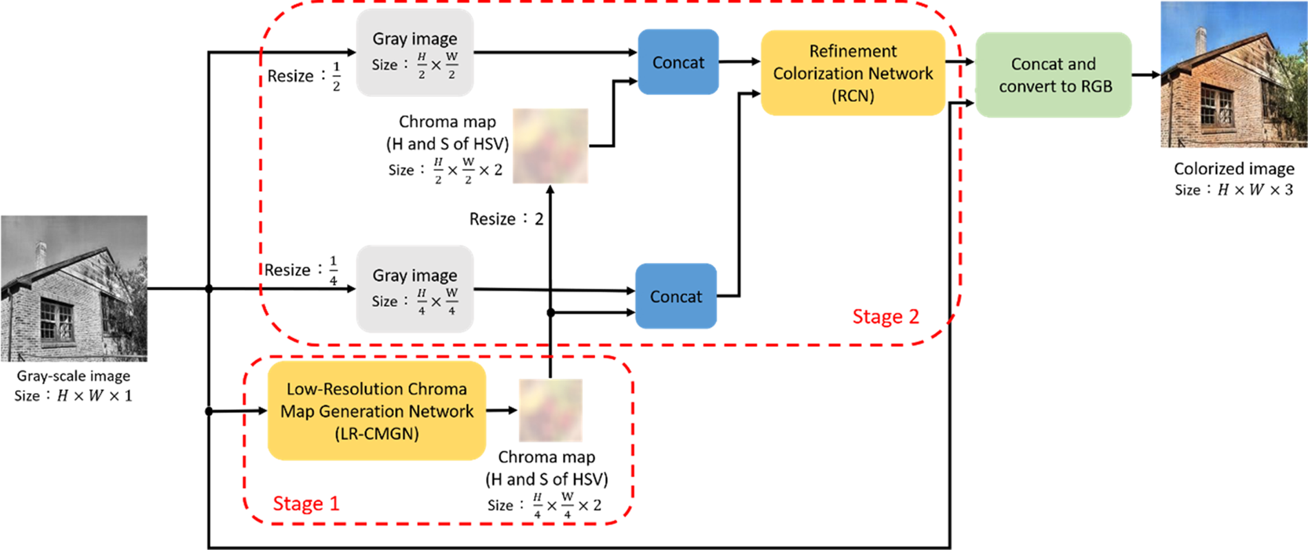
Fig. 1. Flowchart of proposed architecture.
A) Analysis of color spaces
[Reference Zhang, Isola and Efros25] explained the issue where the results of colorization using the Lab color space, despite being extensively utilized for modeling human perception such as [Reference Kinoshita, Kiya and Processing38], are tend to be low saturation. We believe that the definition of ab channels in Lab makes it hard to represent the saturation in a straightforward way because two parameters, a and b, are both involved with the saturation nonlinearly. As a consequence, during the training process, with existing loss functions, the difference in saturation between the prediction of model and ground truth is not easily minimized. The YUV color space is also a widely adopted color space in colorization tasks, but its chroma channels U and V have the same issue as the a and b parameters of the Lab color space.
We were inspired by this viewpoint and speculate that if neural networks can learn color saturation in a more informative way, this issue may resolve itself during the training process. We focused on the color spaces that enable saturation as an independent channel and investigated whether they can make the saturation of output images closer to the ground truth or not.
The HSV channel definition, where S stands for saturation, perfectly fits our needs. Furthermore, the HSV color space can match the human vision description more properly than Lab and YUV, allowing our model to learn in a more human-like manner and making the generated results more consistent with our perceptions. Taking into account all of the abovementioned factors, we selected HSV as our color space for training models to generate relevant chroma components.
B) Modeling
The way humans viewing images is to focus solely on either the whole or small parts of the image rather than on each pixel accuracy, making slight variations in pixel level, particularly in chroma components, difficult to detect. We conducted a basic experiment to confirm the practicality of this concept. We converted a set of randomly picked RGB images to the HSV color space and compared them to the images with low-resolution chroma maps. Figure 2(b) was created by downsizing the chroma maps of the original images in Fig. 2(a) to 1/4 size and then scaling up to the original size using bilinear interpolation. The results displayed in Fig. 2 show that, even if there might be some little artifacts in the image details when created from the low-resolution chroma maps, they can still reflect the majority of color information and the little artifacts will be removed later in our refining colorization network.

Fig. 2. Consequences of using low-resolution chroma maps. (a) Original images. (b) Images created using low-resolution chroma maps.
The above concept is incorporated in the design of the LR-CMGN to predict low-scale chroma maps with a size 1/16 of grayscale images. This design can lower the complexity of the whole model and make it easier to predict low-scale chroma maps correctly. This model consists of 12 layers of 3 × 3 convolutions, where all layers employ ReLU as the activation function except for the ${12^{\rm{th}}}$ layer, which uses tanh as the activation function, as shown in Fig. 3.

Fig. 3. Low-resolution chroma map generation network (LR-CMGN).
Although the low-resolution color map can represent the color of the whole image, there are still some differences from its ground truth, such as the stripes on the windows of the house and the car in Fig. 2. We proposed the RCN as a solution to this problem. The RCN architectural design is based on the image pyramid, and the performance of the model is enhanced by inputting and analyzing images of multiple scales, as shown in Fig. 4.
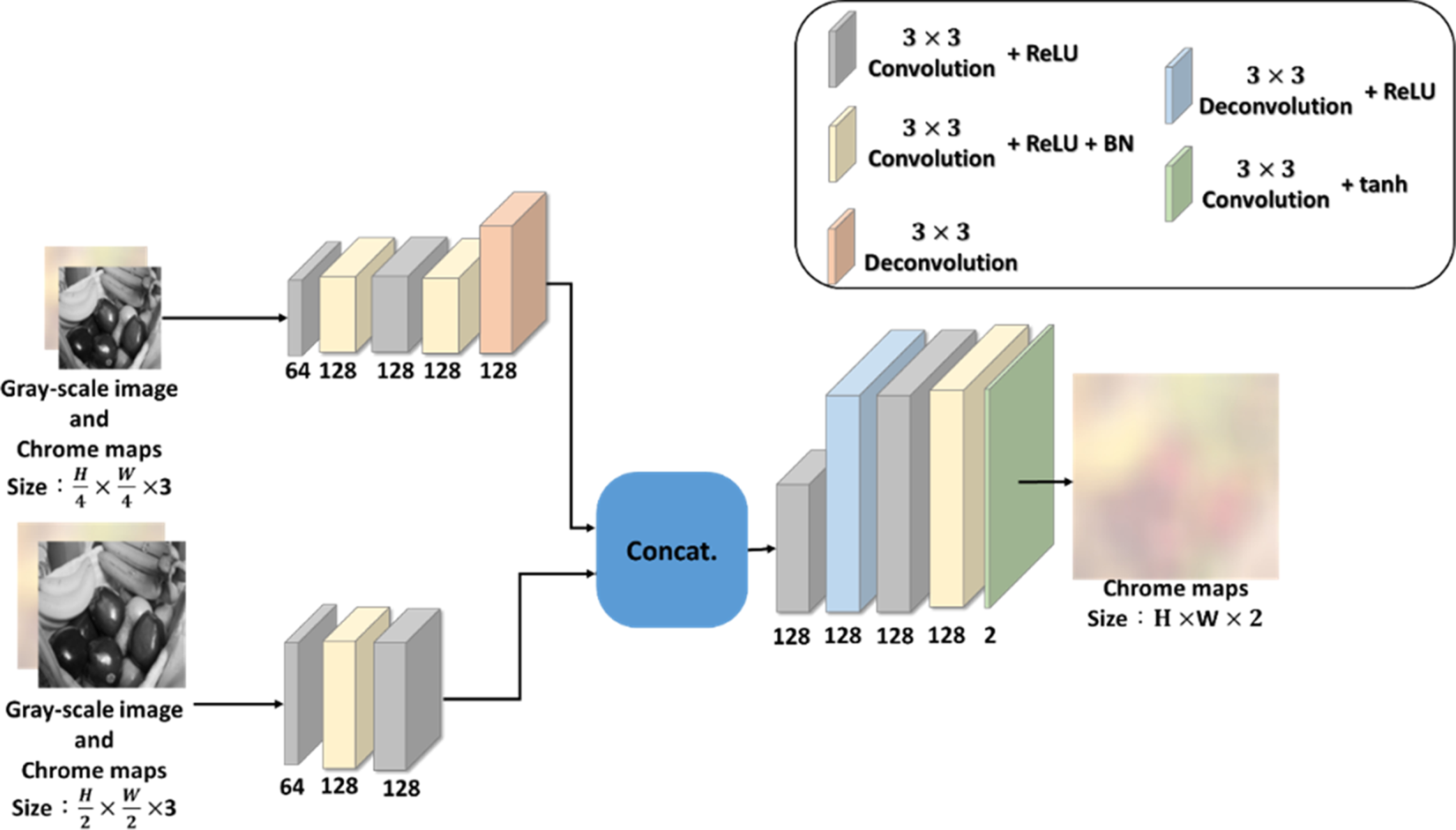
Fig. 4. Refinement colorization network (RCN).
We already know from the experiment in Fig. 2 that the chroma components in HSV color space are fine to be down-scaled due to the deficiency for humans to notice little changes in chroma channels at pixel level. Based on this assumption, our design differs from the existing pyramid structures in that they used more than two scales of information, whereas our method generates original-scale chroma maps from only low- and middle-scale information, allowing us to reduce the computational load of the model while still obtaining sufficient feature quality. Our implementation is more similar to [Reference Zhao, Shi, Qi, Wang and Jia37] than other works that used the pyramidal concept, in that we modified the last layer output of a network to obtain multi-scale features rather than collecting different scale features from the feed-forward process.
As shown in Fig. 4, our pyramidal RCN has two inputs with different scales, which are created by concatenating the output of the LR-CMGN with two different sizes of low-scaled grayscale images. We scale down the LR-CMGN output and the grayscale image using bilinear interpolation to 1/4 and 1/16 of the original grayscale image size. The low-scale and middle-scale features are extracted from their respective input images using two parallel convolutional sub-networks, and the output features representing two different scales are concatenated and fed into a de-convolutional layer to generate features of the same size as the original grayscale image. The H and S components of the HSV color space are predicted by analyzing these features, and the predicted results are combined with the grayscale image to form the colorized image.
C) Training details
Our colorization models were trained using the Places365-standard [Reference Zhou, Lapedriza, Khosla, Oliva and Torralba39] database, which contains 1.8 million training, 36 500 validation, and 320 000 test images covering 365 scene classes such as indoor scenery and urban scenery, with each scene containing a variety of objects such as humans, animals, and buildings that can help our models colorize diverse grayscale image contents. The training and validation sets were used to train the LR-CMGN and the RCN, and all images in the dataset have a resolution of 256 × 256 pixels.
We excluded grayscale images from the dataset to avoid the machine from learning incorrect information. To predict the H and S components of the HSV color space, the color space of the training images is converted from RGB to HSV, and the value ranges of all channels are normalized between −1 and 1. During training, the V and HS components are employed as input and ground truth, respectively.
Given the fact that the RCN input contains both the grayscale image and the LP-CMGN input, the output of LP-CMGN will affect the RCN prediction result. As a result, when training the colorization model, we first trained LP-CMGN to near-convergence, then trained the RCN while fine-tuning the LP-CMGN parameters at the same time. Since the LR-CMGN prediction is conducted in low-scale, which is 1/16 of original chroma maps, we utilized low-scale ground truth created by shrinking the ground truth using bilinear interpolation to train this network.
In our experiment, both subnetworks use the same loss function, as shown in (1), where ${S_{\rm{Loss}}}$ and ${H_{\rm{Loss}}}$
 represent the errors of S and H components predicted by the model, respectively, and these errors are calculated using the MAE (mean absolute error), and the weighting $\lambda$
 in the losses ${S_{\rm{Loss}}}$
 and ${H_{\rm{Loss}}}$
 is set to 1.

H is a color ring that represents color hue via angular dimension in the range [0°, 359°] and is normalized to [–1,1]. Since the color hue is specified in a circular ring and has dis-continuality at ${\pm} 1$ , there is a risk that the model will learn the incorrect color hue when using MAE to calculate the error. For instance, if the model predicts H to be −0.9, the loss should be minor if the ground truth H is 0.9, but the error computed by MAE between these two values is high and does not accurately represent the actual difference. To address this issue, we modified the MAE as (2), where p and g denote the outcome of model prediction and ground truth, respectively. As the fact that the difference between two angles of H components should never surpass 180°, or 1 after normalization. Thus, we design the loss function in (2) based on this principle. If the difference is more than 1, the output of the loss function must be adjusted; otherwise, the output remains intact. By applying our design loss function (2) to the above example, we can calculate the H loss accurately by changing the error from 1.8 to 0.2.

The Adam optimizer was used to train the model, which has the advantage of fast convergence, and the learning rate is set to 2 × 10⁻⁴ across 10 epochs. Since weight initialization has a substantial impact on the convergence speed and the performance of the model, the He initialization [Reference He, Zhang, Ren and Sun40] was employed to initialize the weights because it provides better training results of the model with the ReLU activation function than other techniques.
III. EXPERIMENTAL RESULTS
Our experiments were carried out using a PC with an Intel I7-4750 K at 4.00 GHz processor and an Nvidia GTX 1080 graphics card. Previous research in the literature has utilized the PSNR and the SSIM as objective image quality assessment metrics to evaluate the image quality of colorization, but since some objects might have multiple colors, and as [Reference Blau and Michaeli41] mentioned, these methods are unable to represent the true human perception, as illustrated in Fig. 5. Our result is clearly more natural than the other methods in Fig. 5, but our performance as measured by the PSNR and the SSIM is the lowest. As a result, we only subjectively assess the colorizing results.

Fig. 5. Problems in using objective image quality assessment metrics to evaluate colorization results. (a) Ground truth. (b) Iizuka et al. [Reference Iizuka, Simo-Serra and Ishikawa23]. (c) Zhang et al. [Reference Zhang, Isola and Efros25]. (d) Proposed method.
A) Comparisons of various model designs
To stress the necessity of our model architecture, we explain and compare the performance impact of our network components in this section. We initially investigate the differences in model outcomes with and without refinement network. We scale up the first-stage result by bilinear interpolation, and then concatenate the grayscale image to obtain the colorized image, as shown in Fig. 6(a).

Fig. 6. Images produced by colorization methods with different stages. (a) Only first-stage. (b) Proposed two-stage method.
Although these images are fairly close to natural images, they have blocky color distortion in some areas. In contrast, Fig. 6(b) shows the results of applying the refinement network restoration after the first-stage result. The restored results are more realistic than Fig. 6(a), and the refinement network is necessary as it overcomes the problem of blocky color artifacts.
Next, we discuss the structural design of the refinement network. Figure 7 depicts our initial refinement network architecture, which is not pyramidal and composed of 13 layers with 3 × 3 kernels, with no decreasing dimensionality of convolutional layers. The inputs are a grayscale image and scaled low-resolution chroma maps, and some results are shown in Fig. 8(a).
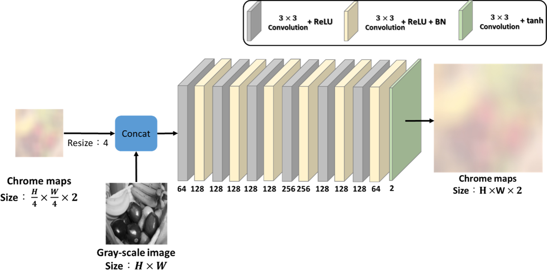
Fig. 7. Original design of refinement network.
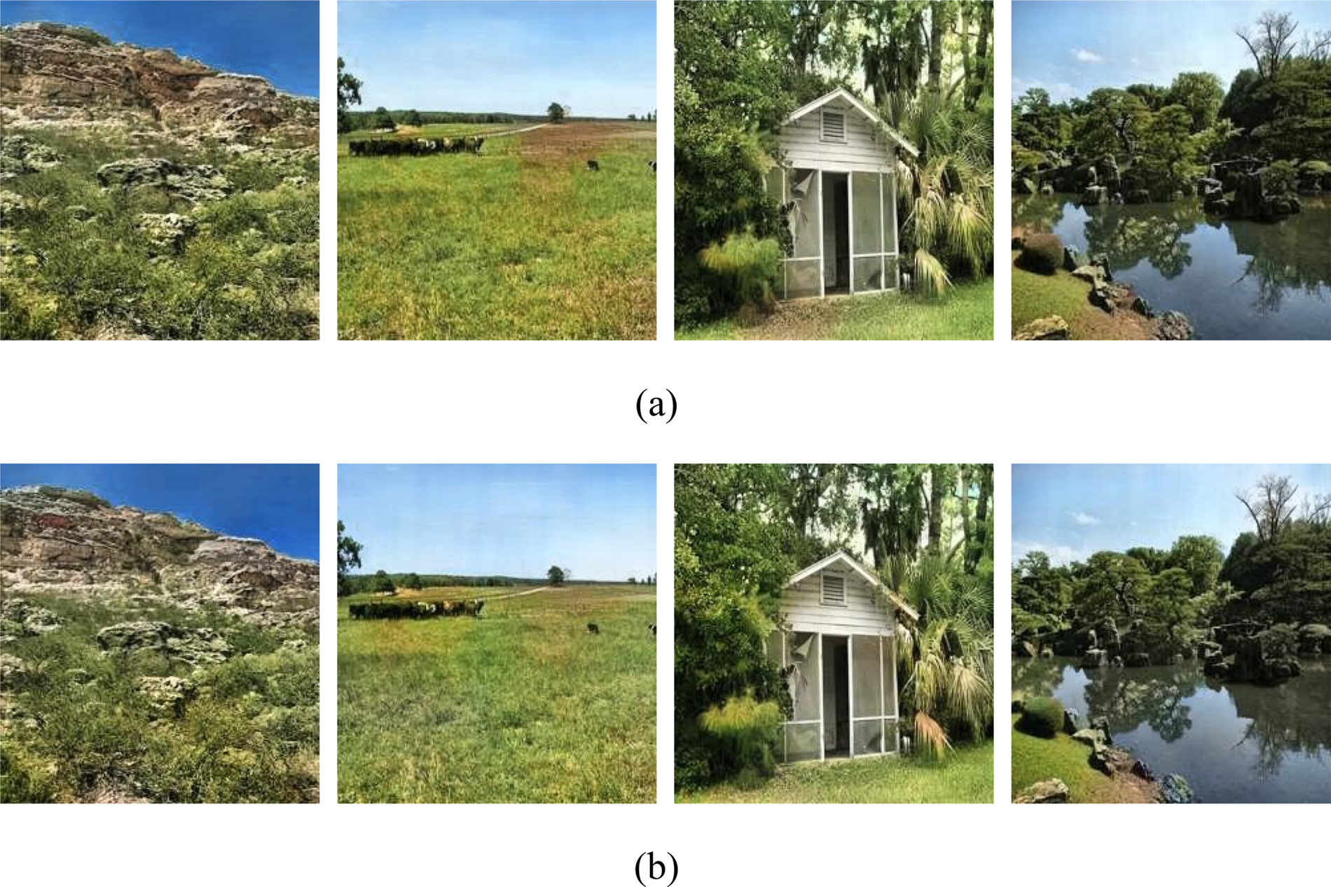
Fig. 8. Results of using different refinement network structures. (a) Original design (13 convolutional layers). (b) Pyramidal structure.
In comparison to our proposed pyramidal structure, which achieves very similar results, the parameters for the original design and pyramidal structure are 2.2 and 1.5 M, respectively. We can observe that the parameters of our pyramidal structure are only 0.68 times those of the original design, thus we use the pyramidal structure for our refinement network.
B) Comparisons of different color spaces
To demonstrate that HSV is a more suitable color space for colorization tasks, we compared the performance of the YUV, Lab, and HSV color spaces using the same network architecture and training conditions. We converted the training data into multiple color spaces and then used these training data to train the colorization models, resulting in different sets of parameters for each color space. Figure 9 compares and displays the colorized results of three models. We can notice that the HSV results are more realistic than the other color spaces, especially the higher saturation color on leaves, proving that HSV is the best choice.

Fig. 9. Comparisons of colorization results using different color spaces. (a) YUV. (b) Lab. (c) HSV.
C) Comparisons of different methods
We compare our proposed method with four popular or recent learning-based colorization methods [Reference Zhang8, Reference Iizuka, Simo-Serra and Ishikawa23, Reference Zhang, Isola and Efros25, Reference Vitoria, Raad and Ballester32]. Figures 10 and 11 show the results of these and our methods when colorizing indoor scenes and outdoor scenes, respectively. In comparison to the literature methods, our results for both scenes of images look more natural, have higher color saturation, and are closer to the ground truth. The color of colorized images created using the [Reference Iizuka, Simo-Serra and Ishikawa23] method is a bit dull, with more gray and brown. The results of [Reference Zhang, Isola and Efros25] have color bleeding artifacts in the indoor scene, such as the wall, floor, and garments, and in the outdoor scene, such as the chimney, roof. The colorized images by [Reference Zhang8] tend to have lower saturation than ours. The result of [Reference Vitoria, Raad and Ballester32] has colorization defects in texture parts, such as the chimney of the house and the bricks near the roof of the castle. More colorized images generated by our method are shown in Fig. 12.

Fig. 10. Comparisons of different colorization methods used on indoor images. (a) Ground truth. (b) [Reference Iizuka, Simo-Serra and Ishikawa23]. (c) [Reference Zhang, Isola and Efros25]. (d) [Reference Zhang8]. (e) [Reference Vitoria, Raad and Ballester32]. (f) Proposed method.

Fig. 11. Comparisons of different colorization methods used on outdoor images. (a) Ground truth. (b) [Reference Iizuka, Simo-Serra and Ishikawa23]. (c) [Reference Zhang, Isola and Efros25]. (d) [Reference Zhang8]. (e) [Reference Vitoria, Raad and Ballester32]. (f) Proposed method.

Fig. 12. More results by applying our method to grayscale images. (a) Grayscale image. (b) Ground truth. (c) Proposed method.
Table 1 shows the results of comparing the number of parameters of models. Comparing to others, our method uses a far smaller number of network parameters, while producing more realistic images.
Table 1. Comparisons of the number of models parameters.

D) Analysis of failure cases
Finally, we examine the failure cases of our method. We discover in the experiment that the ground truth images with much higher details than normal can sometimes cause colorization issues for our method. It is because that we begin by predicting the chroma channel at a lower scale, and it can be sometimes difficult to predict the appropriate chroma value when the targets are too small in size. This could lead to the failure in such places, such as the red-circled items in Fig. 13.

Fig. 13. Failure cases of our colorization method. (a) Ground truth. (b) Proposed method.
IV. CONCLUSION
In this research, we present a two-stage colorization model based on the CNN with a pyramidal structure that allows us to minimize our model parameters. To generate a colorized image, our method first generates low-scale chroma components by the LR-CMGN and then analyzes multi-scale information using the RCN. Our method addresses the issue that existing colorization methods tend to generate subdued and poor saturation results. We investigate how to create better colorized grayscale images using the HSV color space. To tackle the problem caused by the H component of the HSV color space represented by a color ring, we design a loss function that enables our model to predict the chroma components of HSV accurately. Our experiments with Places365-standard datasets validate that our outcomes are more natural and closer to the ground truth than previous methods.
Financial support
This work was partially supported by the Ministry of Science and Technology under the grant number MOST 110-2221-E-027-040-.
Conflict of interest
None.
Yu-Jen Wei received the B.S degree in the Department of Communication Engineering from the National Penghu University of Technology, Penghu, where he is currently pursuing the Ph.D. degree in electrical engineering from the National Taipei University of Technology, Taipei, Taiwan, R.O.C. He joined the Image and Video Processing Lab of the National Taipei University of Technology in 2016. His current research interests include image quality assessment, computer vision, and machine learning.
Tsu-Tsai Wei received the B.S. and M.S. degree in the Department of Electrical Engineering from the National Taipei University of Technology, Taipei, Taiwan, R.O.C in 2018 and 2021. He joined the Image and Video Processing Lab of the National Taipei University of Technology in 2017. His current research interests include convolution neural network and grayscale image colorization.
Tien-Ying Kuo received the B.S. degree from the National Taiwan University, Taiwan, R.O.C., in 1990 and the M.S. and Ph.D. degrees from the University of Southern California, Los Angeles, in 1995 and 1998, respectively, all in electrical engineering. In the summer of 1996, he worked as an intern in the Department of Speech and Image Processing, AT&T Laboratories, Murray Hill, NJ. In 1999, he was the Member of Technical Staff in the Digital Video Department, Sharp Laboratories of America, Huntington Beach, CA. Since August 2000, he has been an Assistant Professor and is currently an Associate Professor with the Department of Electrical Engineering, National Taipei University of Technology, Taipei, Taiwan, R.O.C. He received the best paper award from the IEEE International Conference on Intelligent Information Hiding and Multimedia Signal Processing (IIH-MSP) in 2008. His research interests are in the areas of digital signal and image processing, video coding, and multimedia technologies.
Po-Chyi Su was born in Taipei, Taiwan in 1973. He received the B.S. degree from the National Taiwan University, Taipei, Taiwan, in 1995 and the M.S. and Ph.D. degrees from the University of Southern California, Los Angeles, in 1998 and 2003, respectively, all in Electrical Engineering. He then joined Industrial Technology Research Institute, Hsinchu, Taiwan, as an engineer. Since August 2004, he has been with the Department of Computer Science and Information Engineering, National Central University, Taiwan. He is now a Professor and the Dept. Chair. His research interests include multimedia security, compression, and digital image/video processing.


 Open access