2. Experimental evidence of explicit and spontaneous symmetry breaking

Experiments were conducted using an annular combustor with 12 premixed flames operated at atmospheric conditions (see figure 1) and fuelled with a mixture of 70 % H$_2$ and 30 % CH$_4$ by power. The thermal power was fixed to 72 kW and the equivalence ratio was used as a bifurcation parameter. It was changed by adjusting the air mass flow, while keeping the fuel mass flow constant. It was varied between 0.4875 and 0.575 in steps of $1.25\times 10^{-2}$. The collected dataset which is used here to investigate the unexpected explicit rotational symmetry breaking of the thermoacoustic dynamics, is the same as the one used by Faure-Beaulieu et al. (Reference Faure-Beaulieu, Indlekofer, Dawson and Noiray2021a) to investigate the spontaneous reflectional symmetry breaking. The hydrogen–methane–air mixture is fed into a cylindrical plenum located at the bottom part of the combustor in figure 1(a). This plenum conditions and divides the flow into 12 axisymmetric burners. The burners are composed of 150 mm long tubes of 18.9 mm diameter, with central rods terminated by bluff bodies of 13 mm diameter. Just downstream of these bluff bodies, hot products recirculate, which ensures robust anchoring of the flames. In contrast to experiments by Worth & Dawson (Reference Worth and Dawson2013), the burner tubes are not equipped with a swirler, which is another typical element of gas turbine burners used to further strengthen the flame anchoring (Chterev et al. Reference Chterev2014). The burners are equally spaced around the circumference of the annular combustor, i.e. with 30$^{\circ }$ between each injector, as shown in the top view of the combustion chamber in figure 1(c). The inner and outer walls of the chamber were 120 and 300 mm long, respectively, with diameters of 127 and 212 mm. They were water cooled, enabling long run times and equilibrium wall temperatures.

Figure 1. (a) Model gas turbine combustor. (b) Phase-averaged flame chemiluminescence. (c) Acoustic pressure recorded with six transducers. During the selected interval, the thermoacoustic limit cycle is a quasi-purely spinning eigenmode.

Twelve Kulite (XCS-093-05D) pressure transducers were mounted at six azimuthal and two longitudinal positions flush with the inner wall of the burner tubes and recorded with a sampling rate of 51.2 kHz. The natural chemiluminescence of the flames viewed from the exhaust is recorded with a high speed camera using the same optical system as in the paper of Worth & Dawson (Reference Worth and Dawson2013). Figure 2(a) shows the averaged chemiluminescence, which can be considered as proportional to the heat-release rate in this perfectly premixed configuration, for a thermoacoustically stable operating point at $\varPhi =0.5$. Figure 2(b) depicts the time-averaged heat-release rate per burner for several operating conditions, showing small discrepancies between the flames with a standard deviation of approximately 5 %, although the burners are designed to be identical and the cylindrical plenum to be axisymmetric. For each $\varPhi$, the combustor was ignited, run for at least 60 s to reach thermal equilibrium before recording 100 s of acoustic data while keeping the operating condition constant, and then turned off. The sound pressure level (SPL) in the annular combustor is plotted in figure 3(a) for four $\varPhi$. When $\varPhi =0.5$, the thermoacoustic system is linearly stable. The strongest resonance corresponds to an eigenmode whose azimuthal distribution exhibits one acoustic wavelength along the annular chamber circumference, and whose frequency is approximately 1090 Hz. The resonance oscillation of the different modes is sustained by the inherent broadband acoustic forcing from the turbulent combustion process. For larger $\varPhi$, the acoustic energy production resulting from the constructive thermoacoustic feedback exceeds the acoustic energy dissipation, and the dominant eigenmode becomes linearly unstable. Under these conditions, thermoacoustic limit cycles are reached at the aforementioned resonance frequency (Noiray & Schuermans Reference Noiray and Schuermans2013a). Their dynamics is governed by the nonlinear coherent response of the flame to the acoustic field and by the turbulent fluctuations of the heat-release rate.

Figure 2. (a) Averaged overhead heat-release rate for $\varPhi =0.5$. (b) Heat release rate per burner normalized by the average heat-release rate.

Figure 3. (a) SPL for increasing $\varPhi$. (b) Selected intervals for $\varPhi =0.55$, during which the azimuthal mode is mixed, with CW and CCW spinning directions. The angles in the legend correspond to the locations of the transducers.

Figure 3(b) presents the acoustic pressure $p$ at three azimuthal locations during two short intervals (I) and (II) of the 100 s record for $\varPhi =0.55$, for which the self-sustained azimuthal thermoacoustic mode spins in the CCW and in the CW direction.

Recently, Ghirardo & Bothien (Reference Ghirardo and Bothien2018) proposed a new ansatz for the acoustic pressure field based on quaternions to describe azimuthal eigenmodes in annular combustors. A set of four state variables $A, \theta, \chi$ and $\varphi$, which vary slowly with respect to the fast acoustic time scale $2{\rm \pi} /\omega$, and which can be extracted from the acoustic pressure time series, allows the following well-defined description of the state of an azimuthal thermoacoustic mode:

(2.1)\begin{equation} \tilde{p}(\varTheta,t)=A(t)\,{\rm e}^{i(\theta(t)-\varTheta)}\,{\rm e}^{{-}k\chi(t)}\,{\rm e}^{j (\omega{t}+\varphi(t))},\end{equation}

where $t$ and $\varTheta$ are the time and the azimuthal coordinate, and $i$, $j$ and $k$ are the quaternion units. The acoustic pressure is $\text {Re}(\tilde {p})$. It can be expanded as

(2.2)\begin{equation} p(\varTheta,t)=A\cos(\varTheta-\theta)\cos(\chi)\cos (\omega{t}+\varphi)+ A\sin(\varTheta-\theta)\sin (\chi)\sin(\omega{t}+\varphi),\end{equation}

and $A$ is the real-valued positive slowly varying amplitude. The slowly varying angle $\theta$ describes the position of the anti-nodal line and the eigenmode state is identical for $\theta$ and $\theta +{\rm \pi}$. The slowly varying angle $\chi$ indicates whether the azimuthal eigenmode is a standing wave ($\chi =0$), a pure CW or CCW spinning wave ($\chi =\mp {\rm \pi}/4$) or a mix of both for $0<|\chi |<{\rm \pi} /4$. The angle $\varphi$ stands for slow temporal phase drift. These variables fully describe the acoustic fields $p$ as a function of the time and azimuthal position.

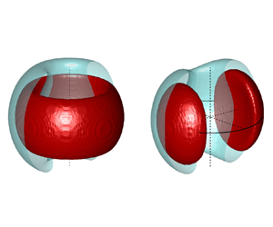
Figure 4(a) shows the time traces of the extracted slow-flow variables together with their probability density functions (PDFs) for the last 6 s of the record, an interval that is representative of the stationary dynamics when $\varPhi =0.55$. The joint PDF of the first three state variables deduced from the 100 s record at $\varPhi =0.55$ is also shown in figure 5(b), where $A$, $\theta$ and $2\chi$ are taken as spherical coordinates as shown in figure 5(a).

Figure 4. (a) Evolution of slow-flow variables that define the state of the azimuthal thermoacoustic mode, during the last 6 s of the experimental record for $\varPhi =0.55$, together with their PDFs. (b) PDFs and time traces from the time-domain simulations of (6.5), which includes both resistive and reactive asymmetries ($\varepsilon =0.0023$, $\varTheta _\varepsilon =0.66$ rad, $\varGamma /\omega ^{2}=4.2\times 10^{5}$ Pa$^{2}$ s$^{-1}$, $\nu =17$ s$^{-1}$, $c_2\beta =17$ s$^{-1}$, $\varTheta _\beta =0.63$ rad and $\kappa =1.2\times 10^{-4}\ \text {Pa}^{-2}\ \text {s}^{-1}$).

Figure 5. (a) Bloch sphere representation of the state of the azimuthal mode. (b,c) Experimental joint PDFs for $\varPhi =0.525, 0.55$.

At the condition $\varPhi =0.55$, the amplitude of the azimuthal mode has a relatively small standard deviation compared with its mean value. The intermittent changes of sign of the nature angle $\chi$ correspond to changes of spinning direction of the mixed mode, as shown in figure 3(b). Although the difference is small, the most probable orientation of the anti-nodal line of the mixed mode's standing component is not the same whether the mode spins CW or CCW, a phenomenon that had never been reported and that will be explained at the end of the paper.

We now consider the evolution of the state variable PDFs in the vicinity of the Hopf bifurcation. These stationary PDFs are shown in the left column of figure 6 for several values of the bifurcation parameter $\varPhi$. Also, the time evolution of these state variables during 6 s intervals at four of the stationary operating conditions are presented in figure 7.

Figure 6. Stationary PDFs of $A$, $\chi$, $\theta$ and $\varphi$ at several $\varPhi$ in the vicinity of the supercritical Hopf bifurcation. The PDFs are deduced from the slow-flow variable time traces, which are extracted from the acoustic pressure time traces following the procedure in Ghirardo & Bothien (Reference Ghirardo and Bothien2018). For (a)–(d), the acoustic time traces were obtained experimentally. For (e–h), the acoustic time traces were obtained by simulating 100 s of (3.1). Linear dependencies with respect to $\varPhi$ of the parameters ($\nu$, $c_2\beta$, $\kappa$, $\varGamma$) were deduced from the data processing and presented in figure 9. For the simulations, $\varTheta _\beta$ has simply been kept at a constant value of 0.63 rad, which corresponds to the average value of $\theta$ observed in the experiments. The spontaneous reflectional symmetry breaking of the thermoacoustic dynamics, i.e. a clearly preferred spinning direction, is seen in the PDF of $\chi$ and occurs when $\varPhi$ is increased from from 0.5625 to 0.575. The explicit rotational symmetry breaking of the thermoacoustic dynamics, i.e. a clearly preferred nodal line orientation, manifests itself in the PDF of $\theta$ and is visible for the entire range of $\varPhi$.

Figure 7. Experimental time traces of the state variables under stationary operating condition for different equivalence ratios. The duration of these time traces (6 s) is the same as the one presented in figure 2(c) of the main document. The extraction of the instantaneous state variables $A$, $\chi$, $\theta$ and $\varphi$ from the acoustic pressure signals is performed using the method proposed in Ghirardo & Bothien (Reference Ghirardo and Bothien2018).

The evolution of $P(A)$, shown in figure 6(a), is typical of a supercritical Hopf bifurcation in presence of additive random forcing (Juel, Darbyshire & Mullin Reference Juel, Darbyshire and Mullin1997). The bifurcation occurs around $\varPhi =0.5125$. This point separates broadband-noise-driven resonances, when the azimuthal thermoacoustic mode is linearly stable, from limit cycles, when it is linearly unstable. The change of the mean amplitude is relatively smooth, which allows us to exclude the possibility of a sub-critical Hopf bifurcation, such as the ones investigated by Gopalakrishnan et al. (Reference Gopalakrishnan, Tony, Sreelekha and Sujith2016) or Noiray (Reference Noiray2017). Next, one can consider how $P(\varphi )$ changes with $\varPhi$ in figure 6(d). Overall, the slowly varying temporal phase $\varphi$ drifts sufficiently during these 100 s records to yield rather flat distribution between 0 and $2{\rm \pi}$. One can notice that some phases are statistically prevailing for the higher range of investigated $\varPhi$, but these PDF maxima differ from case to case, and moreover, they wane when longer time traces are considered for computing the statistics, in agreement with the model which we propose in this article.

More interesting are the statistics of $\theta$ and $\chi$, which are respectively associated with an explicit rotational symmetry breaking and with a spontaneous reflectional symmetry breaking of the thermoacoustic dynamics in this work. Let us begin with $P(\theta )$ in figure 6(c): even though the combustor was designed as rotationally symmetric as possible with a discrete rotational symmetry of order 12 (due to the 12 burners), the experimental results show a clearly preferred and repeatable anti-nodal line position for the different $\varPhi$. Given the long run times and the high-order discrete rotational symmetry of the chamber, one would either expect a quasi-uniform distribution of $\theta$ or a new preferred nodal line direction each time the combustor is ignited. The only explanation for the repeatable preferred orientation is the presence of an explicit rotational symmetry breaking in the thermoacoustic system.

In addition to this explicit rotational symmetry breaking, the thermoacoustic dynamics exhibits a spontaneous reflectional symmetry breaking, which has been investigated by Faure-Beaulieu et al. (Reference Faure-Beaulieu, Indlekofer, Dawson and Noiray2021a) and which manifests itself in figure 6(b): When $\varPhi <0.55$, $P(\chi )$ is unimodal, with a maximum close to zero, indicating that the thermoacoustic mode is mixed, with predominant standing wave component, which corroborates the theoretical studies from Faure-Beaulieu & Noiray (Reference Faure-Beaulieu and Noiray2020) and Ghirardo & Gant (Reference Ghirardo and Gant2021). Considering figure 7, one can see that the underlying time traces exhibit erratic fluctuations of $\chi$ around 0. For $0.55\leq \varPhi \leq 0.5625$, $P(\chi )$ is bimodal, which indicates that the spinning wave component of the mixed mode is predominant. The intermittent changes of spinning direction for $\varPhi =0.55$, shown in figures 4(a) and 7, are less frequent and more pronounced than for $\varPhi =0.525$. When the equivalence ratio is further increased to $\varPhi =0.575$, one can see in figure 6(b) that the sporadic reversals of spinning direction do not take place anymore: the mixed mode spins in the CW direction and the symmetry of its state PDF is spontaneously broken beyond this threshold. As explained by Faure-Beaulieu et al. (Reference Faure-Beaulieu, Indlekofer, Dawson and Noiray2021a), this spontaneous reflectional symmetry breaking is due to the fact that the intensity of the inherent stochastic forcing is too low to induce further crossing of the potential barrier separating the CW and the CCW attractors. It is worth noting that, when the combustor is ignited and ramped up to $\varPhi =0.575$, the final stationary thermoacoustic state can also be the CCW mixed mode, which is shown in figure 8, and which demonstrates that both attractors coexist. The model presented in the remainder of this article, reproduces both the reflectional spontaneous symmetry breaking and the unexpected rotational explicit symmetry breaking.

Figure 8. Experimental time traces of the state variables at $\varPhi =0.575$ a thermal power of 72 kW. Two independent tests were performed. For each of them, the annular combustor is ignited and set to the same operating condition $\varPhi =0.575$. The twenty seconds time traces of $\chi$ show that the final steady state can either be a CW mixed mode or a CCW one.

3. Thermoacoustic wave equation

In the work of Faure-Beaulieu & Noiray (Reference Faure-Beaulieu and Noiray2020), the quaternion acoustic field was inserted into the following wave equation with distributed heat-release rate fluctuations to model the thermoacoustic dynamics of an idealized thin annular chamber:

(3.1)\begin{equation} \frac{\partial^{2} p}{\partial t^{2}} + \alpha \frac{\partial p}{\partial t} - \frac{c^{2}}{\mathcal{R}^{2}} \frac{\partial^{2} p}{\partial \varTheta^{2}} = (\gamma - 1)\:\frac{\partial \dot{Q}}{\partial t} + \varXi(\varTheta,t). \end{equation}

In this equation, $\alpha$ is the acoustic damping at the annulus boundaries, $\mathcal {R}$ the annulus radius, $c$ the speed of sound, $\gamma$ the heat capacity ratio, $\dot {Q}(\varTheta,t)$ the coherent component of the heat-release-rate fluctuations and $\varXi$ a spatially distributed white Gaussian noise representing the effect of turbulent fluctuations of the heat-release rate (e.g. Clavin, Kim & Williams Reference Clavin, Kim and Williams1994; Lieuwen Reference Lieuwen2003; Lieuwen & Banaszuk Reference Lieuwen and Banaszuk2005; Noiray & Schuermans Reference Noiray and Schuermans2013a). The coherent heat-release-rate fluctuations are then linked to the acoustic field using the expression

(3.2)\begin{equation} (\gamma-1)\dot{Q}=\beta [1+c_2\cos(2(\varTheta-\varTheta_{\beta})] p -\kappa p^{3}. \end{equation}

The first term stands for the linear response of the fluctuating heat-release rate to acoustic perturbations. If $\beta >\alpha$ and $c_2=0$, the linear growth rate of the thermoacoustic mode $\nu =(\beta -\alpha )/2$ is positive, i.e. the mode is linearly unstable, and small acoustic perturbations are exponentially amplified. This pure exponential growth is not observed in real combustors because of the inherent turbulence-induced stochastic forcing $\varXi$ and because of the nonlinearity of the flame response to the acoustic field beyond a certain level. The first term also accounts for spatial non-uniformities along the annulus, through the second component $c_2 \cos (2(\varTheta -\varTheta _{\beta }))$ of the Fourier series of any distribution of heat-release-rate source, which is the only component influencing the first azimuthal eigenmode as shown by Noiray et al. (Reference Noiray, Bothien and Schuermans2011). Given that real nominally symmetric combustors always exhibit some small asymmetries – this fact is exemplified by the mean heat-release-rate distribution of the present experimental system shown in figure 2 – it is crucial to use this Fourier series in the model, because it will be shown that even imperceptible non-uniformities of the thermoacoustic coupling have a significant observable effect close to the bifurcation. The angle $\varTheta _{\beta }$ is the direction of maximum root mean square acoustic pressure. In the theoretical studies of Noiray et al. (Reference Noiray, Bothien and Schuermans2011) and Faure-Beaulieu & Noiray (Reference Faure-Beaulieu and Noiray2020), the assumption $\varTheta _{\beta }=0$ was made for simplicity, and without loss of generality, because the origin of $\varTheta$ can be chosen arbitrarily. In the present work, we keep the same origin for all the operating points because the preferential orientation of the mode can vary for different operating conditions. The second term of (3.2), $-\kappa p^{3}$, defines the saturation of flame response, which leads to limit cycle oscillations, and is sufficient to adequately capture the thermoacoustic dynamics in the vicinity of supercritical Hopf bifurcations as in the works from Lieuwen (Reference Lieuwen2003), Noiray & Denisov (Reference Noiray and Denisov2017), Hummel et al. (Reference Hummel, Berger, Stadlmair, Schuermans and Sattelmayer2018) and Lee et al. (Reference Lee, Kim, Gupta and Li2021). Possible non-uniformities of the nonlinear term are not accounted for in order to ease the parameter identification process. The modelling assumptions are now discussed in more detail.

First, real annular combustors have an overall toroidal shape but they also include complex three-dimensional (3-D) geometrical features. Consequently, their acoustic field can only be predicted using the 3-D wave equation. However, in the present paper, we are only interested by the azimuthal distribution of the acoustic modes at fixed radial and axial positions. Therefore, we can describe the dynamics of this azimuthal component with a one-dimensional (1-D) wave equation (e.g. Noiray & Schuermans Reference Noiray and Schuermans2013b; Faure-Beaulieu & Noiray Reference Faure-Beaulieu and Noiray2020; Faure-Beaulieu et al. Reference Faure-Beaulieu, Indlekofer, Dawson and Noiray2021b).

Then, the saturation of the flame response to acoustic perturbations is simply modelled as $\dot {Q}=\beta p-\kappa p^{3}$, or $\dot {Q}=\beta p(1+c_2\cos (2(\varTheta -\varTheta _{\beta })))-\kappa p^{3}$ in presence of second-order asymmetry in the linear thermoacoustic coupling term. This low-order model, with linear and cubic term only, is a valid description in the vicinity of a supercritical Hopf bifurcation. Higher-order polynomials or sigmoid-type functions could be used to extend its validity further away from the Hopf point (Noiray Reference Noiray2017; Bonciolini et al. Reference Bonciolini, Faure Beaulieu, Bourquard and Noiray2021; Lee et al. Reference Lee, Kim, Gupta and Li2021). However, using a more elaborate nonlinear flame response model complicates the parameter identification. Considering that in this article, we focus on the neighbourhood of the Hopf point, we use the simple cubic nonlinearity, which corresponds to the normal form of the bifurcation.

Furthermore, considering that, in practice, coherent heat-release-rate oscillations resulting from acoustic perturbations occur after a certain convective delay, it may seem inappropriate to omit this phase lag in the model for $\dot Q$. Indeed, acoustic pressure fluctuations in the combustion chamber and in the plenum induce coherent velocity and equivalence ratio perturbations in the burners which do not instantaneously propagate to the flame, i.e. there is a phase lag between the acoustic field and the coherent heat-release-rate response. A model with such phase lag was derived by Faure-Beaulieu & Noiray (Reference Faure-Beaulieu and Noiray2020) but it is not used in this paper for the following reasons: firstly, accounting for a convective delay in this model does not substantially change the phase space topology when it is short compared with the inverse of the thermoacoustic growth rates, which is usually true in practice. The interested reader can refer to the work by Bonciolini et al. (Reference Bonciolini, Faure Beaulieu, Bourquard and Noiray2021) where the validity of this simplification for low-order modelling of thermoacoustic instabilities is discussed in detail. Secondly, accounting for it would necessitate the identification of an additional parameter (the time delay), which cannot be achieved in a robust manner with the observables (acoustic pressure signals at six azimuthal locations in the annular combustor) considered in the present work.

Next, it is worth mentioning that a nonlinear flame response model, which depends not only on the acoustic pressure load across the burners but also on the azimuthal acoustic velocity in the annular chamber, has also been proposed by Ghirardo & Juniper (Reference Ghirardo and Juniper2013). In that paper, a deterministic analysis shows that, with such a flame response model, standing modes can be attractors even in the absence of asymmetry. In that scenario, the nodal line direction is solely defined by the initial condition. This means that, in practice, it would stabilize at a random value after each ignition of the combustor. It would thus not exhibit a statistically prevailing direction, which is indisputably an evidence of spatial asymmetry in the configuration, and which we observe in the present work. The theoretical work of Ghirardo & Juniper (Reference Ghirardo and Juniper2013) followed, and inspired experimental and theoretical studies (e.g. O'Connor & Lieuwen Reference O'Connor and Lieuwen2011; Acharya et al. Reference Acharya, Aguilar, Malanosk and Lieuwen2014; Saurabh & Paschereit Reference Saurabh and Paschereit2017; Smith et al. Reference Smith, Emerson, Proscia and Lieuwen2018; Li et al. Reference Li, Yang, Li and Zhu2019) where combinations of axial and transverse acoustic forcing of compact swirled turbulent flames were considered. Besides, it can be noted that, in the work of Berger et al. (Reference Berger, Hummel, Hertweck, Kaufmann, Schuermans and Sattelmayer2017) and of Hummel et al. (Reference Hummel, Berger, Hertweck, Schuermans and Sattelmayer2017), the response of a non-compact swirled flame to transverse acoustic excitation was investigated for the case of high frequency thermoacoustic instabilities. However, since a simple model, which only involves the acoustic pressure load across the burners, allows us to satisfactorily reproduce and explain the main experimental observations, we do not include the additional possible effect of the azimuthal acoustic velocity in our flame response model.

Another relevant mechanism that is not considered in our model is the effect of the mean azimuthal flow on the thermoacoustic coupling, which was recently investigated by Bauerheim, Cazalens & Poinsot (Reference Bauerheim, Cazalens and Poinsot2015) and Faure-Beaulieu & Noiray (Reference Faure-Beaulieu and Noiray2020). Indeed, it is predicted in § IX of Faure-Beaulieu & Noiray (Reference Faure-Beaulieu and Noiray2020) that, for an idealized combustor with heat-release rate occurring in a region with a net azimuthal flow, the spinning mode rotating against the azimuthal mean flow direction attracts the dynamical system with more strength than the co-rotating spinning mode. This mechanism could be a possible explanation for very recent experimental observations by Ghirardo et al. (Reference Ghirardo, Nygård, Cuquel and Worth2021). In the latter work, the authors used a combustor with the same architecture and main dimensions as in the present paper. However, they had more burner tubes (18 instead of 12) and these burners were equipped with axial swirlers. Consequently, the reactive flow field in the combustor substantially differed from the one studied in this work. In particular, one can see in figure 2 of Ghirardo et al. (Reference Ghirardo, Nygård, Cuquel and Worth2021), that the mean heat-release rate is concentrated toward the inner radius of the annular combustion chamber, where the co-rotating swirling flames, uniformly distributed along the annulus, impart a CW swirling motion to the flow. On the other hand, towards the outer radius, there is a bulk swirling motion in the CCW direction, as it was sketched with black arrows in figure 1(c) of Worth & Dawson (Reference Worth and Dawson2014). Assuming that the coherent fluctuating heat-release rate is more intense toward the inner wall of the chamber, where the mean heat-release rate is larger and where the flow exhibits a substantial bulk azimuthal velocity in the CW direction, the theory proposed in § IX of Faure-Beaulieu & Noiray (Reference Faure-Beaulieu and Noiray2020) could be an explanation for the reported predominance of the CCW spinning thermoacoustic mode with this particular combustor. One can also note that these observations are in agreement with the forced experiments reported by Nygård et al. (Reference Nygård, Mazur, Dawson and Worth2019). Now, considering that in the present work, the burner tubes do not have swirlers, it can be assumed that the hot product velocity in the annulus does not exhibit an azimuthal component. Therefore, this feature of the model from Faure-Beaulieu & Noiray (Reference Faure-Beaulieu and Noiray2020) is not included in this work.

The parameters of the model given by (3.1) and (3.2) can be identified from the experimental data. To that end, we do not use the acoustic pressure time traces directly. Instead, we consider the time evolution of the state variables $A$, $\theta$, $\chi$ and $\varphi$, which can be extracted from the acoustic pressure traces, in order to achieve a robust model-based and data-driven parameter identification. In fact, this method necessitates a time-domain model for the state variables, which is presented in § 4. Once identified, the parameters will be used to perform time-domain simulations of (3.1) in § 5.

4. Langevin equation for the state variables

The coupled Langevin equations for $A$, $\theta$, $\chi$ and $\varphi$, derived by Faure-Beaulieu & Noiray (Reference Faure-Beaulieu and Noiray2020) by performing spatial and temporal averaging of (3.1), are very convenient to perform parameter identification, because they allow us to separate the contribution of the different parameters in distinct equations and therefore to reliably identify them. This system of equation is written as

(4.1)\begin{equation} \dot{\boldsymbol{Y}} = \boldsymbol{F}(\boldsymbol{Y}) + \boldsymbol{\mathsf{B}}(\boldsymbol{Y}) \boldsymbol{N},\end{equation}

and governs the dynamics of the azimuthal mode state vector $\boldsymbol {Y}=(A,\chi,\theta,\varphi )^{T}$ via a deterministic contribution $\boldsymbol {F}(\boldsymbol {Y})$ and a stochastic forcing term $\boldsymbol{\mathsf{B}}(\boldsymbol {Y}) \boldsymbol {N}$, where $\boldsymbol {N}=(\zeta _A, \zeta _\chi, \zeta _\theta, \zeta _\varphi )^{T}$ is a vector of independent white Gaussian noises of intensity $\varGamma /2\omega ^{2}$. The latter intensity involves the constant $\varGamma$, which is the spatially averaged stochastic forcing level originating from the turbulent fluctuations of the heat-release rate. The expressions for $\boldsymbol {F}$ and $\boldsymbol{\mathsf{B}}$ were derived by Faure-Beaulieu & Noiray (Reference Faure-Beaulieu and Noiray2020) and are given below

(4.2)\begin{gather} F_A(\boldsymbol{Y})=\left(\nu + \frac{c_{2}\beta}{4}\cos(2(\theta-\varTheta_{\beta})) \cos(2\chi)\right)A -\frac{3\kappa}{64}(5+\cos(4\chi))A^{3} + \frac{3{\varGamma}}{4\omega^{2}A}, \end{gather}

(4.3)\begin{gather}F_\chi(\boldsymbol{Y})=\frac{3\kappa}{64}A^{2}\sin(4\chi) -\frac{c_{2}\beta}{4}\cos(2(\theta-\varTheta_{\beta})) \sin(2\chi) - \frac{\varGamma\tan(2\chi)}{2\omega^{2}A^{2}}, \end{gather}

(4.4)\begin{gather}F_\theta(\boldsymbol{Y})={-}\frac{c_{2}\beta}{4} \frac{\sin(2(\theta-\varTheta_{\beta}))}{\cos(2\chi)}, \end{gather}

(4.5)\begin{gather}F_\varphi(\boldsymbol{Y})=\frac{c_2\beta}{4}\sin (2(\theta-\varTheta_{\beta}))\tan(2\chi), \end{gather}

where we introduced $\nu = (\beta -\alpha )/2$, which is the linear growth rate of the amplitude $A$ in absence of asymmetries ($c_2=0$), and where

(4.6)\begin{equation} \boldsymbol{\mathsf{B}}(\boldsymbol{Y})= \left(\begin{array}{cccc}1 & 0 & 0 & 0 \\0 & A^{{-}1} & 0 & 0 \\ 0 & 0 & (A\cos(2\chi))^{{-}1} & 0 \\0 & 0 & -\tan(2\chi)/A & A^{{-}1}\end{array}\right). \end{equation}

The analysis of the equilibrium points of $\boldsymbol {\dot {Y}} = \boldsymbol {F}(\boldsymbol {Y})$ was performed in Faure-Beaulieu & Noiray (Reference Faure-Beaulieu and Noiray2020), where it was shown that, for an ideal axisymmetric geometry with $c_2=0$ and $\varGamma \neq 0$, the attractor of the deterministic part of (4.1) is a mixed mode when $27\kappa \varGamma /(256\nu ^{2}\omega ^{2})<1$ or otherwise a standing mode. In both cases, the instantaneous anti-nodal line $\theta$ drifts slowly according to a random walk. For annular chambers featuring a certain degree of azimuthal asymmetry but without stochastic forcing ($c_2\neq 0$ and $\varGamma = 0$), the attractors are mixed modes if $c_2\beta /(2\nu )<1$ and otherwise standing modes, which was already found in Noiray et al. (Reference Noiray, Bothien and Schuermans2011).

This model cannot be used to predict the stability and slow-flow dynamics of a real combustor from the knowledge of its geometry and operating condition. However, as mentioned above, we show here that its handful of parameters $[\nu ; c_2\beta ; \kappa ; \varGamma ]$ can be identified from the experimental data and then the model can reproduce the thermoacoustic dynamics.

Several methods are available for disentangling deterministic and stochastic contributions in stochastic trajectories (e.g. Brückner, Ronceray & Broedersz Reference Brückner, Ronceray and Broedersz2020; Ferretti et al. Reference Ferretti, Chardès, Mora, Walczak and Giardina2020; Frishman & Ronceray Reference Frishman and Ronceray2020). Here, we use a method, which was adapted from the work of Friedrich and co-workers (Siegert, Friedrich & Peinke Reference Siegert, Friedrich and Peinke1998; Friedrich et al. Reference Friedrich, Renner, Siefert and Peinke2002; Böttcher et al. Reference Böttcher, Peinke, Kleinhans, Friedrich, Lind and Haases2006; Friedrich et al. Reference Friedrich, Peinke, Sahimi and Reza Rahimi Tabar2011) to the investigation of nonlinear oscillators subject to random forcing (e.g. Noiray & Schuermans Reference Noiray and Schuermans2013a; Bonciolini, Boujo & Noiray Reference Bonciolini, Boujo and Noiray2017; Boujo & Noiray Reference Boujo and Noiray2017; Noiray & Denisov Reference Noiray and Denisov2017; Boujo et al. Reference Boujo, Bourquard, Xiong and Noiray2020), and which was applied to thermoacoustic and aeroacoustic instabilities. More recently, this framework was further developed and used for the analysis of global hydrodynamic instabilities in turbulent flows (e.g. Lee et al. Reference Lee, Zhu, Li and Gupta2019; Callaham et al. Reference Callaham, Loiseau, Rigas and Brunton2021; Sieber, Paschereit & Oberleithner Reference Sieber, Paschereit and Oberleithner2021).

First, for each $\varPhi$, the transition probabilities of the state variables are extracted. Then, these probabilities are used to compute the first and second Kramers–Moyal coefficients that serve as basis for parameter identification with least square fitting. More details about the robustness of the parameter identification are given in the Appendix A of this article. The results of this model-based data-driven parameter identification are presented in figure 9. It was found that simple linear regression for the dependencies of $\nu =(\beta -\alpha )/2$, $c_2\beta$, $\kappa$ and $\varGamma$ on $\varPhi$ allows to unravel the complex topology of the phase space. Indeed, in § 5, these parameters are used to run time-domain simulations of the wave equation (3.1) to generate 100 s acoustic time series for each $\varPhi$, from which the state variables and their statistics are extracted and successfully compared with the ones of the experiments.

Figure 9. Parameters identified with the model-based data-driven approach explained in the Appendix A. The identified value for $\kappa$ is $1.2\times 10^{-4}\ \text {Pa}^{-2}\ \text {s}^{-1}$. Continuous lines show the linear regressions of the model parameters as a function of $\varPhi$.

5. Time-domain simulations of the thermoacoustic dynamics

For each of the values of $\varPhi$ considered in the experiments, a time-domain simulation of the thermoacoustic problem given by (3.1) and (3.2) is performed with the identified linear functions of $\varPhi$ for the model parameters $\nu$, $c_2\beta$ and $\varGamma /\omega ^{2}$ that are shown in figure 9. The numerical approach for these simulations is explained below.

The geometry is $2{\rm \pi}$-periodic and the acoustic pressure field can be projected on the orthogonal basis formed by the eigenmodes of the homogeneous 1-D wave equation

(5.1)\begin{equation} p(t,\varTheta)=\sum_{n=1}^{\infty} \eta_{a,n}(t) \cos(n\varTheta)+\eta_{b,n}(t) \sin(n\varTheta). \end{equation}

In the present case, the thermoacoustic instability is governed by a single eigenmode, whose azimuthal distribution corresponds to one acoustic wavelength. Therefore, only the first term of this expansion is kept and we use the ansatz $p(t,\varTheta )=\eta _a(t) \cos (\varTheta )+\eta _b(t) \sin (\varTheta )$ in (3.1). As in Noiray & Schuermans (Reference Noiray and Schuermans2013b), we project (3.1) on the orthogonal natural eigenfunctions $\cos (\varTheta )$ and $\sin (\varTheta )$ in order to obtain coupled oscillator equations for the standing components $\eta _a$ and $\eta _b$

(5.2)\begin{equation} \left.\begin{array}{c} \begin{aligned} \ddot{\eta}_a+\omega^{2}\eta_a & = \left(2\nu+\dfrac{c_2\beta}{2}\cos(2\varTheta_{\beta}) -\dfrac{\kappa}{4}(9\eta_a^{2}+3\eta_b^{2})\right)\dot{\eta}_a\\ & \quad+\dfrac{c_2\beta}{2}\sin(2\varTheta_{\beta})\dot{\eta}_b -\dfrac{3}{2}\kappa\eta_b\eta_a\dot{\eta}_b +\zeta_a, \end{aligned}\\ \begin{aligned} \ddot{\eta}_b+\omega^{2}\eta_b & = \left(2\nu-\dfrac{c_2\beta}{2}\cos (2\varTheta_{\beta})-\dfrac{\kappa}{4}(9\eta_b^{2}+3\eta_a^{2})\right) \dot{\eta}_b \\ & \quad +\dfrac{c_2\beta}{2}\sin(2\varTheta_{\beta})\dot{\eta}_a -\dfrac{3}{2}\kappa\eta_a\eta_b\dot{\eta}_a +\zeta_b, \end{aligned} \end{array}\right\} \end{equation}

where $\omega =c/\mathcal {R}$ is the eigenfrequency of the first azimuthal mode, and $\zeta _a$ and $\zeta _b$ are independent Gaussian white noises of intensity $\varGamma$ resulting from the projection of the turbulence-induced stochastic forcing $\varXi (\varTheta,t)$ onto $\cos (\varTheta )$ and $\sin (\varTheta )$.

It should be noted that, in this section, we are not using the ansatz (2.2), which was considered for deriving the Langevin equations for the state variables. This is because, here, we want to resolve the fast acoustic dynamics with the identified model parameters, and the modal projection is just a convenient alternative to the direct simulation of the partial differential equation (3.1), where the only simplifying assumption is the truncation of the expansion to a single azimuthal mode.

Stochastic Runge–Kutta methods exist to solve stochastic differential equations with a white noise term, but unlike classic Runge–Kutta methods, their implementation becomes very complex when the discretization order is greater than 1. As the classical first-order stochastic methods need an excessively small time discretization to solve the second-order system (5.2), we adopt another method: $\zeta _a$ and $\zeta _b$ are first computed as independent Ornstein–Uhlenbeck processes, whose correlation time $\tau _c$ is very small compared with the acoustic period. The corresponding stochastic differential equation is $\tau _c\,{\textrm {d}} \zeta = -\zeta \,{\textrm {d}}t + \sqrt {\,\varGamma }\,{\textrm {d}}W$, where ${\textrm {d}}W$ is a Wiener process and $\varGamma$ the noise intensity. It is readily solved with a first-order Euler–Maruyama scheme. Then, $\zeta _a$ and $\zeta _b$ are used as external forcing in (5.2), which are treated as ordinary differential equations that are integrated with a time step ${\rm \Delta} t$ that is small compared with the autocorrelation times of the dynamic noises. We set $\tau _c=50$ $\mathrm {\mu }$s and ${\rm \Delta} t=5$ $\mathrm {\mu }$s. The acoustic period is $T\simeq 0.92$ ms, so $\tau _c/T\approx 5\times 10^{-2}$, and $\zeta _a$ and $\zeta _b$ have the same effect on the modal dynamics as white noises of intensity $\varGamma$. It is important to stress that the additive stochastic forcing produced by the turbulent component of the heat-release-rate fluctuations is not a white noise, but its broadband nature usually allows us to safely approximate it as such (Bonciolini et al. Reference Bonciolini, Boujo and Noiray2017). The intensity $\varGamma$ should thus be interpreted as the forcing level in a narrow frequency range around the thermoacoustic instability frequency of an effective white noise.

The model parameters, which have been identified by using the model-based data-driven method presented in the Appendix A, and which are shown in figure 9, are now used in (5.2) to perform time-domain simulations at each of the equivalence ratios considered in this work. The time traces of $\eta _a$ and $\eta _b$ are then used to reconstruct the spatio-temporal dynamics of the acoustic pressure in the annulus according to the ansatz $p(t,\varTheta )=\eta _a(t) \cos (\varTheta )+\eta _b(t) \sin (\varTheta )$. From these simulated acoustic pressure data, the state variables are extracted and the results for four of the considered $\varPhi$ are presented in figure 10. The time traces of the state variables in this figure are in close agreement with the ones extracted from the experimental data and shown figure 7. Their PDFs are then computed from 100 s simulations in order to also compare them with the experimental PDFs. The results are presented in figures 6(e)–6(h). The excellent match between the experimental PDFs and the ones from the simulations shows that, despite the simplifications invoked to derive the low-order model, it can quantitatively reproduce the dynamics of the state variables. In particular, both the explicit and the spontaneous symmetry breaking described in § 2 are reproduced by the model simulations.

Figure 10. Time traces of the state variables $A$, $\chi$, $\theta$ and $\varphi$, which were extracted from the simulated acoustic pressure field. The extraction of these instantaneous state variables is performed using the method proposed in Ghirardo & Bothien (Reference Ghirardo and Bothien2018).

6. Phase space topology

Now that the thermoacoustic wave equation model given by (3.1) and (3.2) has been validated against the present experimental observations, we use the corresponding Langevin equation (4.1) for the state variables to draw general conclusions about the thermoacoustic dynamics of azimuthal modes close to the Hopf bifurcation in real annular combustors.

The two coupled equations for $A$ and $\chi$ recently allowed us to identify the fundamental mechanisms involved in the spontaneous symmetry breaking of the thermoacoustic mode state (Faure-Beaulieu et al. Reference Faure-Beaulieu, Indlekofer, Dawson and Noiray2021a). In fact, the symmetry of the phase space is not broken, but beyond a certain linear growth rate, the symmetry of the state may be, if the mode chooses either the CW or the CCW spinning state and the noise is not sufficiently large to allow sporadic escape from and return to this attractor (Faure-Beaulieu et al. Reference Faure-Beaulieu, Indlekofer, Dawson and Noiray2021a).

Here, we go significantly further by considering the stationary solutions of the Fokker–Planck equation governing the joint PDF of the state vector in order to provide a complete picture of the phase space topology. We will represent the PDF of the state vector with a Bloch sphere representation, and therefore exclude from the analysis the state variable $\varphi$, which is straightforward because it does not appear in the Langevin equations of the other state variables. We thus consider the first three components of the (4.1), which are written in compact form as

(6.1)\begin{equation} \dot{\boldsymbol{Z}} = \boldsymbol{G}(\boldsymbol{Z}) + \boldsymbol{\mathsf{C}}(\boldsymbol{Z}) \boldsymbol{M}(t), \end{equation}

where $\boldsymbol {Z}=(A,\chi,\theta )^{T}$, $\boldsymbol {G}=(F_A,F_\chi,F_\theta )^{T}$, $\boldsymbol {M}=(\zeta _A, \zeta _\chi, \zeta _\theta, \zeta _\varphi )^{T}$ and $\boldsymbol{\mathsf{C}}$ is the submatrix of $\boldsymbol{\mathsf{B}}$ composed of its first three lines. The Fokker–Planck equation (FPE) describing the time evolution of the PDF of the state vector $\boldsymbol {Z}$ is

(6.2)\begin{equation} \frac{\partial P(\boldsymbol{Z})}{\partial t} ={-}\frac{\partial G_i(\boldsymbol{Z})P(\boldsymbol{Z})}{\partial Z_i} + \frac{\partial^{2} {\mathsf{D}}_{ij}(\boldsymbol{Z}) P(\boldsymbol{Z})}{\partial Z_i \partial Z_j}, \end{equation}

where the diffusion matrix $\boldsymbol{\mathsf{D}}=(\varGamma /4\omega ^{2})\boldsymbol{\mathsf{C}}\boldsymbol{\mathsf{C}}^{T}$ is

(6.3)\begin{equation} \boldsymbol{\mathsf{D}}=\frac{\varGamma}{4\omega^{2}}\begin{pmatrix} 1 & 0 & 0 \\ 0 & A^{{-}2} & 0 \\ 0 & 0 & \dfrac{1}{(A\cos(2\chi))^{2}} \end{pmatrix}. \end{equation}

There are only terms on the diagonal, and ${\mathsf{D}}_{AA}$ does not depend on $A$, ${\mathsf{D}}_{\chi \chi }$ does not depend on $\chi$ and ${\mathsf{D}}_{\theta \theta }$ does not depend on $\theta$. The FPE then becomes

(6.4)\begin{equation} \frac{\partial P(\boldsymbol{Z})}{\partial t} ={-}\frac{\partial G_i(\boldsymbol{Z})P(\boldsymbol{Z})}{\partial Z_i} + {\mathsf{D}}_{ii}(\boldsymbol{Z})\frac{\partial^{2} P(\boldsymbol{Z})}{\partial^{2} Z_i} .\end{equation}

The 3-D FPE (6.4) is solved in time, with an implicit time scheme, and symmetric 2-point stencils for the first-order derivatives with respect to the state variables (and symmetric 3-point stencils for the second-order derivatives). The problem is initialized with 3-D Gaussian distributions around the equilibrium values $(A,\chi,\theta )=(A_0,\chi _0,\theta _0)$ predicted by the deterministic part of the model for the given set of parameters, which accelerates the convergence of the simulation to the stationary PDF. Given that the angles $\theta$ and $\theta +{\rm \pi}$ represent the same state, the problem is accordingly initialized with a superposition of two sets of Gaussian distributions. Absorbing boundary conditions are defined at $A=0.1A_0$ and $A=2A_0$, and at $\chi =\pm 0.9999{\rm \pi} /4$ – and not in $\pm {\rm \pi}/4$ because of the singularity of $\tan (2\chi )$. The probability leakage from these absorbing conditions is negligible because of the steep slope of $\tan (2\chi )$ around $\pm {\rm \pi}/4$, which pushes the PDF away from these boundaries.

The case $\varPhi =0.55$ is taken as reference. The corresponding identified parameters are used in the 3-D FPE (6.4) to compute the stationary PDF, which is presented in the middle of the bottom row of figure 11. From this reference state vector PDF, we arbitrarily change the linear growth rate $\nu$ and the level of asymmetry $c_2$ for fixed $\kappa$ and $\varGamma$. The resulting stationary solutions are presented around the reference PDF in figure 11.

Figure 11. Stationary PDF of the eigenmode state computed with the FPE for different levels of noise intensity $\varGamma$ and purely resistive asymmetry $c_2$ (state probability: 20 % and 60 %). The reference case in the centre of the bottom row corresponds to the parameters of the calibrated model for $\varPhi =0.55$.

Recalling that the eigenmode state is identical for $\theta$ and $\theta +{\rm \pi}$, we start the description of this figure in the bottom right corner, where the state exhibits a unimodal PDF corresponding to a statistically prevailing standing mode with fixed anti-nodal line orientation. When the rotational asymmetry level is decreased, the PDF first becomes bimodal, which corresponds to a predominant mixed mode with intermittent changes of spinning direction. Ultimately, for $c_2=0$, the nodal line cannot lock anymore on a fixed orientation, it slowly drifts as a random walk and the PDF takes the form of two tori close to the poles. These results are in line with previous findings from Noiray & Schuermans (Reference Noiray and Schuermans2013b), which, however, only provided a simplified description of the phase space topology.

Then, the effect of noise and of the linear growth rate can be analysed by moving vertically in the diagram. For an ideal rotationally symmetric combustor (first column) and for a fixed turbulent forcing level $\varGamma$ and saturation constant $\kappa$, the effect of decreasing the linear growth rate is seen by moving up: the two tori merge when the system is brought close enough to the Hopf point (top row), which means that the system undergoes a transition from predominantly spinning states to prevailing standing modes with single torus PDF. However, a key consequence of the model, which had not been drawn so far, is that this toroidal PDF will not be observed in real combustors, because the more the source term gain $\beta$ tends to $\alpha$, and thus $\nu =(\beta -\alpha )/2\rightarrow 0$, the more $c_2\beta /(\beta -\alpha )$ will rise, which means that such decrease of $\beta$ would be accompanied with a move towards the right on the diagram. In other words, the effect of a resistive asymmetry, however minute, will be magnified in the vicinity of the bifurcation, resulting in mixed modes with repeatable preferred orientation.

Finally, we can add to the model tiny reactive asymmetries, which also exist in any nominally symmetric real combustors due to inherent geometrical imperfections. They can alternatively result from a non-uniform temperature distribution (Noiray et al. Reference Noiray, Bothien and Schuermans2011), or from a non-uniform reactive component of the flame and flow responses to acoustic perturbations as recently shown by Faure-Beaulieu et al. (Reference Faure-Beaulieu, Indlekofer, Dawson and Noiray2021b). Here, we include them in order to explain the small deviations between the model with purely resistive asymmetry and some of the experimental observations. Indeed, when $\varPhi =0.55$, there are small changes of the anti-nodal line angle $\theta$, which are correlated with the change of spinning direction, and these changes are not retrieved from the model with purely resistive asymmetries. As in the work of Faure-Beaulieu et al. (Reference Faure-Beaulieu, Indlekofer, Dawson and Noiray2021b) – modelling of beating modes observed with the same combustor operated at significantly lower thermal power (48 kW) – we introduce an azimuthal modulation of the term $c^{2}/\mathcal {R}^{2}$ in the wave equation (3.1), which becomes

(6.5)\begin{equation} \frac{\partial^{2} p}{\partial t^{2}} + \alpha \frac{\partial p}{\partial t} - (1+\varepsilon\cos[2(\varTheta-\varTheta_\varepsilon)]) \frac{c^{2}}{\mathcal{R}^{2}}\frac{\partial^{2} p}{\partial \varTheta^{2}} = (\gamma - 1)\frac{\partial \dot{Q}}{\partial t} + \varXi(\varTheta,t), \end{equation}

with the heat-release-rate response $\dot {Q}$ given by (3.2). In this equation, $\varepsilon$ is the amplitude of the reactive asymmetry and $\varTheta _\varepsilon$ its orientation: they correspond to parameters $m_2$ and $\varTheta _{\mu 2}$ in the paper of Faure-Beaulieu et al. (Reference Faure-Beaulieu, Indlekofer, Dawson and Noiray2021b). After manual calibration of these two additional parameters by using the experimental data at $\varPhi =0.55$, which yields $\varepsilon =0.0023$, $\varTheta _\varepsilon =0.03 + \varTheta _\beta$, we can reproduce the jumps of $\theta$ and the asymmetry of the marginal PDF of $\chi$. This is shown in figure 4(b), in which the slow-flow variables extracted from time-domain simulations of (6.5) are presented. As explained by Faure-Beaulieu et al. (Reference Faure-Beaulieu, Indlekofer, Dawson and Noiray2021b), the misalignment between the orientation $\varTheta _\beta$ of the resistive asymmetries and the orientation $\varTheta _\varepsilon$ of the reactive asymmetries breaks the reflection symmetry of the configuration which causes a preference for one of the two spinning directions. It is worth emphasizing that this tiny reactive asymmetry ($\varepsilon =0.0023$) induces both the predominance of CW spinning modes and the small changes of $\theta$ synchronized with the changes of $\chi$ previously reported in figure 4.