2. Geometry and governing equations

Let us consider two different miscible solutions that are in contact along a horizontal interface in a two-dimensional porous medium or a Hele-Shaw cell with gravity pointing downwards. The horizontal interface is chosen as the $x$-axis while the $y$-axis is the vertical direction increasing downwards. The upper solution contains a solute A while the lower solution contains a solute B, with initial concentrations $A_0$ and $B_0$ respectively. The solutions are assumed to be dilute such that the diffusion coefficients $D_A$ and $D_B$ of species A and B respectively can be assumed constant. The density is taken to vary linearly with the concentrations as $\rho (A,B) = \rho _0[1 + \alpha _A A + \alpha _B B]$, where $\rho _0$ is the density of the solvent, $A$ and $B$ are the concentration of the respective species and $\alpha _A, \alpha _B$ are the solutal expansion coefficients defined as $\alpha _A = ({1}/{\rho _0})({\partial \rho }/{\partial A})$ and $\alpha _B = ({1}/{\rho _0})({\partial \rho }/{\partial B})$. The flow dynamics around this miscible interface is described by Darcy's equation coupled to advection–diffusion equations for the concentrations $A$ and $B$. The set of equations governing the system are non-dimensionalised by the characteristic velocity $\mathcal {U} ={gK\alpha _A A_0}/{\mu }$, length $\mathcal {L} = {D_A}/{\mathcal {U}}$ and time $\mathcal {T} = {{\mathcal {L}}/{\mathcal {U}}}$, where $g$ is the magnitude of the acceleration due to gravity, $K$ is the permeability and $\mu$ is the dynamic viscosity. The concentrations are non-dimensionalised using $A_0$ while the density is scaled as $(\rho /\rho _0 - 1)/\alpha _A A_0$. The resulting non-dimensional equations read (Trevelyan et al. Reference Trevelyan, Almarcha and De Wit2011; Gopalakrishnan et al. Reference Gopalakrishnan, Carballido-Landeira, Knaepen and De Wit2018)

(2.1)\begin{gather} \boldsymbol{\nabla} p ={-}\boldsymbol{u} + (A + R B) \hat{\boldsymbol{y}}, \end{gather}

(2.2)\begin{gather}\boldsymbol{\nabla} \boldsymbol{\cdot} \boldsymbol{u} = 0, \end{gather}

(2.3)\begin{gather}A_t + \boldsymbol{u} \boldsymbol{\cdot} \boldsymbol{\nabla} A = \nabla^{2} A, \end{gather}

(2.4)\begin{gather}B_t + \boldsymbol{u} \boldsymbol{\cdot} \boldsymbol{\nabla} B = \delta\nabla^{2} B, \end{gather}

where $p$ is the pressure, $\boldsymbol {{u}}$ is the Darcy flow velocity, $\hat {\boldsymbol {y}}$ is the unit vector in the direction of gravity, $R=\alpha _B B_0/\alpha _A A_0$ the dimensionless buoyancy ratio and $\delta = D_B/D_A$ the ratio of the diffusion coefficients. Note that the buoyancy ratio $R$ can be seen as the ratio of the Rayleigh number of the lower species $B$ with respect to that of the upper species $A$. The system is closed by the following initial conditions:

(2.5)\begin{equation} \left.\begin{gathered} A = 1, \ B = 0,\ \boldsymbol{u}=0 \quad \mathrm{for}\ y < 0, \\ A = 0, \ B = 1,\ \boldsymbol{u}=0 \quad \mathrm{for} \ y > 0. \end{gathered}\right\} \end{equation}

The boundary conditions are $A = 1, B = 0, \boldsymbol {u}=0$ for $y \rightarrow -\infty$, and $A = 0, B = 1, \boldsymbol {u}=0$ for $y \rightarrow \infty$.

The nonlinear dynamics is analysed by numerical simulations performed using the finite-volume code YALES2 (Moureau, Domingo & Vervisch Reference Moureau, Domingo and Vervisch2011; Gopalakrishnan et al. Reference Gopalakrishnan, Carballido-Landeira, De Wit and Knaepen2017, Reference Gopalakrishnan, Carballido-Landeira, Knaepen and De Wit2018). The simulations were run in a large square box domain ($102\ 400 \times 102\ 400$ non-dimensional units) with periodic boundary conditions along the horizontal direction, while we impose no flux for the concentrations of the species in the vertical direction and vanishing normal velocity ($\boldsymbol {u}_{\boldsymbol {n}} = 0$) on the upper and lower walls. This box is large enough for the dynamics not to be influenced by the upper and lower boundaries, with around 100 fingers developing across the interface and simulations running for up to $5 \times 10^{6}$ time units. The instability is triggered by adding a small amount of noise with an amplitude of $0.1\,\%$ on the initial concentration fields (2.5) throughout the entire domain. The numerical averages presented in this work represent an average over 20 simulations with each simulation starting with a different random noise. Typical fingering patterns of the density fields for RT, DD, and DLC scenarios are shown in figure 1 and are discussed in more detail in the subsequent sections.

Figure 1. Typical analytical diffusive base-state density profiles $\bar {\rho }(y,t)$ in the $(R, \delta )$ parameter space. Representative spatial distributions of the density field in the nonlinear regime illustrate the fingering patterns. The shaded blue region corresponds to the parameter space where the RT instability is influenced by DD effects (RT–DD regime for $R<1, \delta >1$) and where pure DD develops ($R>1$ and $1<R^{2}<\delta$). The green region is the zone where the RT instability dominates for $R_c<\delta < 1$. The pink region corresponds to the RT–DLC mixed-mode regime ($\delta <R_c<1$), and the pure DLC zone ($R>1, \delta <1$). The yellow and white regions correspond to base-state density profiles which are monotonically increasing ($R>1, 1\leq \delta \leq R^{2}$). The mixing velocity $U$ scales as $U = 0.8{\rm \Delta} \rho _m$ (blue region), $U = 0.8{\rm \Delta} \rho _0$ (green region) and $U = 0.8{\rm \Delta} \rho ^{*}_{m} = 0.4{\rm \Delta} \rho ^{\prime }_{m}$ (pink region).

3. Base-state density profiles and flow features

In the absence of convection, the dimensionless base-state concentration profiles are analytical solutions of the diffusion equations (2.3) and (2.4) with $\boldsymbol{u} = \boldsymbol{0}$. Assuming a domain of infinite height, they are given by

(3.1a,b)\begin{equation} \bar{A}(y, t) = \frac{1}{2}{\textrm{erfc}\left(\frac{y}{2\sqrt{t}}\right)}, \quad \bar{B}(y, t) = \frac{1}{2}{\textrm{erfc}\left(-\frac{y}{2\sqrt{\delta t}}\right)}. \end{equation}

The corresponding non-dimensional base-state density profile can be constructed as

(3.2)\begin{equation} \bar{\rho}(y, t) = \bar{A}(y, t) + R \bar{B}(y, t). \end{equation}

At $t=0$, when the initial dimensionless concentration profiles follow a step function, the density in the upper layer $\bar {\rho }_A =1$ as $\bar {A}=1$ and $\bar {B}=0$. In the lower layer where $\bar {A}=0$ and $\bar {B}=1, \bar {\rho }_B =R$. The dimensionless initial density jump ${\rm \Delta} \rho _0$ between the two layers, defined as the difference between the initial upper and lower densities, is thus ${\rm \Delta} \rho _0=\bar {\rho }_A-\bar {\rho }_B=1-R$. It is fixed by the buoyancy ratio $R$ and is independent of the diffusivity ratio $\delta$ as the two species have not started mixing by diffusion yet. Note that, as $\bar {\rho }(y,t) + \bar {\rho }(-y,t) = 1 + R$, the convective patterns in buoyancy-driven flows evolve the same way on both sides of the initial interface (Trevelyan et al. Reference Trevelyan, Almarcha and De Wit2011).

For $R < 1$, we have a RT unstable configuration (denser above less dense) with an interface that deforms into fingers developing similarly above and below the interface. In particular, the one-species RT instability occurs when $R < 1$ and $\delta = 1$ denoted by the red full line in figure 1. The flow dynamics is self-similar in $R$ on this line $\delta = 1$. The stratifications with $R>1, \delta =1$ are stable. At later times, different dynamic density stratifications can be obtained depending on the values of parameters $R$ and $\delta$.

When $\delta > 1$, the upward diffusion of the lower solute B is faster than the downward diffusion of the upper solute A. In the RT regime ($R<1$), the density profiles develop then a non-monotonic spatial dependence as soon as $t > 0$ with a maximum above the initial interface and a minimum in the lower layer (Trevelyan et al. Reference Trevelyan, Almarcha and De Wit2011; Gopalakrishnan et al. Reference Gopalakrishnan, Carballido-Landeira, Knaepen and De Wit2018). As shown in figure 1, this induces a dynamic density difference ${\rm \Delta} \rho _m >0$ which is larger than the initial density difference ${\rm \Delta} \rho _0$ and controls the vertical speed of the RT fingers (Gopalakrishnan et al. Reference Gopalakrishnan, Carballido-Landeira, Knaepen and De Wit2018). Section 4 summarises the influence of ${\rm \Delta} \rho _m$ on the flow dynamics and scalings in this RT regime influenced by DD effects (called here the RT–DD regime). When $R \geq 1$, the less dense solution is initially overlying the denser one but, when $\delta >1$, the faster diffusion of solute B to the upper layer can induce a DD instability. The asymptotic neutral stability curve is given by $\delta = R^{2/3}$ (thick dotted line in figure 1) below which the stratification is linearly stable (Trevelyan et al. Reference Trevelyan, Almarcha and De Wit2011; Gopalakrishnan Reference Gopalakrishnan2020). For $R^{2/3} \leq \delta \leq R^{2}$, the miscible interface is initially statically stable but deforms at a later time via a delayed-double-diffusive (DDD) instability (Trevelyan et al. Reference Trevelyan, Almarcha and De Wit2011). The DDD flows are not investigated in the present study as we have considered only flows that are readily unstable at $t = 0$. Moreover, as shown in figure 1, the density profiles are monotonically increasing downwards when $1 \leq \delta \leq R^{2}$ (shaded yellow and white regions in figure 1), and they feature thus no unstable stratification neither globally nor locally. We will focus here on the DD zone ($1 \leq R^{2} \leq \delta$ when $R>1$) for which non-monotonic profiles are obtained. Scalings in this pure DD regime are discussed in § 5.

If $\delta < 1$, the solute A present in the upper phase diffuses faster downwards than the solute B which diffuses upwards. If $R \geq 1$, the initial density stratification is stable but, as soon as $t>0$, the differential diffusion between solutes induces the formation of a depletion zone above the initial contact line and an accumulation region below it. This triggers a so-called DLC instability because the density profiles in these regimes are non-monotonic with two local zones possessing an unstable stratification where the density decreases along the direction of gravity (Trevelyan et al. Reference Trevelyan, Almarcha and De Wit2011; Carballido-Landeira et al. Reference Carballido-Landeira, Trevelyan, Almarcha and De Wit2013). Localised convection develops then on either side of the miscible interface. If $R < 1$, the properties of the RT regime depend on the value of $\delta$. For $R^{2}<\delta <1$, the density profiles are monotonically decreasing downwards (figure 1) and classical RT dynamics is observed with fingers deforming in a similar manner above and below the initial interface. If $\delta < R^{2}$, a non-monotonic spatial dependence is observed in the density profiles with a locally stable density stratification across the initial miscible interface as a result of the faster downward diffusion of the solute in the upper layer. A critical value for the buoyancy ratio, $R_c$, can be defined for which the unstable initial density difference, ${\rm \Delta} \rho _0$, equals the density difference ${\rm \Delta} \rho _m$ across the locally stable zone around the initial interface (Carballido-Landeira et al. Reference Carballido-Landeira, Trevelyan, Almarcha and De Wit2013). This boundary corresponds to the $\delta = R_c$ curve in figure 1 which is given by $\delta = R^{n}$ (where $n \approx 6.8$) (Carballido-Landeira et al. Reference Carballido-Landeira, Trevelyan, Almarcha and De Wit2013). It has been shown that, for $R_c < \delta < R^{2}$, i.e. when the initial unstable density jump, ${\rm \Delta} \rho _0$, exceeds the amplitude ${\rm \Delta} \rho _m$ of the locally stable zone, RT effects dominate in the deformation of the miscible interface. However, the presence of the locally stable zone due to the differential diffusion effects deforms the cap of the fingers in a ‘mushroom-like’ way (Carballido-Landeira et al. Reference Carballido-Landeira, Trevelyan, Almarcha and De Wit2013). When $\delta < R_c<1$, the local stable stratification across the interface has a larger density jump than the initial unstable density difference, giving an RT–DLC mixed-mode regime in which RT flow features are influenced by DLC effects (Carballido-Landeira et al. Reference Carballido-Landeira, Trevelyan, Almarcha and De Wit2013) (called here RT–DLC regime). A ‘Y-shaped antenna-like’ structure of the tip of the fingers is then observed on either side of the interface, which is itself deformed by the RT modulation. At a fixed $\delta < 1$, Carballido-Landeira et al. (Reference Carballido-Landeira, Trevelyan, Almarcha and De Wit2013) showed that the contribution of the RT mode decreases while the DLC characteristics become more and more prominent when $R$ increases, in agreement with the numerical simulations of Trevelyan et al. (Reference Trevelyan, Almarcha and De Wit2011). Typical base-state density profiles in these regimes are illustrated in figure 1. Scalings in the RT–DLC, and pure DLC regimes are discussed in § 6. A more complete description of the various features of the base-state density profiles can be found in Trevelyan et al. (Reference Trevelyan, Almarcha and De Wit2011).

4. Scaling in the RT–DD regime ($R<1, \delta >1$)

The scalings in the $R < 1, \delta > 1$ zone of the parameter space i.e. in the RT regime influenced by DD effects have been analysed previously by Gopalakrishnan et al. (Reference Gopalakrishnan, Carballido-Landeira, Knaepen and De Wit2018) but are summarised in this section for completeness. At $t=0$, we start from a statically unstable density stratification characterised by the initial density difference ${\rm \Delta} \rho _0 = 1 - R$ (shown in red in figure 2a). As $\delta <1$, the solute B in the lower less dense solution diffuses faster upwards than the solute A in the upper denser zone which diffuses downwards. This leads to non-monotonic base-state density profiles with a maximum in the upper layer and a minimum in the lower one as soon as $t>0$ (figure 2a). As a result, a dynamic density jump ${\rm \Delta} \rho _m>0$ is obtained across the zone where $\partial \bar {\rho }/\partial y< 0$ and that corresponds to the density difference between the maximum and the minimum. This adverse density jump ${\rm \Delta} \rho _m$ is larger than the initial density difference ${\rm \Delta} \rho _0$, stays constant for $0 < t < \infty$, and can be computed analytically as (Gopalakrishnan et al. Reference Gopalakrishnan, Carballido-Landeira, Knaepen and De Wit2018)

(4.1)\begin{equation} {{\rm \Delta}\rho_m} = {\textrm{erf}\left(\sqrt{\frac{\ln{\lvert(\delta/R^{2})\rvert}}{2\lvert(1 - 1/\delta)\rvert}}\right)} + R\,{\textrm{erf}\left(-\sqrt{\frac{\ln{\lvert(\delta/R^{2})\rvert}}{2\lvert(\delta - 1)\rvert}}\right)}. \end{equation}

As an example, the base-state density profile for $R = 0.868, \delta = 2$ and its derivative along the vertical direction are shown in figures 2(a) and 2(b) respectively. Note that, if $\delta =1$ in (4.1), we recover ${\rm \Delta} \rho _m={\rm \Delta} \rho _0=1-R$.

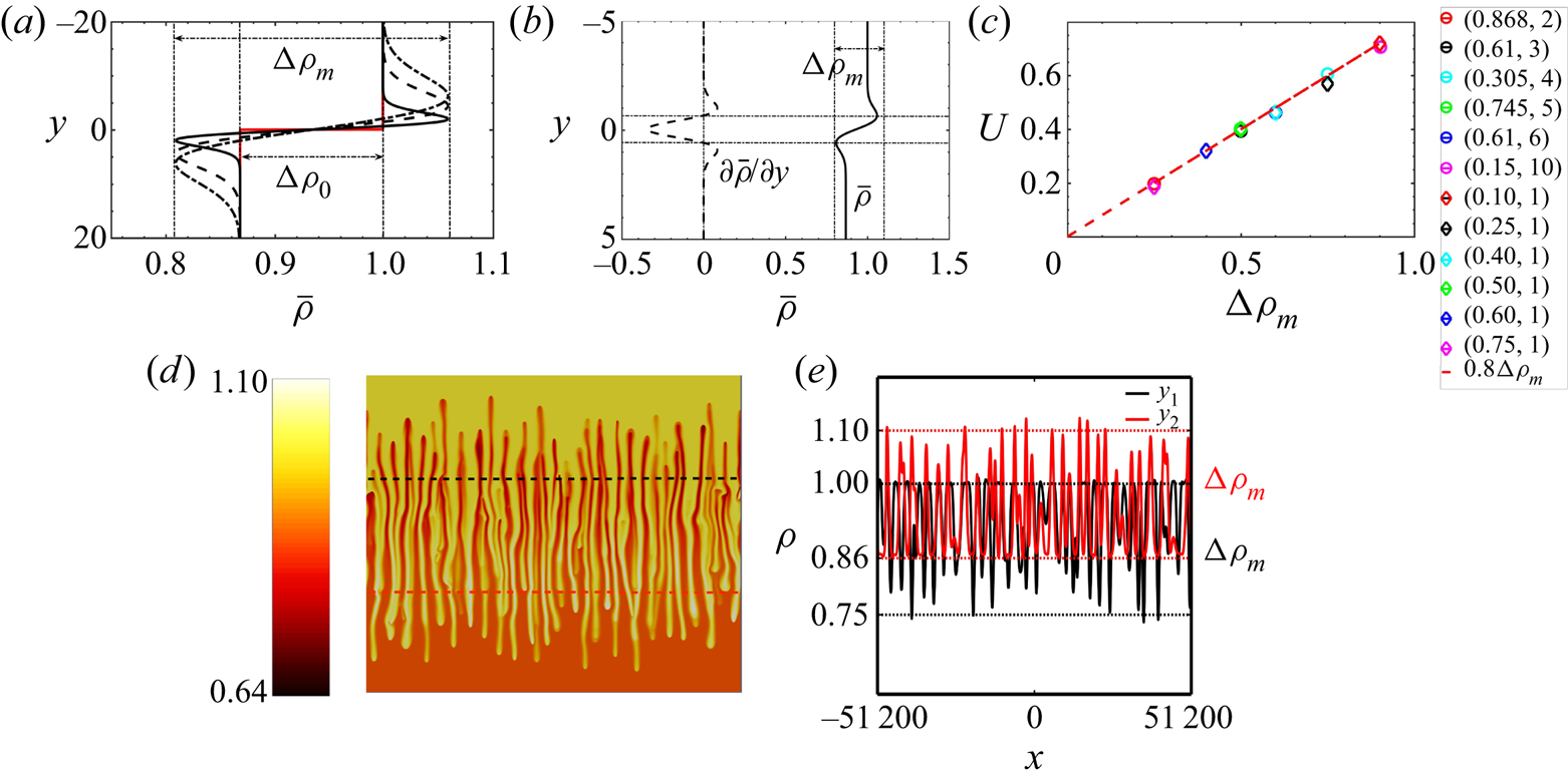
Figure 2. Characteristics of the RT–DD regime when DD modes influence the RT instability ($R<1, \delta >1$). Here, $R = 0.868, \delta = 2$. (a) Self-similar base-state density profiles at time $t=0, 1, 5, 10$. The initial profile at $t = 0$, shown in red, features the initial density jump, ${\rm \Delta} \rho _0$ whereas, as soon as $t>0$, a dynamic density jump ${\rm \Delta} \rho _m$ is triggered by the differential diffusion effects. (b) Base-state density profile $\bar {\rho }(y)$ (solid curve) and its derivative $\partial \bar {\rho }/\partial y$ (dotted curve). (c) Mixing velocity $U$ as a function of the dynamic density jump ${\rm \Delta} \rho _m$ (values of $R, \delta$ are shown for each colour point). The red line is the scaling $U = 0.8 {\rm \Delta} \rho _m$. The maximum deviation in the values of $U$ arising from the seeded initial conditions over 20 simulations is of the order $10^{-3}$. (d) Spatial distribution of the density at a given time in the nonlinear regime. The density profiles along the black and red lines denoted in (d) are shown in (e) with the amplitude of ${\rm \Delta} \rho _m, 0.25$, demarcated using dotted lines and marked as labels along the $y$ axis.

It has been shown recently both experimentally and numerically that, for $\delta >1$, this adverse dynamic density jump ${\rm \Delta} \rho _m$ (rather than ${\rm \Delta} \rho _0$) governs the velocity $U$ at which the mixing zone of the RT fingers grows (Gopalakrishnan et al. Reference Gopalakrishnan, Carballido-Landeira, Knaepen and De Wit2018). This mixing velocity $U$ is computed as the slope in the nonlinear regime of the temporal evolution of the averaged mixing length $L$ measured as the distance between the most upward and downward point of the fingered zone. As shown in figure 2(c), $U$ scales as $U = 0.8 {\rm \Delta} \rho _m$ in the zone of parameter space where $R<1$ and $\delta \geq 1$ (Gopalakrishnan et al. Reference Gopalakrishnan, Carballido-Landeira, Knaepen and De Wit2018).

This scaling of $U$ can be qualitatively understood from the spatial distribution of the density field in the nonlinear regime, as shown in figure 2(d). The variations of the density along the black and red lines passing in the middle of the upper and lower parts respectively of the fingered zone are shown in figure 2(e). The density difference between the middle of the fingers and the invaded solution ahead of it is seen to be approximately equal to ${\rm \Delta} \rho _m$ ($= 0.25$). This remains the same during the whole nonlinear regime. This shows that, even though the initial density jump is ${\rm \Delta} \rho _0$, right from the beginning, differential diffusion induces a non-monotonic density profile such that, locally, fingers experience the dynamic density difference ${\rm \Delta} \rho _m$ with the solution surrounding them. As a consequence, the mixing velocity $U$ at which the fingers move in their environment remains constant and scales as ${\rm \Delta} \rho _m$ (Gopalakrishnan et al. Reference Gopalakrishnan, Carballido-Landeira, Knaepen and De Wit2018). It is worth noting that the value of ${\rm \Delta} \rho _m$ is independent of the flow equation and can be computed analytically via (4.1) solely on the basis of the solution to the diffusive equations for the concentrations of the two solutes at hand. In the subsequent sections, we extend the scaling observed for the RT–DD regime to other regimes in the $(R, \delta )$ parameter space.

5. Scaling in the pure DD regime ($1 \leq R^{2} \leq \delta$)

The pure DD instability arises when $1 \leq R^{2} \leq \delta$ starting from an initially statically stable configuration (less dense above denser). A couple of representative base-state density profiles are shown for these cases in figure 3(a,b). The initial density profile (shown in red in figure 3a,b) is buoyantly stable (${\rm \Delta} \rho _0 = (1 - R) < 0$). However, as $\delta >1$, B diffuses faster upwards than A, which diffuses downwards. As soon as $t>0$, this induces a non-monotonic density profile with, locally, a denser zone above a less dense one across the initial interface. The amplitude of this buoyantly unstable density difference is the dynamic density jump ${\rm \Delta} \rho _m>0$, which can be computed using the values of $(R, \delta )$ via (4.1). This region with an adverse density gradient is the zone where $\partial \bar {\rho }/\partial y < 0$, as shown for the corresponding base-state profiles in figure 3(c,d).

Figure 3. Characteristics of the pure DD regime ($1 \leq R^{2} \leq \delta$). (a,b) Base-state density profiles shown at $t = 0$ (in red) and at 3 successive times for (a) $R = 1.1, \delta = 3$ and (b) $R = 1.5, \delta = 7$. (c,d) Base-state density profile $\bar {\rho }(y)$ and its derivative $\partial \bar {\rho }/\partial y$ for the parameter settings in (a,b). The dynamic density jump ${\rm \Delta} \rho _m$ that governs the rate at which the fingers grow corresponds to the difference in density between the bounds of the interval where $\partial \bar {\rho }/\partial y$ is negative.

We have numerically integrated model (2.1)–(2.4) for various values of $R$ and $\delta$ in the pure DD regime. The spatial distribution of the density field at a given time in the nonlinear regime is shown in figure 4(a,c) for two values of parameters in the $R\geq 1, \delta \geq 1$ zone. As both RT and DD instabilities have similar eigenfunctions (Trevelyan et al. Reference Trevelyan, Almarcha and De Wit2011), similar convective patterns are observed in the case of pure DD. Figure 4 shows some examples of DD fingers in the spatio-temporal distribution of the density field. From such snapshots, we can measure the mixing length as the distance between the upper and lower points of the mixing zone. Figure 5(a) shows the temporal evolution of the mixing length $L$ averaged over 20 simulations for various values of $\delta > 1$ at $R = 1.1$. We see that a linear scaling can be observed in the nonlinear regime, such as in the RT regime (Gopalakrishnan et al. Reference Gopalakrishnan, Carballido-Landeira, De Wit and Knaepen2017; De Paoli et al. Reference De Paoli, Zonta and Soldati2019). The mixing velocity $U$, computed as the slope of this linear $L(t)$ trend, is shown as a function of $\delta$ for three different values of $R$ in figure 5(b). At a fixed $R$, it increases with $\delta$, while for a given value of $\delta$ it decreases when $R$ increases. As observed in the RT–DD regime, the mixing velocity scales here linearly again with the dynamic density jump as $U = 0.8{\rm \Delta} \rho _m$ (figure 5c). To understand this scaling, we plot in figure 4(b,d) the variation of density along the black and red lines shown in figures 4(a) and 4(c) respectively. Strikingly, the adverse density jump ${\rm \Delta} \rho _m$ induced by differential diffusion effects is the density difference between the middle of the fingers and their surroundings. This explains why their averaged propagation speed quantified by $U$ scales with ${\rm \Delta} \rho _m$.

Figure 4. Spatial distribution of the density field at a given time in the nonlinear regime for (a) $R = 1.1, \delta = 3$ and (a,c) $R = 1.5, \delta = 7$. The variations of the density along the black and red lines in (a,c) are shown in (b,d). The corresponding values of ${\rm \Delta} \rho _m$ are $0.21$ and $0.25$ respectively.

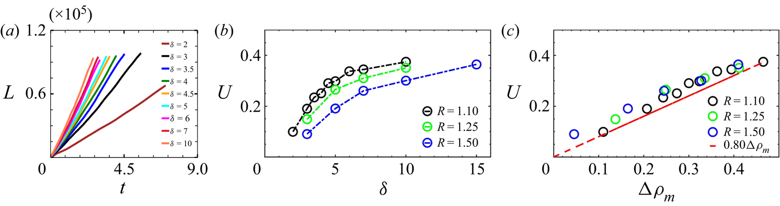
Figure 5. (a) Temporal evolution of the mixing length $L$ (averaged over 20 simulations) for $R = 1.1$ and various values of $\delta$. Mixing velocity $U$ as a function of (b) $\delta$ and (c) ${\rm \Delta} \rho _m$ at three different values of $R$. The red line in (c) is the scaling $U = 0.8{\rm \Delta} \rho _m$. The maximum deviation in the values of $U$ arising from the seeded initial conditions over 20 simulations is of the order $10^{-3}$.

In the DDD regime obtained in the parameter space for $R^{2/3} \leq \delta \leq R^{2}$, the first derivative of the base-state density profiles is strictly positive throughout the domain. Typical density profiles along with their spatial derivatives are illustrated for this regime in figure 6. Although the flows are linearly unstable, the differential diffusion effects do not lead to locally unstable zones where ${\partial \bar {\rho }}/{\partial y} < 0$ in the base-state density profiles. Hence, an adverse dynamic density jump ${\rm \Delta} \rho _m$ cannot be defined. The necessary condition for such base flows to be unstable is the presence of a point on either side of the initial interface where the second derivative of the base-state density profile is $0$, i.e. it changes its sign on either side of the initial interface (Gopalakrishnan Reference Gopalakrishnan2020). In these flows, the instability arises as stationary modes unlike in the other unstable regimes, where the growth rates can be real or complex.

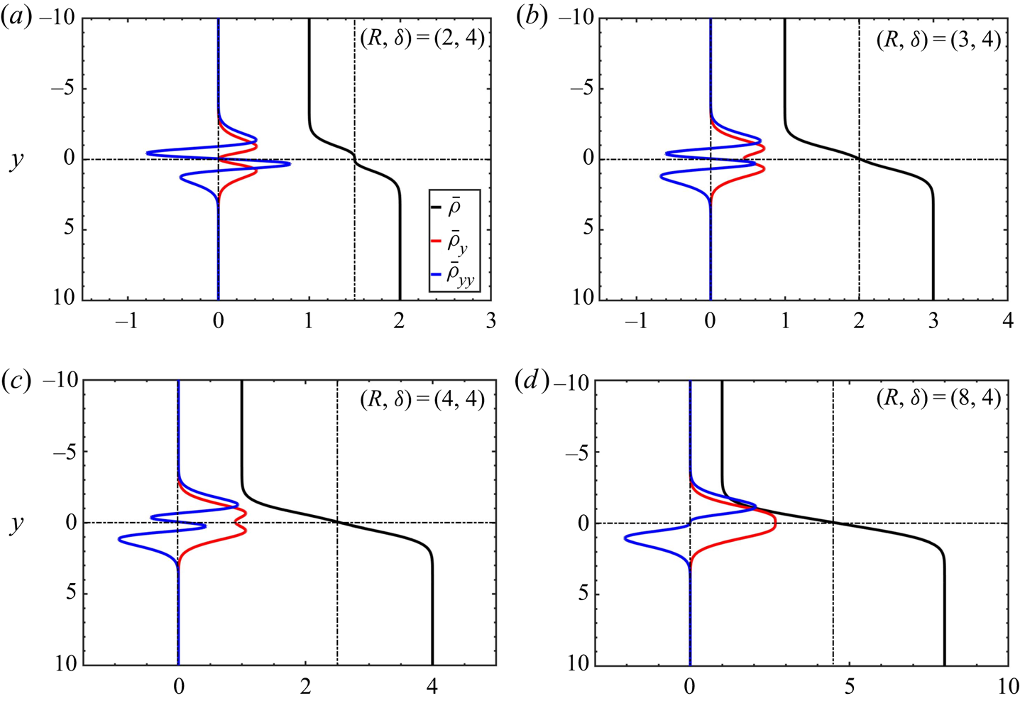
Figure 6. Typical base-state density profiles and their spatial derivatives in the DDD regime (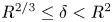$R^{2/3}\leq \delta < R^{2}$).

6. Scalings in the RT–DLC regime ($R<1, \delta <1$) and pure DLC regime ($R>1, \delta <1$)

The flow dynamics can also be influenced by DLC modes if $\delta < 1$. We analyse here the scalings of the mixing velocity $U$ in this case, both in the RT regime ($R<1$) and in the pure DLC regime ($R > 1$). When $R^{2} \leq \delta <1$, the base-state density profiles are monotonic (see figure 7a,c) with the unstable initial density difference, ${\rm \Delta} \rho _0 = 1- R$, driving the flow dynamics as observed in single-species RT flows. If $R_c \leq \delta < R^{2}$, the faster diffusion of A downwards results in a non-monotonic base-state density profile once $t > 0$. A buoyantly stable zone where $\partial \bar {\rho }/\partial y>0$ develops then across the initial interface (figure 7b,d). The amplitude of the density difference across that stable layer is the dynamic density jump ${\rm \Delta} \rho _m$ given by (4.1); ${\rm \Delta} \rho _m$ between the minimum and maximum in density has here a negative value as, locally, the density stratification is stable around the interface.

Figure 7. Base-state density profiles in RT regimes with (a) $R^{2} \leq \delta < 1$ and (b) $R_c \leq \delta <R^{2}$ where the unstable initial density difference ${\rm \Delta} \rho _0$ (shown in red) is larger than the stable stratification ${\rm \Delta} \rho _m$ that develops at $t > 0$. (c,d) The base-state density profile and its spatial derivative $\partial \bar {\rho }/\partial y$. Parameter settings: (a,c) $\delta = 0.25, R = 0.50, {\rm \Delta} \rho _m = 0, {\rm \Delta} \rho _0 = 0.50$; (b,d) $\delta = 0.25, R = 0.75, {\rm \Delta} \rho _m = -0.19, {\rm \Delta} \rho _0 = 0.25$.

We can then distinguish two different zones in the region of the parameter space $\delta <R^{2}$. They are separated by the curve $\delta = R_c$ given by $\delta = R^{n}$ (where $n \approx 6.8$) (Carballido-Landeira et al. Reference Carballido-Landeira, Trevelyan, Almarcha and De Wit2013) at which ${\rm \Delta} \rho _m={\rm \Delta} \rho _0$. First, if $R_c \leq \delta < R^{2}<1$, we have ${\rm \Delta} \rho _0 > \lvert {\rm \Delta} \rho _m\rvert$ (see figure 7b,d) and the growth of the RT mixing zone is controlled by ${\rm \Delta} \rho _0$. Once $\delta <R_c$, we have ${\rm \Delta} \rho _0<\lvert {\rm \Delta} \rho _m\rvert$ as the two extrema of the non-monotonic density profile lie outside the range of initial values of density (figure 8a). A local buoyantly stable layer separates the solutions across the initial interface while zones where locally a denser solution overlies a less dense one develop on either side of the initial interface. The typical base-state density profile and its spatial derivative is illustrated in figure 8(c). An adverse density jump ${\rm \Delta} \rho ^{\prime }_m$ can be defined across the zone where locally $\partial \bar {\rho }/\partial y<0$ on either side of the initial interface (figure 8a). Its value can be computed as

(6.1)\begin{equation} {\rm \Delta}\rho^{\prime}_m = \frac{{\rm \Delta}\rho_0 - {\rm \Delta}\rho_m}{2}, \quad \mathrm{for}\ {\rm \Delta}\rho_0 < \lvert{\rm \Delta}\rho_m\rvert, \end{equation}

with ${\rm \Delta} \rho _m$ given by (4.1).

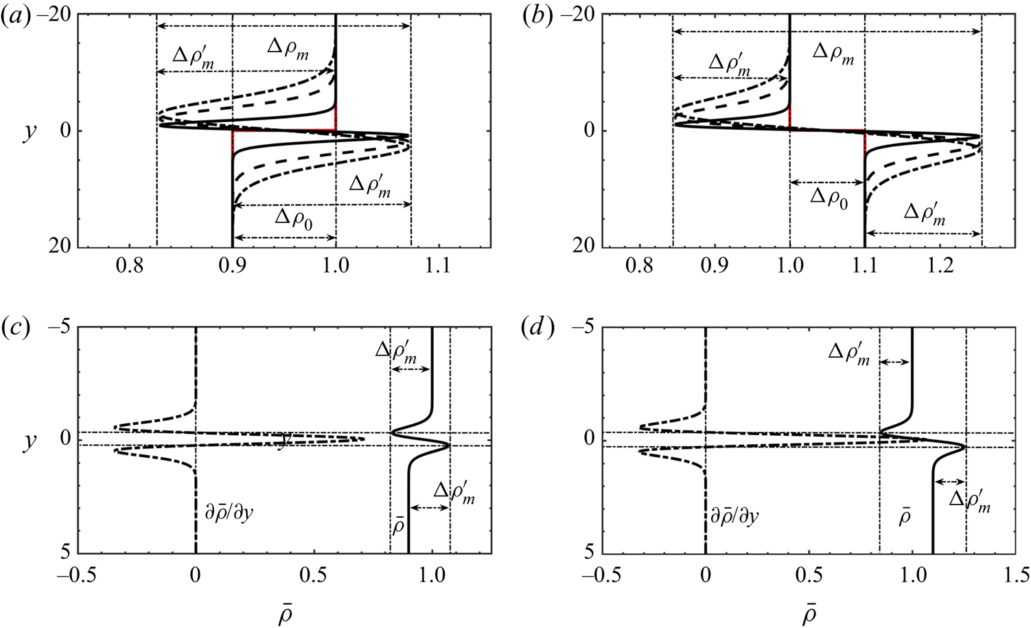
Figure 8. Base-state density profiles in (a) the RT–DLC mixed-mode regime and (b) in the pure DLC regime. (c,d) Corresponding spatial derivatives and the adverse density jump ${\rm \Delta} \rho ^{\prime }_m$. Parameter settings: (a,c) $\delta = 0.25, R = 0.90, {\rm \Delta} \rho _0 = 0.10, {\rm \Delta} \rho _m = -0.24, {\rm \Delta} \rho ^{\prime }_m = 0.17$; (b,d) $\delta = 0.25, R = 1.10, {\rm \Delta} \rho _0 = -0.10, {\rm \Delta} \rho _m = -0.41, {\rm \Delta} \rho ^{\prime }_m = 0.15$.

Similar features i.e. a non-monotonic density profile such that $\lvert {\rm \Delta} \rho _0\lvert < \lvert {\rm \Delta} \rho _m\rvert$ but with both ${\rm \Delta} \rho _0<0$ and ${\rm \Delta} \rho _m<0$ can be observed in pure DLC regimes when $R \geq 1, \delta < 1$, as shown in figure 8(b,d). As $R \geq 1$, the initial density difference ${\rm \Delta} \rho _0$ is negative, corresponding to an initially buoyantly stable configuration. In these flows, as discussed in § 3, the system destabilises due to the differential diffusion of the solutes which induces an adverse density stratification on either side of the initial interface, similar to the RT–DLC mixed-mode regime. This adverse density jump ${\rm \Delta} \rho ^{\prime }_m$, given by (6.1), is the density difference across the regions where ${\partial \bar {\rho }}/{\partial y} < 0$ as shown in figure 8(d).

The flow dynamics corresponding to the various base-state density profiles for $\delta <1$ shown in figures 7 and 8 is summarised in figure 9 giving the spatial distribution of the density field at a given time during the nonlinear regime. In the RT regime, fingers extend all across the initial position of the interface (figure 9a,b) with some fingers showing a Y-shape if $R_c \leq \delta <R^{2}$ (figure 9b). The corresponding density variation along the black and red lines is shown in figure 9(e,f). When entering the RT–DLC mixed-mode regime ($\delta <R_c$), DLC features, such as local deformation of the tip of the fingers into Y-shaped antennae, appear in addition to the RT modulation of the interface (Carballido-Landeira et al. Reference Carballido-Landeira, Trevelyan, Almarcha and De Wit2013). Figure 9(c) shows an example of such a RT–DLC mixed mode. Figure 9(d) illustrates the pure DLC dynamics characterised by a stable middle interface and convective zones developing on either side of it. The origin of the DLC mechanism can be noted in the density map where a low density zone is seen above the interface while an accumulation zone with a larger density develops below the interface. As can be seen in figure 9(h) the density difference driving the convection of the fingers is $\approx 0.16$ both above and below the interface which corresponds to the value of ${\rm \Delta} \rho ^{\prime }_m = 0.16$.

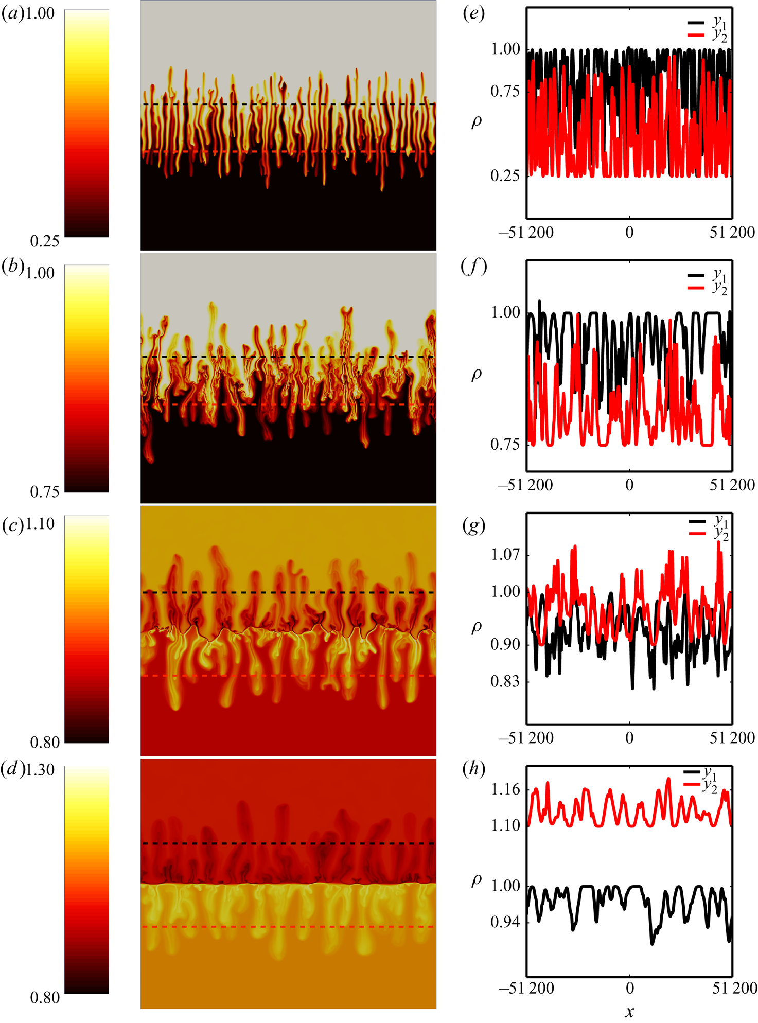
Figure 9. Spatial distribution of density fields illustrating the transition from flows dominated by (a,b) RT effects, to the (c) RT–DLC mixed-mode scenario and eventually to the (d) pure DLC mechanism. The variation of density for the corresponding flow fields along the black and red lines are shown in (e,f,g,h). Parameter settings: $\delta = 0.25$ and (a) $R = 0.25$, (b) $R = 0.75$, (c) $R = 0.90$, (d) $R = 1.1$.

Figure 10(a) plots the averaged mixing length for the RT–DLC regime. The mixing length is here still measured as the distance between the uppermost tip of fingers in the top layer to the lowest tip of the fingers in the lower layer. Figure 10(b) shows that, as $R$ increases, the mixing velocity $U$ decreases. This is due to the fact that the driving density jump decreases as well. We find numerically that the mixing velocity $U$ scales throughout the $\delta <1$ zone as $U\sim 0.8 {\rm \Delta} \rho ^{*}_{m}$ where ${\rm \Delta} \rho ^{*}_{m}$ is defined as

(6.2)\begin{gather} {\rm \Delta}\rho^{*}_{m} = {\rm \Delta}\rho_0, \quad \mathrm{for}\ \lvert{\rm \Delta}\rho_0\rvert \geq \lvert{\rm \Delta}\rho_m\rvert, \end{gather}

(6.3)\begin{gather}{\rm \Delta}\rho^{*}_{m} = 0.5 {\rm \Delta}\rho^{\prime}_{m}, \quad \mathrm{for}\ \lvert{\rm \Delta}\rho_0\rvert < \lvert{\rm \Delta}\rho_m\rvert. \end{gather}

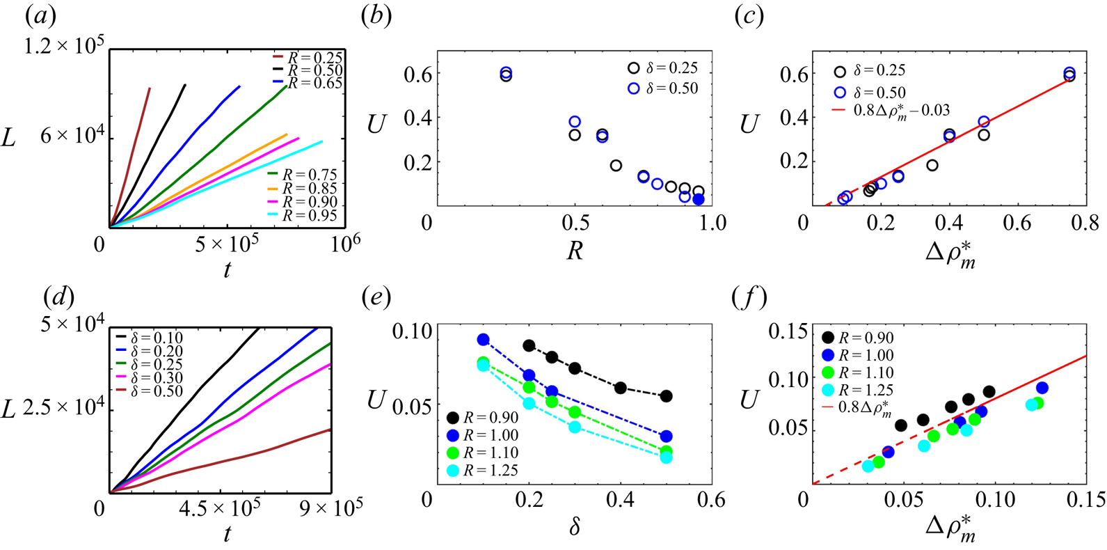
Figure 10. Temporal evolution of the mixing length $L$ (averaged over 20 simulations) for (a) variable $R$ at $\delta = 0.25$ and (d) variable $\delta$ at $R = 1.1$. Mixing velocity $U$ as a function of (b) $R$ and (e) $\delta$, and its variation with the adverse density jump ${\rm \Delta} \rho ^{*}_m$ in (c,f). Open circles indicate when ${\rm \Delta} \rho ^{*}_m$ is given by the initial density difference ${\rm \Delta} \rho _0$, and filled circles by (6.3). The maximum deviation in the values of $U$ arising from the seeded initial conditions over 20 simulations is of the order $10^{-3}$.

The scaling of the mixing velocity $U$ as a function of the adverse density jump ${\rm \Delta} \rho ^{*}_m$ is shown in figure 10(c). In figure 10(b,c,e,f), the open circles indicate that the driving force comes from the unstable initial stratification ${\rm \Delta} \rho _0$ for $\delta >R_c$ and filled circles are driven by 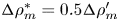${\rm \Delta} \rho ^{*}_m=0.5 {\rm \Delta} \rho ^{\prime }_m$ when $\delta <R_c$. As in the earlier flow regimes, we observe a linear relationship between $U$ and the adverse density stratification ${\rm \Delta} \rho ^{*}_m$, with $U = 0.8{\rm \Delta} \rho _0$ for $R_c \leq \delta$, and $U = 0.8{\rm \Delta} \rho ^{*}_m = 0.4{\rm \Delta} \rho ^{\prime }_{m}$ for $\delta < R_c$.

The evolution of the average mixing length in the DLC regime is shown in figure 10(d) for different values of $\delta$ and $R=1.1$. As $\delta$ decreases at a fixed value of $R$, the rate of diffusion of the solute from the upper solution to the lower one increases, which results in an increased value of the adverse density jump ${\rm \Delta} \rho ^{\prime }_m$ and thus to an increased mixing velocity $U$ (figure 10e). The mixing velocity $U$ as a function of the adverse density jump ${\rm \Delta} \rho ^{*}_m$ given by (6.2) and (6.3) is plotted in figure 10(f) where a linear scaling, $U = 0.8{\rm \Delta} \rho ^{*}_m$, can be observed. The same scaling law applies thus to both the RT–DLC mixed-mode regime and pure DLC flows, similarly to the RT–DD and DD flows. The fact that ${\rm \Delta} \rho ^{*}_m=0.5 {\rm \Delta} \rho ^{\prime }_{m}$ when 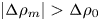$\lvert {\rm \Delta} \rho _m\rvert > {\rm \Delta} \rho _0$ is due to the fact that the density jump ${\rm \Delta} \rho ^{\prime }_{m}$ can develop only towards one side as it is bounded on the other side by a stable barrier. The extent of this stable barrier is given by ${\rm \Delta} \rho _m$ (4.1).

The transition of the adverse density jump from ${\rm \Delta} \rho _0$ to ${\rm \Delta} \rho ^{*}_m=0.5{\rm \Delta} \rho ^{\prime }_m$ in the $(R, \delta )$ plane when $\delta <1$ is summarised in figure 11(a). Figure 11(b) shows isocontours of the adverse density jump in the $\delta <1$ zone. The curve $\delta = R_c$, given by $\delta = R^{n} (n = 6.8)$ shown using a dotted line demarcates the switch from the RT regime to the RT–DLC mixed-mode and pure DLC regimes. For $\delta >R_c, {\rm \Delta} \rho _0=1-R$ is at play. When $\delta <R_c, {\rm \Delta} \rho ^{*}_m =0.5 {\rm \Delta} \rho ^{\prime }_m$ fixes the dynamics. The value of ${\rm \Delta} \rho ^{\prime }_m$ is given by (6.1) and decreases with an increase in $\delta$ at a fixed $R$. For small values of $\delta (< 0.2), {\rm \Delta} \rho ^{\prime }_m$ stays roughly constant as a function of $R$, whereas at higher values of $\delta$ it decreases slowly. Figure 11(c) summarises the scaling $U = 0.8{\rm \Delta} \rho ^{*}_m$ across values dominated by ${\rm \Delta} \rho _0$ (in black) and those ruled by ${\rm \Delta} \rho^{\prime}_{m}$ (in blue).

Figure 11. (a) Variation of ${\rm \Delta} \rho _0, {\rm \Delta} \rho _m$ and $0.5 {\rm \Delta} \rho ^{\prime }_m$ as a function of $R$ for $\delta = 0.25$, with ${\rm \Delta} \rho ^{*}_{m}$ denoted by the thick black line. The switch of ${\rm \Delta} \rho ^{*}_{m}$ from ${\rm \Delta} \rho _0$ to $0.5{\rm \Delta} \rho ^{\prime }_m$ occurs at $R = 0.915$. (b) Contours of the adverse density jump ${\rm \Delta} \rho ^{\prime }_m$ which governs the scaling of $U$ in the $(R, \delta )$ plane for $\delta <1$ illustrating the transition from the RT dominant zone for $R<R_c$ shown by the thick dotted line to the DLC-dominated regime when $R>R_c$. In the RT zone, the adverse density jump is ${\rm \Delta} \rho _0=1-R$ and the scaling of the mixing velocity is $U=0.8 {\rm \Delta} \rho _0$. In the RT–DLC mixed-mode and pure DLC regimes, we have $U=0.8 {\rm \Delta} \rho ^{*}_m = 0.5{\rm \Delta} \rho ^{\prime }_m$. This is shown in panel (c), where the velocity $U$ is shown as a function of ${\rm \Delta} \rho ^{*}_m$ for $\delta < 1$ ($\delta = [0.10, 0.20, 0.25, 0.30, 0.50]$), with $R$ ranging from $0.25$ to $1.25$.

7. Summary and discussion

Different buoyantly unstable scenarios can be obtained depending on the values of the two non-dimensional parameters $R$ and $\delta$ that govern the flow dynamics. The miscible interface is subject to a RT instability when $R < 1$. The single-species RT instability occurs when $\delta = 1$. In that case, the density is decreasing monotonically along the gravity field and $U$ scales as $0.8{\rm \Delta} \rho _0$ where ${\rm \Delta} \rho _0 = 1 - R$ is the initial density difference.

In the case of two-species RT–DD stratification, if the species in the lower solution diffuses faster ($\delta > 1$), the density profiles have a non-monotonic spatial dependence with a maximum in density above the interface and a minimum in density in the lower layer as soon as $t > 0$. The adverse density jump ${\rm \Delta} \rho _m$ between these extrema is larger than the initial density difference ${\rm \Delta} \rho _0$, and can be computed analytically from the diffusive base-state concentration profiles using the values of $R$ and $\delta$ via (4.1). The mixing velocities computed in the corresponding nonlinear RT regime are found to scale linearly as $U = 0.8{\rm \Delta} \rho _m$. This is due to the fact that the density difference experienced by the fingers with the solution ahead of them during their nonlinear evolution is approximately ${\rm \Delta} \rho _m$. For $\delta >1$ and a buoyantly stable initial configuration ($R \geq 1$) such that ${\rm \Delta} \rho _0<0$, DD effects result in an adverse density difference ${\rm \Delta} \rho _m>0$ across the miscible interface due to the faster upwards diffusion of the species from the lower layer. In the nonlinear regime, the mixing velocity $U$ is found to scale linearly with this adverse density difference as $U = 0.8{\rm \Delta} \rho _m$. The footprint of ${\rm \Delta} \rho _m$ can be observed in the nonlinear regime from the spatial distribution of the density fields with the density difference between the fingers and their surroundings being ${\rm \Delta} \rho _m$.

If $\delta <1$, other scenarios are encountered. If $R^{2} \leq \delta <1$, the RT density profiles are monotonically decreasing downwards and the flow dynamics is governed by the initial density difference ${\rm \Delta} \rho _0$ with $U = 0.8{\rm \Delta} \rho _0$. For $R_c \leq \delta < R^{2}$, the non-monotonic density profiles feature a locally stable stratification across the initial interface where ${\rm \Delta} \rho _m<0$. In this regime, the initial density difference ${\rm \Delta} \rho _0$ still drives the convective mixing globally and $U = 0.8{\rm \Delta} \rho _0$ even though the influence of differential diffusion can be seen at the tips of some fingers. For $\delta \leq R_c < 1$, when the absolute value of the locally stable stratification ${\rm \Delta} \rho _m\,(<0)$ exceeds the initial density difference ${\rm \Delta} \rho _0>0$, an adverse density difference ${\rm \Delta} \rho ^{\prime }_m$ given by (6.1) can be observed on either side of the interface. In this RT–DLC mixed-mode regime, where DLC effects strongly influence the RT flow dynamics, ‘Y-shaped antenna-like’ structures can be observed developing around the interface. Similar features in the density profiles can also be observed in a buoyantly stable stratification $R>1$ with $\delta < 1$ where only pure DLC mechanisms are present. The mixing velocities in these regimes decrease with increasing $R$ and $\delta$, and are found to scale linearly as $U = 0.8{\rm \Delta} \rho ^{*}_m = 0.4{\rm \Delta} \rho ^{\prime }_{m}$. For the RT–DLC mixed-mode and pure DLC scenarios, the instability develops separately above and below the interface, with ${\rm \Delta} \rho ^{*}_m$ driving the convection that develops independently on either side of the mixing zone.

In all the scenarios discussed in this study, the most striking observation is that the driving force for the mixing velocity of the fingers is always the density difference experienced by the fingers with their surroundings. This density difference, although computed analytically from the base-state diffusive density profiles, persists in the nonlinear regime, and imprints therefore its influence on the mixing velocity $U$. This is illustrated in figure 12 which shows the distribution of the density field within our computational domain at a given time in the nonlinear regime for the different scenarios discussed in the present study in the $(R, \delta )$ parameter space. For (a) RT and (e) DD instabilities, the distribution of the density field shows that the density difference experienced by the fingers with their surroundings on either side of the initial interface is ${\rm \Delta} \rho _m$. When $R_c \leq \delta < 1$ i.e. for RT-dominated flows (b,c), the initial density difference ${\rm \Delta} \rho _0 = 1 - R$ drives the convective mixing. For the flows corresponding to the (d) RT–DLC mixed-mode regime and the (f) pure DLC, ${\rm \Delta} \rho ^{*}_m = 0.5{\rm \Delta} \rho ^{\prime }_m$ is the density difference which governs the evolution of the mixing length.

Figure 12. Distribution of the values of the density field within our computational domain at a given time in the nonlinear regime for the various scenarios discussed in the present study. The density difference ${\rm \Delta} \rho$ driving the evolution of the mixing length on either side of the initial interface $y = 0$ is: (a) RT–DD: $R < 1, \delta \geq 1, {\rm \Delta} \rho = {\rm \Delta} \rho _m$; (b) RT: $R < 1, R^{2} < \delta < 1, {\rm \Delta} \rho = {\rm \Delta} \rho _0 = 1 - R$; (c) RT: $R < 1, R_c < \delta < R^{2}, {\rm \Delta} \rho = {\rm \Delta} \rho _0$; (d) RT–DLC: $R < 1, \delta < R_c, {\rm \Delta} \rho = 0.5{\rm \Delta} \rho ^{\prime }_m$; (e) DD: 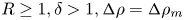$R \geq 1, \delta > 1, {\rm \Delta} \rho = {\rm \Delta} \rho _m$; (f) DLC: 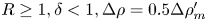$R \geq 1, \delta < 1, {\rm \Delta} \rho = 0.5{\rm \Delta} \rho ^{\prime }_m$. Parameter settings: (a) $R = 0.868, \delta = 2$, (b) 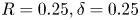$R = 0.25, \delta = 0.25$, (c) 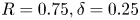$R = 0.75, \delta = 0.25$, (d) 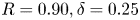$R = 0.90, \delta = 0.25$, (e) 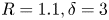$R = 1.1, \delta = 3$, (f) 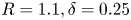$R = 1.1, \delta = 0.25$.

A summary of the different scalings can be seen in the various shaded zones of figure 1 with the shaded blue region corresponding to $U=0.8{\rm \Delta} \rho _m$ (RT–DD regime and pure DD modes), the green region to $U=0.8{\rm \Delta} \rho _0$ (RT dominant modes at $\delta <1$) and the pink region to $U=0.8{\rm \Delta} \rho ^{*}_m = 0.4{\rm \Delta} \rho ^{\prime }_m$ (RT–DLC mixed mode and pure DLC modes).

The fact that the fingers extend vertically at a speed proportional to the largest adverse density jump may sound intuitive at first sight. It certainly is intuitive in the case of the pure one-species RT instability where the density difference ${\rm \Delta} \rho _0$ between the upper solution of A and the lower layer of pure solvent controls the dynamics. The situation is less intuitive for two-species stratification. If you consider solutions of salt and sugar, different velocities will be observed even if starting from the same ${\rm \Delta} \rho _0$ because salt diffuses approximately 3 times faster than sugar. If the denser layer of salt overlies a less dense solution of sucrose, we have $\delta =1/3$. Then, even if starting with the same ${\rm \Delta} \rho _0$, the RT instability will be influenced by DLC effects for $R_c \leq R<1$ in the RT–DLC zone. The mixing velocity will then scale linearly with ${\rm \Delta} \rho ^{*}_m$. If, in contrast, we start from a denser layer of sugar above a less dense solution of salt then $\delta =3$ and ${\rm \Delta} \rho _m$ becomes the relevant density jump. Table 2 from the supplemental information of Gopalakrishnan et al. (Reference Gopalakrishnan, Carballido-Landeira, Knaepen and De Wit2018) lists a series of values of ${\rm \Delta} \rho _0$ and ${\rm \Delta} \rho _m$ that can guide experimentalists in new experiments devoted to test our predictions.

Our results also allow us to understand why, in the experiments of Pringle and Glass (Pringle & Glass Reference Pringle and Glass2002) on the DD instability, the velocity with which the fingers advance vertically remains almost the same even when concentrations are varied at a fixed $\delta$ (see figure 10 in their article). This can be explained by the fact that the change in concentrations was done by maintaining $R$ at a constant value as they were changing the values of initial concentrations $A_0$ and $B_0$ in the same proportion (see table $1$ of their manuscript).